Sensitivity study of generalised frequency response functions

This is a repository copy of

Sensitivity study of generalised frequency response functions

.

White Rose Research Online URL for this paper:

http://eprints.whiterose.ac.uk/74626/

Monograph:

Li, L.M. and Billings, S.A. (2008) Sensitivity study of generalised frequency response

functions. Research Report. ACSE Research Report no. 969 . Automatic Control and

Systems Engineering, University of Sheffield

[email protected] https://eprints.whiterose.ac.uk/ Reuse

Unless indicated otherwise, fulltext items are protected by copyright with all rights reserved. The copyright exception in section 29 of the Copyright, Designs and Patents Act 1988 allows the making of a single copy solely for the purpose of non-commercial research or private study within the limits of fair dealing. The publisher or other rights-holder may allow further reproduction and re-use of this version - refer to the White Rose Research Online record for this item. Where records identify the publisher as the copyright holder, users can verify any specific terms of use on the publisher’s website.

Takedown

If you consider content in White Rose Research Online to be in breach of UK law, please notify us by

Sensitivity Study of Generalised

Frequency Response Functions

L.M.Li

and S.A.Billings

Department of Automatic Control

and Systems Engineering,

University of Sheffield, Sheffield

Post Box 600 S1 3JD

UK

1

Sensitivity Study of Generalised Frequency Response

Functions

L.M.Li* and S.A.Billings

Department of Automatic Control and Systems Engineering

University of Sheffield, Mappin Street, Sheffield S1 3JD

*[email protected]

Abstract: The dependence and independence of input signal amplitudes for

Generalised Frequency Response Functions(GFRF’s) are discussed based on parametric modelling.

Keywords: weakly nonlinear systems ,GFRF, NARX

1. Introduction

For time-invariant linear systems, the frequency response function has proved to be one of the most important tools in the design, analysis and control of linear systems. The frequency response is inherent, invariant and totally independent of the input signals, and therefore it is always desirable as a linear description of the underlying system.

However, most physical systems are nonlinear to some extent. When the nonlinear nature of a system has to be taken into account, the classical linear frequency response description is no longer sufficient and Generalised Frequency Response Functions (GFRF’s) are introduced for the class of nonlinear systems that has a valid Volterra series representation, also called weakly nonlinear systems. As in the linear case, the GFRF’s can reveal important inherent insights into the operation of complex nonlinear behaviours that can be related back to the time domain properties and model terms. Unlike the linear case where the frequency response function is always invariant and independent of the input signals, in some situations the GFRF’s will no longer always remain invariant for all input signals in the frame of weak nonlinearity.

In this paper the sensitivity to input amplitude of the GFRF’s is investigated and the modelling of systems which fall outside the standard GFRF invariant range is analysed.

2. Volterra Series Modelling and Generalised Frequency Response Functions

system, with u(t)andy(t)the input and output respectively, the Volterra series can be expressed as

∑

y (1.a)

where y t_n( ) is the ‘n-th order output’ of the system

y t_n h_{n n} u t _i d _i

i n ( )= ⋅⋅⋅ ( , , )⋅⋅⋅ ( − ) −∞ ∞ −∞ ∞ =

∫

∫

∏

1

n>0 (1.b)

h_n( , ,τ₁⋅⋅⋅τ_n) is called the ‘nth-order Kernel’ or ‘nth-order impulse response function’. If n=1, this reduces to the familiar linear convolution integral.

The discrete time domain counterpart of the continuous time domain SISO Volterra expression (1) is

∑

y (2.a)

where

∑ ∑

∏

n k h u k

y

1

1, , ) ( )

( )

( L τ τ τ n>0,k∈Ζ (2.b)

Systems that can be adequately represented by a Volterra series are called weakly or mildly nonlinear systems. In practical problems only a finite Volterra series can be used, on the assumption that the contribution of the higher order kernels falls off rapidly. This is called the truncated Volterra series.

For discrete-time systems the truncated, discrete-time Volterra series is given as

∏

∑

∑

∑

n k h u k

y n 1 1 0 1 0 ) ( ) , , ( ) ( 1 τ τ τ τ τ

L n>0,k∈Ζ (3)

A discrete time Volterra series is also called a NX (Nonlinear model with eXogenous inputs) model.

The multi-dimensional Fourier transform of hn(⋅)yields the ‘nth-order frequency response function’ or the Generalised Frequency Response Function (GFRF):

n n n n n n

n h j d d

H ω ⋅ ⋅⋅ω =

∫ ∫

∞ −

∞ ∞

− 1 1 1 1

1, , ) ( , , )exp( ( ))

( (4)

Once the GFRF’s are available, the steady-state response of the nonlinear system, excited by an harmonic signal at frequencyω, is given by

L L + − + + − + + = } ) , , ( Re{ ) 2 ( 6 } ) , , ( Re{ ) 2 ( 2 )} , ( Re{ ) 2 ( 2 } ) , ( Re{ ) 2 ( 2 )} ( Re{ ) ( 3 3 3 3 3 2 2 2 2 2 1 t j t j t j e H E e H E H E e H E H E t y ω ω ω ω ω ω ω ω ω ω ω ω ω ω (5)

where E is the amplitude of the input signal.

3

for characterising nonlinear phenomena. The inherent features of the underlying nonlinear systems can be studied using the GFRF’s(Bedrosian and Rice, 1971; Bussgang, et. al., 1974), and this provides an analogous theory to linear frequency response analysis, which is so important for linear systems. Many nonlinear phenomena have been analysed and interpreted in terms of the GFRF’s, including gain compression, intermodulation effects, harmonics and desensitisation (Billings and Tsang, 1989).

In practice, the GFRF’s can be estimated using non-parametric or parametric methods. The parametric method involves mapping a nonlinear differential equation (Billings and Peyton Jones, 1990) or mapping a nonlinear difference equation (Peyton Jones and Billings, 1989) into the frequency domain using an extension of the probing method.

The GFRF’s derived from the parametric continuous time or discrete time models are only related to the coefficients of the models, and are independent of the input signals, therefore they are generally considered as an invariant property of the underlying system. However, the field covered by the parametric GFRF’s does not necessarily totally overlap with the field that has a convergent Volterra series representation. The frequency response functions that fall outside the parametric GFRF’s capacity become variant, being dependent on the input amplitudes.

3. Sensitivity Issues

Consider a second order dynamic system with quadratic nonlinearity as

y+ y+y+ y2 =u

28 . 0 04

. 0 01 .

0 && & (6)

) sin( whereu =E ωt

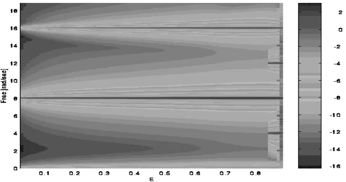
The Response Spectrum Map(RSM), introduced by Billings and Boaghe(2001), for system (6) which is excited at the frequency ω=8rad/sec, is plotted in Figure 1.

Figure 1. Response Spectrum Map for the continuous time system (6)

representation. For E∈[0.85,0.9] it can be seen that ½ order subharmonics occur, and these develop to ¼ order subharmonics forE∈[0.9,0.92]. When E∈[0.92,0.94]the response becomes chaotic, and finally for E >0.94the system becomes unstable. It is well known that Volterra series can not model systems that exhibit severe nonlinear phenomena such as subharmonics and chaos, therefore only the amplitude range

) 85 . 0 , 0 [

∈

E where a valid Volterra representation is available will be investigated in this study.

As explained in Section 2 the time domain Volterra series representation can be mapped into the frequency domain to obtain the GFRF’s, which in this example can be expressed using the coefficients of equation (6) as

1 04 . 0 ) ( 01 . 0 ) (

2 1

+ +

=

ω ω

ω

j j

E

H (7.a)

1 ) (

04 . 0 )] (

[ 01 . 0

) ( ) ( 28 . 0 )

, (

2 1 2

2 1

2 1 1 1 2

1 2

+ + +

+ =

ω ω ω

ω

ω ω ω

ω

j j

H H

H (7.b)

M M

Ideally the GFRF’s in equation (7) for the system (6) will cover the whole amplitude range E∈[0,0.85) where the system shows a Volterra series existence. But studies show that in most systems the GFRF’s obtained from the underlying system model can only cover part, and in some cases a quite small part, of the whole amplitude range.

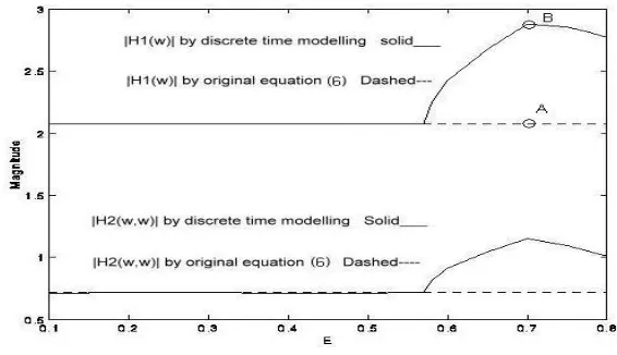
The GFRF’s can be derived from either continuous time or discrete time models. The discrete time modelling, namely NARX modelling, is capable of capturing the frequency domain features of weakly nonlinear systems in almost every circumstance, therefore the dependence or sensitivity of the original underlying system to the input amplitude can be illustrated by constructing the valid GFRF’s from discrete time modelling and comparing the results with those from the original system, against a varying amplitudeE, as shown in Figure 2. The GFRF’s from the original system (6), which are constants, are shown in Figure 2 as dashed lines. Only the first two orders of GFRF’s are shown, these are the two most significant frequency response functions associated with the dominant frequency components in the response.

5

Figure 2 shows two lines in each comparison. The solid line represents the valid GFRF’s from discrete time modelling while the dashed line represents the ideal original GFRF’s from (6). It can be seen from Figure 2 that for the lower amplitude range, both H1(⋅)and H2(⋅)from the discrete time modelling overlap with the results

from the original continuous time model (6), indicating that the GFRF’s from model (6) are valid and invariant over this lower amplitude range. The turning point occurs at E=0.58 where H₁(⋅)and H₂(⋅)from the discrete time modelling depart from the original H₁(⋅)and H₂(⋅), indicating that from this point on, the original H₁(⋅)and

) (

2 ⋅

H from equation (6) will no longer be able to provide a good frequency domain interpretation.

4. Modelling in the time and frequency domain

In section 3 it has been shown that the GFRF’s from the original system model are not always independent of the level of excitation. In this section a specific case where the operating input amplitude falls outside the independence zone will be explored for further discussion.

The input-response data was collected by simulating the system (6) at rad/sec

8

=

ω and E=0.7 using a fourth order Runge-Kutta algorithm at a sampling frequency fs =1/80with zero initial conditions. From Figure 2 the amplitude value

E=0.7 is clearly within the input dependent zone.

First, by setting both the input-output lags as 2 and using the OLS algorithm(Billings

et. al, 1989) to choose the first 4 most significant terms, a NARX model can be obtained as

) 1 ( 015252 .

0 ) 1 ( 0042572 .

0 ) 2 ( 95105 . 0 ) 1 ( 9358 . 1 )

( = − − − − 2 − + −

k u k

y k

y k

y k

y (8)

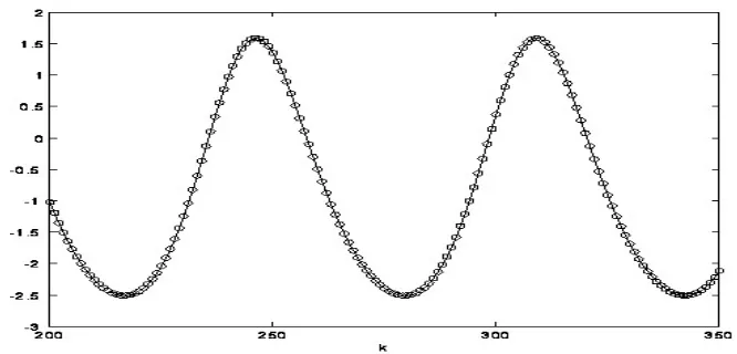
The Model Predicted Output(MPO) is shown in Figure 3, which fits perfectly to the real response.

Figure 3. MPO by estimated model (8): Solid –real response; circle--MPO

Figure 4. Comparison of H₁(ω)from (6) and (8)

By using the recursive approach in Li and Billings(2001), an estimated continuous time model can be easily reconstructed from (8) in the frequency domain, as in equation (9), which is an unbiased estimation of the original model (6).

u y

y y

y 0.04015048 0.2802 1.003471 01000125

.

0 _&&+ _&+ + 2 =

(9)

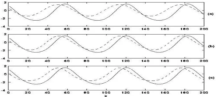
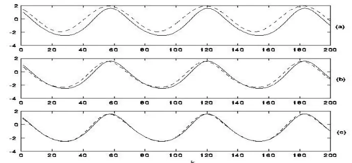
When the GFRF’s from either model (6) or model (9) are employed to analyse the response using (5), the synthesized response, however, will not converge to the real value even with up to 5th order GFRF’s considered. This is shown in Figure 5. This means that the GFRF’s are not completely valid in the frequency domain.

Figure 5. (a) First order output response, (b) up to the third order response and (c) up to 5th order response: Solid -- original output; Dashed-- synthesized output by GFRF’s

from model(8)

7

Equation (10) can be mapped into the frequency domain to generate the GFRF’s. The first order GFRF’s corresponds to the point B on the solid line in the sensitivity curve in Figure 2. Computation of the response using (5) is shown in Figure 6.

Figure 6. (a) First order output response, (b) up to the second order response and (c) up to third order response: Solid -- original output; Dashed-- synthesized output by

GFRF’s from model(10)

It can be seen from Figure 6 that the first 3 orders of GFRF’s from (10) have already succeeded in providing a satisfactory analysis of the response in the frequency domain.

In summary, two discrete time modelling tests were carried out based on the same input-response data. The only difference is the number of model terms forced into the final models. However, this difference generates a fundamental difference in terms of frequency domain interpretations. The first discrete time model will generate ‘GFRF’s’ that have no real frequency domain explanation but can be used to trace back to the time domain expression to accomplish a physical interpretation of the underlying system. To this end this procedure can be regarded as time domain physical modelling. The second model will generate real GFRF’s that are capable of performing a frequency domain analysis at the cost of more complicated time domain expression, the loss of physical interpretation and local validity. This can therefore be regarded purely as frequency domain modelling.

5. Conclusions

The Volterra series has been applied widely in representing weakly nonlinear systems. The frequency domain transform of the Volterra kernels, known as the GFRF’s, has served as an important tool in the analysis and control of nonlinear systems. Ideally the GFRF’s should be independent of the input signals, representing the invariant and inherent properties of the underlying system. However, this may not always be the case, and this study has shown that in some circumstances the invariance of the GFRF’s will vanish as the amplitude of excitation increases above a certain level.

Due to this input amplitude sensitivity or dependency, in general invariant GFRF’s may only be possible over a lower range, some times quite a limited range, of input amplitudes. Outside this amplitude range, it is generally not possible to build a model that provides locally invariant GFRF’s.

This study showed that a simple discrete time model, normally parsimonious, can preserve all the time and frequency domain features of the underlying system, but can fail in terms of practical frequency domain analysis. A different discrete time model, generally non-parsimonious, can however be estimated to accommodate the demand of frequency domain analysis. The GFRF’s from the latter model, however, have restricted ability and applicability, due to the input amplitude dependency.

An important time domain identification objective is to be able to build parsimonious models. This study suggests that the seemly redundant terms from the viewpoint of time domain representation may play a vital part in the system frequency domain representation.

Acknowledgement: SAB and LML gratefully acknowledge that this research was

supported by the UK Engineering and Physical Sciences Research Council.

References:

Bedrosian, E. and Rice, S.O., 1971, The output properties of Volterra systems (nonlinear systems with memory) driven by harmonic and Gaussian inputs, Proc. IEEE, Vol 59, pp.1688-1707.

Billings, S.A. and Boaghe, O.M., 2001,The response spectrum map, a frequency domain equivalent to the bifurcation diagram, Int. J. of Bifurcation and Chaos, Vol.11, No.7, pp.1961-1975.

Billings, S.A. and Peyton Jones, J. C., 1990, Mapping non-linear integro-differential equations into the frequency domain, Int. J. Control, Vol. 52, No. 4, pp.863-879.

Billings, S.A and Tsang, K.M., 1989, Spectral analysis for nonlinear systems, Part II—interpretation of nonlinear frequency response functions, J. Mech Systems and Signal Processing, Vol. 3, No. 4, pp341-359.

Bussgang, J.J., Ehrman, L. and Graham, J.W.,1974, Analysis of nonlinear systems with multiple inputs, Proc. IEEE, Vol 62, No. 8, pp.1088-1119.

Li, L.M. and Billings, S.A., 2001, Continuous time non-linear system identification in the frequency domain, Int J Control, 74 (10), pp. 1052-1061.

Peyton Jones, J. C. and Billings, S.A, 1989, “A Recursive algorithm for computing the frequency response of a class of non-linear difference equation models,” Int. J. Control, Vol.50, No.5, pp.1925-1940, 1989.