This is a repository copy of
Physical characteristics of subglacial tills
.
White Rose Research Online URL for this paper:
http://eprints.whiterose.ac.uk/4743/
Article:
Clarke, B.G., Hughes, D.B. and Hashemi, S. (2008) Physical characteristics of subglacial
tills. Géotechniques, 58 (1). pp. 67-76. ISSN 1751-7656
https://doi.org/10.1680/geot.2008.58.1.67
eprints@whiterose.ac.uk https://eprints.whiterose.ac.uk/ Reuse
See Attached
Takedown
If you consider content in White Rose Research Online to be in breach of UK law, please notify us by
Clarke, B. G., Hughes, D. B. & Hashemi, S. (2008). Ge´otechnique58, No. 1, 67–76 [doi: 10.1680/geot.2008.58.1.67]
67
Physical characteristics of subglacial tills
B. G . C L A R K E*, D. B. H U G H E S † a n d S . H A S H E M I †
A regional database of the physical properties of glacial tills has been interrogated to produce characteristic de-sign values and baseline construction values. Glacioterres-trial glacial till, one of the most distributed deposits in the world, is typically a heterogeneous mixture of clays, silts, sands, gravels and cobbles, which can contain rem-nants of earlier till including glaciolacustrine and fluvio-glacial deposits that have been gravitationally compacted and sheared. This results in a complex deposit, which is spatially variable both in composition and fabric to the extent that the selection of design profiles is challenging. A study of the intrinsic properties of the tills in the North East of England together with a statistical analysis has led to the identification of two distinctly different, heavily overconsolidated tills that have profiles of strength, water content and density that lead to charac-teristic values based on the regional database and base-line values based on the local database that provide a
priori knowledge for future investigations. This a priori
knowledge has been used to determine the characteristic and baseline values for a new dataset from the region after demonstrating that the data fit with the regional database.
KEYWORDS: geology; glacial soils; site investigation; design
On a interroge´ une base de donne´es re´gionale des pro-prie´te´s physiques des moraines argileuses pour produire des valeurs de calcul caracte´ristiques et des valeurs de construction de re´fe´rence. Les moraines argileuses glacio-terrestres , un des de´poˆts les plus re´pandus dans le monde entier, se composent ge´ne´ralement d’un me´lange he´te´roge`ne d’argiles, de limon, de sables, de graviers et de galets, pouvant contenir des restes de moraines pre´-ce´dentes, y compris des de´poˆts lacustres glaciaires et fluviaux compacte´s et cisaille´s par gravitation. On obtient ainsi des de´poˆts complexes, a` composition et structure spatiale variables, au point de rendre difficile la se´lection de profils caracte´ristiques. Une e´tude des proprie´te´s in-trinse`ques des moraines du nord-est de l’Angleterre, ainsi qu’une analyse statistique, ont permis d’identifier deux moraines particulie`rement diffe´rentes et fortement sur-consolide´es, pre´sentant des profils de re´sistance, teneur en eau et densite´, permettant d’obtenir des valeurs car-acte´ristiques fonde´es sur la base de donne´es re´gionale et des valeurs de re´fe´rence de´coulant de la base de donne´es locale, constituant des connaissances a` priori pour des examens futurs. On a utilise´ ces connaissances a` priori pour de´terminer les valeurs caracte´ristiques et de re´fe´r-ence pour un nouvel ensemble de donne´es pour la re´gion, apre`s avoir de´montre´ que les donne´es sont conformes a` la base de donne´es re´gionale.
INTRODUCTION
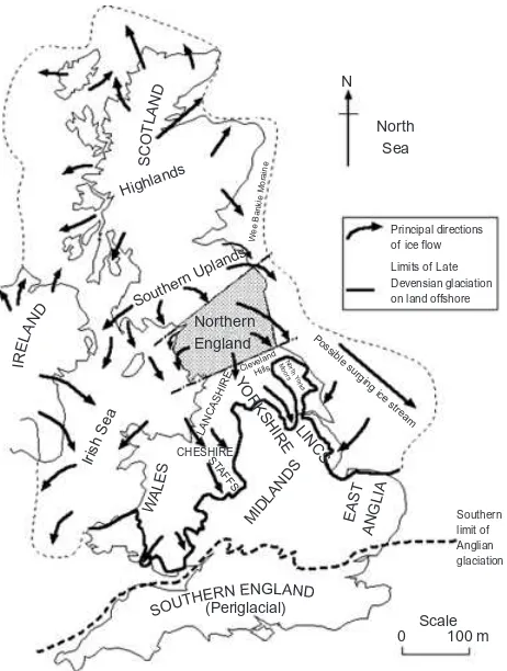
Over 60% of the British Isles was covered by an ice sheet at
some time (Hughes et al., 1998), resulting in extensive
glacioterrestrial and glaciofluvial deposits (Fig. 1) that are typical of some of the most widely distributed deposits in the world. The most common of these deposits, the glacio-terrestrial deposits, were either formed subglacially as lodge-ment till or deformation till or deposited from within the ice of a retreating glacier in the form of melt-out till or flow till. The lodgement and deformation tills are typically het-erogeneous mixtures of clays, silts, sands, gravels and cob-bles that have been gravitationally compacted and sheared under several different temperature profiles. Melt-out tills are subglacial, supraglacial or englacial deposits that can be similar in composition to other subglacial tills but can also include extensive lenses of clays, sands and gravels.
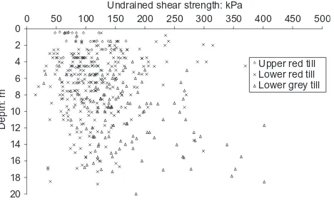
Quality sampling is usually restricted to clay-matrix-dominant till that is free of cobbles. Any gravel present, which is usual, may affect the sampling, and lead to a wide range of test results for a given property, making it difficult to select design parameters unless there is a clear set of rules to take into account the natural variability and the impact the fabric and composition have upon the derived parameters. For example, Fig. 2 shows a profile of undrained
Manuscript received 18 September 2006; revised manuscript accepted 16 August 2007.
Discussion on this paper closes on 1 July 2008, for further details see p. ii.
* School of Civil Engineering and Geosciences, University of Newcastle-upon-Tyne, UK.
† Formerly University of Newcastle-upon-Tyne, UK
Irish Sea
N
North Sea
Principal directions of ice flow Limits of Late Devensian glaciation on land offshore
Southern limit of Anglian glaciation
Scale
0 100 m
Possible
surging
ice stream
Wee Bankie
Mor aine
ClevelandHills
Nor th Yor
ks Moor
s
Highlands
Northern England
EAST ANGLIA MIDLANDS
ST AFFS LANCASHIRE CHESHIRE
LINCS
S
CO
TL AN
D
Souther n Uplands
YORKSHIRE
[image:2.595.306.537.424.730.2](Periglacial)
shear strength of clay-matrix-dominant tills from a site in the North East of England. This paper uses an extensive database of physical characteristics of tills from the North East of England to demonstrate the difficulty, and develops a framework to identify the design values of subglacial tills. The data are taken from routine ground investigations that were carried out according to the British Standard current at the time of the investigation. The framework is based on a statistical method suggested by Eurocode 7 (2004) to provide characteristic values for design, and applies the same method to assess baseline values for construction.
FORMATION OF TILL
Tills are formed either by gravitational compaction and shearing (lodgement and deformation tills), which takes place as the ice advances, or by gravitational compaction (melt-out and flow tills), which takes place as the ice either advances or retreats. Glacial velocities exceeding 50–100 m/ year would be sufficient to erode an existing till (Boulton & Paul, 1976). It is likely that tills have been reworked and redeposited a number of times during successive periods of glaciation, such that many of the deposits identified today include remnants of previous glaciations laid down during the last glacial period. Thus deformation till may contain remnants of earlier till including glaciolacustrine and fluvio-glacial deposits, that is, intraformational sands, gravels and laminated clays that have been deposited in subglacial or englacial meltwater channels and lakes (Eyles & Sladen, 1981). As the ice advances, the subglacial till is increasingly
mixed and deformed, leading to lodgement till (Hughes et
al., 1998). There is anecdotal evidence that the fines content
of tills increases towards the coast in the principal direction of the ice flow (see Fig. 1). A number of pore pressure regimes could have existed, depending on whether the
glacier was formed of temperate or cold ice (Boultonet al.,
1976), on the permeability of the underlying rock and the temperature profile through the till. Thus till is a complex deposit, which contains material from sources remote from the place of deposition.
Since their deposition, tills will have undergone subse-quent processes of ageing and weathering, leading to changes in their properties. The effects of weathering de-crease with depth, and are influenced by any extensive lenses of more permeable material that might have acted as barriers to the process of weathering.
In conclusion, till may have been gravitationally com-pacted, sheared, possibly reworked and weathered. Till can contain a range of particle sizes, from clays to boulders, and can vary from clay-matrix-dominant till, which contains discrete granular particles, to gravel dominated tills, which
contain fines. Tills can be fissured and laminated. The implication for the construction industry is that glacial till is a challenging material, as it is difficult to predict the charac-teristics of the till. A statistical approach linked to empirical and theoretical models may provide a framework to select design parameters.
TILLS OF NORTH EAST ENGLAND
It is generally accepted in the UK that there is often a tripartite succession of till, and in the North East of England this is an upper till separated from a lower till by discontin-uous layers of gravels, sands and lacustrine clays (Fig. 3). The upper till is divided into an uppermost mottled till and a red till, while the lower grey till is, in places, divided into a grey till and an underlying dark grey till. The tills have been considered as two or more separate lodgement tills (Beaumont, 1968), a lodgement till overlain by a melt-out till (Carruthers, 1953), a single lodgement till with a weath-ering profile down to the discontinuity between the two tills
(Eyles & Sladen, 1981), or deformation till (Hughes et al.,
1998).
These tills are typically stiff to very stiff sandy clay with gravel, containing some boulders and lenses of sand and gravel and laminated clay. Laboratory tests are carried out mostly on the clay matrix because of the difficulty of sampling the more granular component of the till. The implication of this is that the results obtained may be the strength and stiffness of the ‘softer’ component of the till, and may represent the characteristic design values. In situ the till may appear ‘stronger’, which implies that the base-line values will exceed the characteristic values.
Characteristic values are cautious estimates of the design values, and are derived from field and laboratory tests complemented by experience (Eurocode 7, 2004). Baseline values form part of a contract specification, and are used to provide information on the ground conditions likely to be encountered at a site, allowing risk to be managed more effectively between the contractor and the client (Randall, 1997).
Fifteen investigations covering an area of about 200 km2
provided a database of test results from over 5500 samples from a number of sites in North East England (Fig. 4). These ground investigations have been conducted over a number of years as part of the enabling work for opencast sites. This has allowed fresh faces of till to be studied to place the results of the laboratory tests in context. The data have been interrogated to produce typical classification data for the subglacial tills. These are compared with classifica-tion data for other tills.
500 450 400 350 300 250 200 150 100 50 0
2
4
6
8
10
12
14
16
18
20 0
Undrained shear strength: kPa
Depth: m
[image:3.595.62.296.54.195.2]Upper red till Lower red till Lower grey till
Fig. 2. A profile of undrained shear strength of lodgement tills from one site
Topsoil
Unit 1 Weathered mottled orange/brown/grey upper till
Sand
Unit 2 Dark reddish-brown upper till Sand and gravel Laminated clay
Laminated clay and sand
Unit 3 Dark grey lower till
Rock
Fig. 3. A geological model for the tills of North East England (after Robertson et al., 1994) that shows, diagrammatically, the materials present in each till and at the boundaries between the tills
[image:3.595.315.553.609.729.2]CLASSIFICATION
The samples are separated into five units of till: upper red till, lower red till, and lower grey till, which are distin-guished by their colour; laminated clays by their fabric; and sands and gravels. All of these materials are a form of till, but this paper focuses on the first three, which form the majority of the deposits. Therefore any future reference to till refers to these three tills. The laminated clays are distinct lenses and layers of laminated clays that have little or no granular material. These are found within the tills, particu-larly the red tills, and between the tills. The till matrix is also laminated in places, but this material is distinguished from the laminated clays by the degree of laminations and the presence of granular material.
Colour is used as the prime means of distinguishing between one till and another, because classification data on their own cannot be used to separate the clay-dominant tills because of the spatial variability, which leads to considerable overlap in the results (e.g. Fig. 5).
Atterberg limits
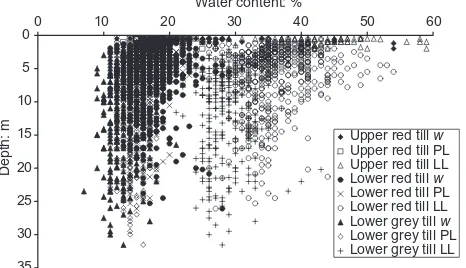
Figure 5 highlights the difficulty in assigning characteris-tic values to this spatially variable soil and identifying the
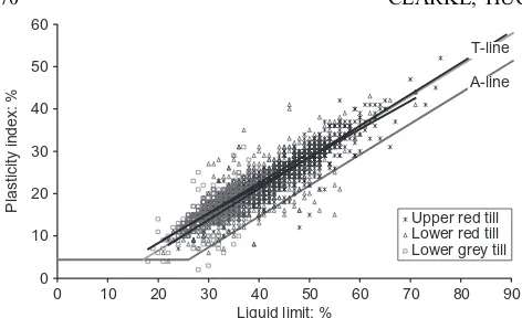
differences between the tills. Note that the amount of data available reduces with depth. The data from all the sites in this study have been plotted on the Casagrande plot in Fig. 6. Soils of similar composition tend to lie on lines parallel to the A-line; Boulton (1976) suggested that clay-matrix-dominant tills of the UK cluster about the T-line. Fig. 6 SCOTLAND
NORTHUMBERLAND
CUMBRIA
COUNTY DURHAM
TYNE & WEAR
NEWCASTLE UPON TYNE
DURHAM Oughterside
Maryport DP
Linefoot Foxhouse South Broughton Lodge Potatopot Lostrigg Workington
Keekle Extension Moresby
Chester House Acklington
Coldrife East Chevington Maiden’s Hall
Stobswood Butterwell
Widdrington DP Butterwell DP Linton Lane West Linton Colliersdean
Hathery Lane
Hunters Moor Bebside
Red Barns
Whitwell
Hill Top
[image:4.595.46.539.51.468.2]Herrington Colliery
Fig. 4. Location of opencast pits in the North of England (after Hashemiet al., 2006). This paper used the data from the sites in Northumberland
60 50 40 30 20 10 0
5
10
15
20
25
30
35 0
Water content: %
Depth: m
Upper red tillw Upper red till PL Upper red till LL Lower red tillw Lower red till PL Lower red till LL Lower grey tillw Lower grey till PL Lower grey till LL
Fig. 5. Profile of Atterberg limits and water content for a site in North East England
[image:4.595.304.537.527.661.2]shows that both these statements apply, which suggests that the three tills have a similar composition, though the particle distribution differs between the tills.
The average Atterberg limits from samples obtained at 0.5 m intervals (upper red till) and 1 m intervals (lower tills) have been plotted in Fig. 7, which also shows that other tills from the UK lie on or adjacent to the T-line. Boulton & Paul (1976) showed that the Atterberg limits tended to fit on a line parallel to the A-line, known as the T-line. The fact that soils from across the country appear to have the same composition is, in part, due to the fact that reworking the tills during successive periods of glaciation has ensured that source material has been widely distributed.
The volume of data allows a statistical analysis to be undertaken to establish whether the data from different sites have the same characteristics of the master set, and whether a characteristic range of values can be identified. Atterberg limits for the three tills are presented in the form of histograms in Fig. 8. The three sets of data create over-lapping but distinctly skewed distributions. There are a significant number of outliers shown in Fig. 8, which are defined as those that are less than or greater than twice the standard deviation from the mean. Cherbyshev’s rules imply that 85% of the results will lie within two standard devia-tions of the mean. Removing the outliers improves the normality of the data.
[image:5.595.58.294.46.190.2]Box plots (Fig. 9) are a visual means of assessing the normality of the data. The median is the data point in the middle of a box that represents the samples between the first and third quartile. The extensions from the boxes represent the limits to the data used in subsequent analyses. Note that less than 4% of the data, which have been removed, were outliers.
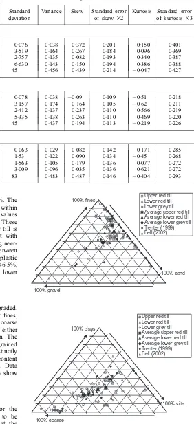
Table 1 lists the descriptive statistics for the three tills. This includes the mean and range, and description of the distribution of that range for the unit weight, water content, Atterberg limits and undrained shear strength. The range is expressed in terms of the mean, and first and third quartiles. The description of the distribution is expressed in terms of the standard deviation and variance. Skew and kurtosis have been used to determine the appropriate statistical techniques to be used to produce the characteristic and baseline values.
It shows that the average plastic limits in the area are
20.3% (6.6%), 17.6% (5.4%) and 14.8% (4.1%) for the
upper and lower red tills and grey till respectively, excluding those values that fall outside two standard deviations from the mean. Fifty per cent of the results fall within 2.3%, 1.6% and 1.1% of the mean. The values for liquid limit are
46.5% (15.5%), 38.7 (12.3%) and 31.3% (6.7%), with
90 80 70 60 50 40 30 20 10 0 10 20 30 40 50 60 0
Liquid limit: %
Plasticity inde
x: %
Upper red till Lower red till Lower grey till
A-line T-line
Fig. 6. Casagrande plot for the tills, showing the relationship between their limits and the T-line, a line parallel to the A-line (the best-fit lines for each till are shown as dashed lines)
90 80 70 60 50 40 30 20 10 0 10 20 30 40 50 60 0
Liquid limit: %
Plasticity inde
x: %
Trenter (1999) Bell (2000) Upper red till Lower red till Lower grey till
Fig. 7. Casagrande plots for UK tills, showing they tend to align with the T-line
40 38 36 34 32 30 28 26 24 22 20 18 16 14 12 10 72 68 64 60 56 52 48 44 40 36 32 28 24 20 16 12 0 100 200 300 400 500 600
0 2 4 6 8
Plastic limit: %
Number
Upper red till Lower red till Lower grey till
0 100 200 300 400 500 600
0 4 8
Liquid limit: %
Number
[image:5.595.315.550.57.358.2]Upper red till Lower red till Lower grey till
Fig. 8. Distribution of (a) plastic limit and (b) liquid limit for upper and lower red tills and grey till
0 5 10 15 20 25 30 35 40 45 50 All limits Hather y LaneBebside Linton LaneStobs wood WiddringtonCollier sdean
Maiden HallAc
klington
[image:5.595.316.551.412.552.2]Plastic and liquid limit: %
Fig. 9. Box plots for lower grey till with outliers removed to highlight the engineering significance of the data from the various sites
[image:5.595.60.293.610.750.2]50% of the results falling within 4.5%, 3.7% and 2.3%. The mean value of plastic limit for each of the sites is within 2.8%, 2.1% and 1.9% of the overall mean; and the values for the liquid limit are within 4.9%, 6.7% and 2.7%. These data show that the spatial variability of the lower grey till is less than that of the upper tills, which is consistent with increased deformation prior to deposition. From an engineer-ing point of view the differences in Atterberg limits between the sites are not significant: hence the mean values of plastic limit and liquid limit in the area are 20.3% : 46.5%, 17.6% : 38.7% and 14.8% : 31.6% for the upper and lower red till and grey till respectively.
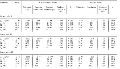
Particle size distribution
[image:6.595.45.538.73.389.2]Clay-dominant subglacial tills are generally well graded. Fig. 10 shows ternary diagrams for the percentages of fines, sands and gravel (Fig. 10(a)) and clay, silt and coarse particles (Fig. 10(b)). Note that cobbles are removed either in the sampling process or in preparing the specimen. The gradings confirm that the tills are dominated by fine-grained particles. The averages show that the tills are distinctly different. Fig. 10(b) shows that, on average, the clay content decreases and the sand content increases with depth. Data from Trenter (1999) and Bell (2002) are included to show the variation in gradings of UK tills.
Water content
The average water content at intervals of 1 m for the lower tills and 0.5 m for the upper red till tends to be constant with depth (Fig. 11). This graph shows that the average water content is greater than the plastic limit for the upper red till; approximately equal to the plastic limit for the lower red till; and lower than the plastic limit for the lower grey till.
The average water contents in the area are 21.5%
(10.4%), 18.1% (7.2%) and 12.5% (3.9%) for the
upper and lower red tills and grey till respectively (Table 2),
excluding those values that fall outside two standard devia-tions from the mean. Fifty per cent of the results fall within 2.5%, 2.1% and 1.2% of the mean. The outlying values are attributed to local pockets of wetter materials, and sample Table 1. Descriptive statistics for the regional database after all outliers removed
Parameter Range Description of distribution
Mean Number of
data points 1st quartile
2nd quartile
Standard deviation
Variance Skew Standard error
of skew 32
Kurtosis Standard error
of kurtosis 33
Upper red till
ªb: Mg/m3 2.06 596 1.95 2.05 0.076 0.038 0.372 0.201 0.150 0.401
w: % 21.5 706 19.0 23.7 3.519 0.164 0.267 0.184 0.096 0.369
PL: % 20.3 641 18.0 22.0 2.757 0.135 0.082 0.193 0.340 0.387
LL % 46.5 637 42.0 51.0 6.630 0.143 0.150 0.194 0.386 0.388
cu: kPa 99 526 65 125 45 0.456 0.439 0.214 0.047 0.427
Lower red till
ªb: Mg/m3 2.06 2024 2.01 2.12 0.078 0.038 0.09 0.109 0.51 0.218
w: % 18.1 2157 16.0 20.0 3.157 0.174 0.164 0.105 0.62 0.211
PL: % 17.6 2000 16.0 19.0 2.412 0.137 0.237 0.110 0.566 0.219
LL % 38.7 1978 35.0 42.0 5.335 0.138 0.263 0.110 0.469 0.220
cu: kPa 100 1879 68 127 45 0.437 0.194 0.113 0.219 0.226
Lower grey till
ªb: Mg/m3 2.18 1185 2.13 2.22 0.063 0.029 0.082 0.142 0.171 0.285
w: % 12.5 1341 11.3 13.6 1.53 0.122 0.090 0.134 0.45 0.268
PL: % 14.9 1296 14 16 1.563 0.105 0.179 0.136 0.077 0.272
LL % 31.3 1293 29 33 3.009 0.096 0.035 0.136 0.621 0.272
cu: kPa 172 1121 111 231 83 0.483 0.487 0.146 0.404 0.293
Upper red till Lower red till Lower grey till Average upper red till Average lower red till Average lower grey till Trenter (1999) Bell (2002)
100% gravel
100% sand 100% fines
Upper red till Lower red till Lower grey till Average upper red till Average lower red till Average lower grey till Trenter (1999) Bell (2002)
100% coarse
100% silts 100% clays
Fig. 10. Ternary plots for UK glacial tills highlighting variation in the tills according to: (a) fines; (b) clays
[image:6.595.256.538.84.701.2]disturbance. The average water contents for each site are within 1.7%, 2.5% and 0.5% of the mean of all sites, suggesting that the average values of water content in the area are 21.5%, 18.1% and 12.5%.
Density
There is a trend of increasing average density with depth, though the increase over the full profile is about 10% of the average value for each till (Fig. 12). The
average bulk densities in the area are 2.00 Mg/m3
(0.20 Mg/m3), 2.06 Mg/m3 (0.18 Mg/m3) and 2.18 Mg/
m3 (0.17 Mg/m3) for the upper and lower red tills and
grey till respectively (Table 2), excluding those values that fall outside two standard deviations from the mean. Fifty
per cent of the results fall within 0.05 Mg/m3 of the mean
for all the tills. The outlying values are attributed to local pockets of wetter materials, sample disturbance and signifi-cant gravel content. The average bulk densities for each site
are within 0.08 Mg/m3, 0.27 Mg/m3 and 0.07 Mg/m3 of the
mean of all sites, suggesting that the average values of bulk
density in the area are 2.00 Mg/m3, 2.06 Mg/m3 and
2.18 Mg/m3, though in the 10 m where the majority of
construction takes place the average values are 2.00 Mg/m3,
2.05 Mg/m3 and 2.15 Mg/m3.
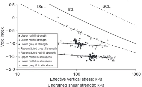
Shear strength
The derived undrained shear strength is considered here as a classification parameter. Fig. 13(a) shows that the strength is spatially variable. The scatter in the data is due to the variation in composition, water content, fabric (e.g. the tills are fissured and, in places, weakly laminated) and sample disturbance, as well as in situ effective stress. The average values at a given depth (0.5 m intervals for the upper red till and 1 m intervals for the lower tills) have been plotted in Fig. 13(b), provided there were at least five samples tested at that depth. The alternative was to consider the average strength of adjacent samples in each borehole, assuming that the random distribution was localised. This removed those 50
45 40 35 30 25 20 15 10 5 0
5
10
15
20
25
30
35
40 0
Water content: %
Depth: m
Upper red tillw
Upper red till PL Upper red till LL
Lower red tillw
Lower red till PL Lower red till LL
Lower grey tillw
[image:7.595.61.297.57.186.2]Lower grey till PL Lower grey till LL
[image:7.595.319.553.57.190.2]Fig. 11. Variation of average water content and Atterberg limits with depth
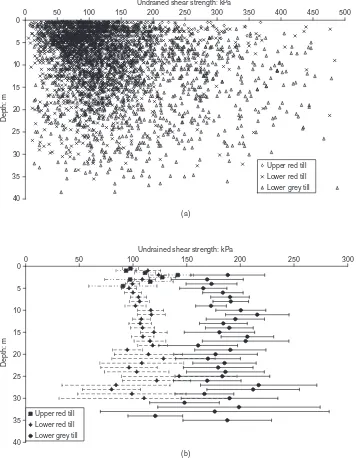
Table 2. Characteristic values from the regional database
Parameter Mean Characteristic values Baseline values
Schneider (low)
Cautious mean (low)
Cautious mean (high)
Student-t factor for
95%
k Minimum Maximum Student-t
factor for 95%
k
Upper red till
ªb: Mg/m3 2.00 1.960 1.993 2.003 1.646 0.067 1.87 2.12 1.64 1.646
w: % 21.5 19.74 21.28 21.72 1.646 0.062 15.7 27.3 1.64 1.645
PL: % 20.3 18.98 20.17 20.53 1.646 0.065 15.8 24.9 1.64 1.645
LL % 46.5 43.18 46.06 46.93 1.646 0.065 35.6 57.4 1.64 1.645
cu: kPa 99 76 96 102 1.646 0.072 24 173 1.64 1.646
Lower red till
ªb: Mg/m3 2.06 2.023 2.059 2.065 1.646 0.037 1.93 2.19 1.64 1.642
w: % 18.1 16.56 18.02 18.25 1.646 0.035 13.0 23.3 1.64 1.642
PL: % 17.6 16.39 17.51 17.69 1.646 0.037 13.6 21.6 1.64 1.642
LL % 38.7 36.02 38.49 38.89 1.646 0.037 29.9 47.4 1.64 1.642
cu: kPa 100 78 98 101 1.646 0.038 38 171 1.64 1.642
Lower grey till
ªb: Mg/m3 2.18 2.145 2.173 2.179 1.646 0.048 2.07 2.28 1.64 1.643
w: % 12.5 11.77 12.46 12.60 1.646 0.045 10.0 15.0 1.64 1.642
PL: % 14.9 14.08 14.79 14.94 1.646 0.046 12.3 17.4 1.64 1.643
LL % 31.3 29.78 31.15 31.43 1.646 0.046 26.3 36.2 1.64 1.643
cu: kPa 172 131 168 176 1.646 0.049 35 310 1.64 1.643
2·4 2·3 2·2 2·1 2·0 1·9 1·8 1·7 1·6 1·5 0
5
10
15
20
25
30
35
40 1·4
Density: Mg/m3
Depth: m
Upper red till bulk density Upper red till dry density Lower red till bulk density Lower red till dry density Lower grey till bulk density Lower grey till dry density
Fig. 12. Variation of average bulk and dry density with depth
[image:7.595.57.566.486.780.2]samples that had no adjacent samples, and reduced the scatter, but there was no significant improvement in the quality of the profile. Both methods showed that there was no clear trend of change of strength with depth.
Table 2 shows that the average undrained strengths for the three tills in the area are 115 kPa, 110 kPa and 185 kPa after the outliers exceeding two standard deviations have been removed. The ranges have not been presented, as the upper bound is more than twice the average strength. Fifty per cent of the results fall within one standard deviation of the average. The mean undrained shear strength for each site is within 25 kPa, 25 kPa and 60 kPa of the mean of all sites.
DISCUSSION
These results can be used to produce characteristic pro-files with depth for preliminary designs, characteristic and baseline values for design and construction, and a means of enhancing further investigations.
Modelling of the till
In order to assign characteristic values to the till it is necessary to produce a model to establish whether there is a trend in the data. This can be a deterministic model based on empirical or theoretical relationships, a stochastic model based on a statistical analysis of the data, or a combination of these. The former includes relationships between the Atterberg limits and undrained shear strength of remoulded clays (e.g. Wroth & Wood, 1976; Carrier and Beckman, 1984); in situ strengths of normally consolidated clays, density and Atterberg limits (e.g. Skempton, 1957); and overconsolidated soils and Atterberg limits (e.g. Yilmaz, 2000). Burland (1990) and Chandler (2000) suggested that the intrinsic properties of a soil can provide a framework to characterise clay. This framework is shown in Fig. 14, in which the average shear strength for each till taken from
Fig. 13 is plotted against the void index,Iv, given by
Iv¼
ee100
Cc (1)
500 450 400 350 300 250 200 150 100 50
300 250
200 150
100 50
(a)
(b) 0
5
10
15
20
25
30
35
40 0
Undrained shear strength: kPa
Depth: m
Depth: m
Upper red till
Lower red till Lower grey till
0
5
10
15
20
25
30
35
40 0
Undrained shear strength: kPa
Upper red till
Lower red till
[image:8.595.113.469.55.513.2]Lower grey till
Fig. 13. Variation in undrained shear strength with depth for all sites showing: (a) all data; (b) mean and characteristic strengths at each depth
where e100 is the void ratio at a vertical effective stress of
100 kPa on the intrinsic compression line, and Cc is the
slope of the intrinsic compression line. Burland (1990) suggested that these two intrinsic properties are empirically
related to the void ratio at the liquid limiteL by
e100¼0:114þ0:581eL (2)
Cc ¼0:256eL0:04 (3)
The intrinsic compression line, ICL, represents the compres-sion curve for reconstituted clays; the intrinsic strength line, ISuL, represents the strength of reconstituted soils (Chandler, 2000). Fig. 14 shows that results of tests on reconstituted
tills (Clarkeet al., 1998) fit to the ISuL, which suggests that
this framework can be used to characterise the tills.
The average void index, vertical effective stress and shear strength for the three tills are plotted in Fig. 14. The void indices plotted against the in situ effective vertical stress for the upper and lower red till lie to the left of the ISuL, confirming that they are overconsolidated and, since they lie about a common line, suggests that they have had a similar stress history, leading to the conclusion that they are a single till, the difference being the weathering in the upper red till. The lower grey till is also overconsolidated, but the precon-solidation pressure exceeds that of the red till. The best fit to the data are two lines that are very nearly parallel. The slope of the lines is such that the average void ratio is very nearly constant, which implies that the characteristic shear strength profile could be considered to be vertical (see Fig. 13): hence the reason why the strengths cluster about two points in Fig. 14.
Characteristic values
[image:9.595.59.296.49.194.2]The evidence from this database is that the classification parameters are random, reflecting the composition and fabric of the tills and depositional and post-depositional processes. Fig. 11 shows that the mean values of Atterberg limits and water content for each till are reasonably uniform with depth, so the values given in Table 2 represent the regional mean values. Note that the apparent trend shown in Fig. 5 is due to the reduction in the amount of data with depth. This is the reason for the increased variation from the mean in Fig. 11.
Figure 12 shows that the regional average density in-creases with depth. Fig. 13 shows that the regional average shear strength shows no trend with depth: therefore an average value can be used for classification purposes.
This regional database represents a ‘global’ situation: therefore a cautious mean represents the characteristic value
(Frank et al., 2004), with the probability of the worst case
occurring being less than 5%. Frank et al. (2004) suggest
that, if there no significant trend in the data, the
character-istic value Xk is given by
Xk ¼Xmeanð1knVxÞ (4)
Xk .Xmean is used when the cautious mean is a high value,
for example when calculating active pressures on retaining
structures; and Xk , Xmean is used when the cautious mean
is a low value, for example when calculating bearing
capa-city. Vx, the coefficient of variation, is equal to the standard
deviation divided by the mean value if there is no trend to
the data and there is noa priori knowledge. The value ofVx
given in Table 2 can be considered as a prioriknown value
when characteristic values are being derived from a new
investigation in the region. kn is a statistical coefficient that
takes into account the number of samples, the volume of the ground, the type of results, and the level of confidence.
Schneider (1999) suggested that the characteristic value for a new investigation is simply the mean less half the standard deviation, since the regional coefficient of variation is likely to be unknown. Table 2 shows that this can lead to a characteristic value, with about 70% of the results exceed-ing that value: that is, it is an over-cautious estimate of the mean.
The characteristic values for design may be different from baseline values for construction, since baseline values are established for contractual reasons to limit claims arising from unforeseen circumstances (Randall, 1997). The values are based on an assessment of the subsurface conditions to produce rational limits to the likely worst-case values. Given that these govern construction processes, then the local low (or high) value could be considered. Eurocode 7 (2004) suggests that this is represented by the 5% fractile values 1000
100
⫺2·0
⫺1·5
⫺1·0
⫺0·5
0 0·5
10
Effective vertical stress: kPa Undrained shear strength: kPa
Void inde
x
Upper red till strength Lower red till strength Lower grey till strength Reconstituted grey till strength Reconstituted red till strength Upper red till in situ stress Lower red till in situ stress Lower grey till in situ stress
ICL
ISuL SCL
Fig. 14. Relationship between intrinsic compression and
strength lines and in situ conditions and shear strength
90 80 70 60 50 40 30 20 10
1000 100
0 10 20 30 40 50 60
0
Liquid limit: % (a)
Plasticity inde
x: %
Upper red till Lower red till A-line T-line
⫺2·0
⫺1·5
⫺1·0
⫺0·5
0 0·5
10
Effective vertical stress: kPa Undrained shear strength: kPa
(b)
Void inde
x
Upper till in situ stress Lower till in situ stress Upper till strength Lower till strength ICL
ISuL SCL
Red till from regional database
Grey till from regional database
Fig. 15. Relationships between (a) classification data and the T-line and (b) intrinsic compression and strength lines and in situ conditions for the new dataset
[image:9.595.319.550.424.740.2]that are given in Table 1. In this case kn in equation (4) is
1.64ˇ(1/n +1).
Application to other investigations
An aim of this study is to develop a protocol that could be used to assign characteristic and baseline values to a till. In that case it has to be shown that a set of data from a new site investigation in the region has characteristics that fit those of the regional database. The Atterberg limits for the tills identified at a new site in the region lie about the T-line, confirming the geologist’s description of glacial till (Fig. 15(a)). Tests for skew and kurtosis of the local dataset show that normality can be assumed (Table 3). The majority of the data lie to the left of the ISuL and about the trend for the red till from the regional database. The scatter in the data reflects the nature of till, but a combination of the geological history, description and classification character-istics suggests that the till that forms the new dataset is the red till identified in the regional database.
It is therefore possible to use Bayesian statistics to determine the characteristic and baseline values. The mean value, standard deviation and variance of the new database,
taking into account the regional database and the local dataset, are derived from
ì2¼
n1x1ó20þì0ó21
n1ó20þó21 (5)
ó2¼
ffiffiffiffiffiffiffiffiffiffiffiffiffiffiffiffiffiffiffiffiffi ó20ó21
n1ó20þó21 s
(6)
s22¼
1 1=s1
0þ1=s21
(7)
wheres2,ó2 and ì2 are the variance, standard deviation and
mean of the total distribution; s1,ó1 andx1 are the variance,
standard deviation and mean of the new data; s0,ó0 and ì0
are the variance, standard deviation and mean of the regional
database; andn1 is the number of new datasets.
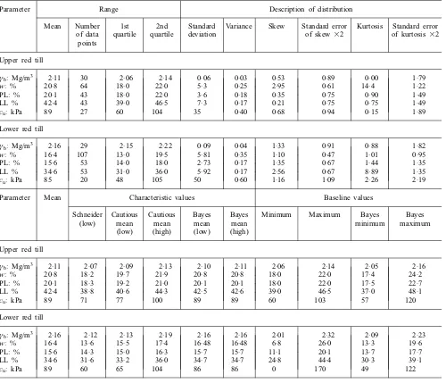
The descriptive statistics for the new dataset are given in Table 3, together with the characteristic and baselines values
based on the dataset and ona prioriknowledge. This shows
that the inclusion of a priori knowledge has resulted in less
[image:10.595.43.543.71.500.2]cautious design and construction parameters and hence a more economic design.
Table 3. Descriptive statistics and characteristic values for the new dataset
Parameter Range Description of distribution
Mean Number
of data points
1st quartile
2nd quartile
Standard deviation
Variance Skew Standard error
of skew 32
Kurtosis Standard error
of kurtosis32
Upper red till
ªb: Mg/m3 2.11 30 2.06 2.14 0.06 0.03 0.53 0.89 0.00 1.79
w: % 20.8 64 18.0 22.0 5.3 0.25 2.95 0.61 14.4 1.22
PL: % 20.1 43 18.0 22.0 3.6 0.18 0.35 0.75 0.90 1.49
LL % 42.4 43 39.0 46.5 7.3 0.17 0.21 0.75 0.75 1.49
cu: kPa 89 27 60 104 35 0.40 0.68 0.94 0.15 1.89
Lower red till
ªb: Mg/m3 2.16 29 2.15 2.22 0.09 0.04 1.33 0.91 0.88 1.82
w: % 16.4 107 13.0 19.5 5.81 0.35 1.10 0.47 1.01 0.95
PL: % 15.6 53 14.0 18.0 2.73 0.17 1.35 0.67 1.44 1.35
LL % 34.6 53 31.0 36.0 5.92 0.17 2.56 0.67 8.89 1.35
cu: kPa 85 20 48 105 50 0.60 1.16 1.09 2.26 2.19
Parameter Mean Characteristic values Baseline values
Schneider (low)
Cautious mean (low)
Cautious mean (high)
Bayes mean (low)
Bayes mean (high)
Minimum Maximum Bayes
minimum
Bayes maximum
Upper red till
ªb: Mg/m3 2.11 2.07 2.09 2.13 2.10 2.11 2.06 2.14 2.05 2.16
w: % 20.8 18.2 19.7 21.9 20.8 20.8 18.0 22.0 17.4 24.2
PL: % 20.1 18.3 19.2 21.0 20.1 20.1 18.0 22.0 17.5 22.7
LL % 42.4 38.8 40.6 44.3 42.5 42.6 39.0 46.5 37.0 48.1
cu: kPa 89 71 77 100 89 89 60 103 57 120
Lower red till
ªb: Mg/m3 2.16 2.12 2.13 2.19 2.16 2.16 2.01 2.32 2.09 2.23
w: % 16.4 13.6 15.5 17.4 16.48 16.48 6.8 26.0 13.3 19.6
PL: % 15.6 14.3 15.0 16.3 15.7 15.7 11.1 20.1 13.7 17.7
LL % 34.6 31.6 33.2 36.0 34.7 34.7 24.8 44.4 30.3 39.1
cu: kPa 89 60 65 104 86 86 0 170 49 122
CONCLUSIONS
Glacial tills, which cover some 60% of the UK and are some of the most widely distributed deposits in the world, are difficult to characterise owing to the variation in fabric and composition created by the deposition and post-deposi-tional processes. This is accompanied by the difficulty of obtaining quality samples, which means the samples may not be truly representative of the till. Most of the tills in the UK are lodgement or deformation tills, which are hetero-geneous mixtures of clays, silts, sands, gravels, cobbles and boulders. They are clay-matrix-dominant tills such that their behaviour is often considered to be that of clay. The Atter-berg limits of the fines content show that the composition of the UK tills is similar, as they lie about a line parallel to the A-line on the Casagrande chart.
In the North East of England there is a tripartite succes-sion of tills that is typical of many UK tills. A study of the intrinsic properties shows that the tills can be considered to be heavily overconsolidated, with the lower grey till being more overconsolidated than the upper red till. The upper red till is divided into two, but a study of the intrinsic properties suggests that the top few metres are weathered red till.
A statistical analysis of a regional database shows that for design and construction purposes the physical characteristics of each till (treating the upper and lower red tills as separate for this purpose) can be assumed to be constant with depth until proven otherwise. The lower grey till is generally denser and stiffer than the upper red till. Both tills can be classed as inorganic clays, with the grey till being less plastic than the red till.
Characteristic values for design for the region have been derived using the method recommended by Eurocode 7 (2004), assuming a 95% probability that these are the worst case likely to be encountered. Baseline values for construc-tion have been developed for the 5% fractile assuming that these would be the worst cases likely to be locally
encoun-tered. These data provide a priori knowledge for future
investigations.
REFERENCES
Beaumont, P. (1968). A history of glacial research in Northern
England from 1860 to the present day. University of Durham, Department of Geography, Occasional Paper No. 9.
Bell, F. G. (2002) The geotechnical properties of some tills
occur-ring along the eastern areas of England. Engng Geol. 63, Nos
1–2, 49–68.
Boulton, G. S. (1976). Some relations between the genesis of tills
and their geotechnical properties. In Glacial till: An
interdisci-plinary study (ed. R. F. Legget). Ottawa: Royal Society of Canada.
Boulton, G. S. & Paul, M. A. (1976). The influence of genetic
processes on some geotechnical properties of glacial tills, Q. J.
Engng Geol.9, No. 3, 159–194.
Burland, J. B. (1990). Thirtieth Rankine Lecture: On the
compressi-bility and shear strength of natural clays.Ge´otechnique40, No.
3, 329–378.
Carrier, W. D. & Beckman, J. F. (1984). Correlations between index
tests and the properties of the remoulded clays. Ge´otechnique
34, No. 2, 211–228.
Carruthers, R. G. (1953). Glacial drift and the under melt theory.
Newcastle upon Tyne: Harold Hill.
Chandler, R. J. (2000). Clay sediments in depositional basins: the
geotechnical cycle. 3rd Glossop Lecture. Q. J. Engng. Geol.
Hydrol.33, No. 1, 5–39.
Clarke, B. G., Chen, C.-C. & Aflaki, E. (1998). Intrinsic
compres-sion and swelling properties of glacial till. Q. J. Engng Geol.
Hydrol.31, No. 3, 235–246.
Eurocode 7 (2004).Geotechnical design, Part 1: General rules, EN
1997-1, Brussels: European Committee for Standardisation (CEN).
Eyles, N. & Sladen, J. A. (1981). Stratigraphy and geotechnical properties of weathered lodgement till in Northumberland,
Eng-land.Q. J. Engng Geol.14, No. 2, 129–141.
Frank, R., Bauduin, C., Driscoll, R., Kavvadas, M., Krebs Ovesen,
N., Orr, T. & Schuppener, B. (2004). Designer’s guide to EN
1997-1 Eurocode 7: Geotechnical design – General rules. London: Thomas Telford.
Hart, J. K. & Boulton, G. S. (1991). Interrelation of glaciotectonic and glaciodepositional processes within the glacial environment. Quaternary Science Reviews10, No. 4, 335–350.
Hashemi, S., Hughes, D. B. & Clarke, B. G. (2006). The character-istics of glacial tills from Northern England derived from a
relational database.Geotech. Geol. Engng24, No. 4, 973–984.
Hughes, D. B., Clarke, B. G. & Money, M. S. (1998). The glacial
succession in lowland Northern England. Q. J. Engng Geol.
Hydrol.31, No. 3, 211–234.
Randall, J. (ed.) (1997). Geotechnical baseline reports for
under-ground construction: Guidelines and Practices. Reston, VA: Technical Committee of the Underground Technology Council, American Society of Civil Engineers.
Robertson, T. L., Clarke, B. G. & Hughes, D. B. (1994).
Geotechni-cal properties of Northumberland Till. Ground Engng 27, No.
10, 29–34.
Schneider, H. R. (1999). Definition and determination of
character-istic soil properties. Proc. 14th Int. Conf. Soil Mech. Geotech.
Engng, Hamburg,4, 2271–2274.
Skempton, A. W. (1957). Discussion on the planning and design of
the new Hong Kong airport.Proc. Inst. Civ. Engrs7, 305–307.
Trenter, N. A. (1999). Engineering in glacial tills, CIRIA Report
No. C504. London: Construction Industry Research and Infor-mation Association.
Wroth, C. P. & Wood, D. M. (1976). The correlation of index
properties with some basic engineering properties of soils. Can.
Geotech. J.15, No. 2, 137–145.
Yilmaz, I. (2000). Evaluation of shear strength of clayey soils by using
their liquidity index.Bull. Engng Geol. Environ.59, 227–229.