CFD modelling of flow characteristics in micro shock tubes

Journal of Applied Fluid Mechanics, Vol. 10, No. 4, pp. 1061-1070, 2017. Available online at www.jafmonline.net, ISSN 1735-3572, EISSN 1735-3645. DOI: 10.18869/acadpub.jafm.73.241.27474

CFD Modelling of Flow Characteristics in Micro Shock

Tubes

A. Mukhambetiyar

_{, M. Jaeger}

_{and D. Adair}

1 _{School of Engineering, Nazarbayev University, Astana, 010000, Republic of Kazakhstan} 2 _{School of Engineering & ICT, University of Tasmania, Hobart, TAS7001, Australia}

†Corresponding Author Email: [email protected] (Received December 8, 2016; accepted April 12, 2017)

A

The use of micro shock tubes has become common in many instruments requiring a high velocity and temperature flow field, for example in micro-propulsion systems and drug delivery devices for medical systems. A shock tube has closed ends, and the flow is generated by the rupture of a diaphragm separating a driver gas at high pressure from a driven gas at relatively low pressure. The rupture results in the movement of a shock wave and contact discontinuity into the low-pressure gas, and an expansion wave into the high pressure gas. The characteristics of the resulting unsteady flow for micro shock tubes are not well known as the physics of such tubes includes additional phenomena such as rarefaction and complex viscous effects at low Reynolds numbers. In the present study, computational fluid dynamics (CFD) calculations are made for unsteady compressible flow within a micro shock tube using the van-Leer MUSCL scheme and the two-layer - turbulence model. Novel results have been obtained and discussed of the effects of using different diaphragm pressure ratios, shock tube diameters and wall boundary conditions, namely no slip and slip walls.

Keywords: Shock wave propagation; Shock wave reflection; Computational Fluid Dynamics; Micro shock tube; Slip wall.

NOMENCLATURE

non-dimensional pressure gradient CS contact surface

diameter EH expansion head

driver section diameter driven section diameter total energy per unit mass

, radial, axial body forces

ℎ enthalpy

Boltzmann constant Kn Knudsen number

length driver section length driven section length

, monitoring positions

M Mach number (shock wave)

M Mach number (contact surface)

, pressure (static) Pr pressure ratio

, radial, axial heat flux

Re Reynolds number radial coordinate S scaling factor

sutherland constant SW Shock wave

temperature reference temperature time

, radial, axial velocities axial distance axial coordinate

thermal accommodation coefficient

momentum accommodation coefficient mean free path

distance from cell centre to wall molecular viscosity

reference viscosity density

Lennard-Jones length

1. I

Micro shock tubes are used in many engineering

shock front and associated expansion and contraction waves by the sudden expansion of gas from a high pressure environment to a low pressure environment. The high pressure and low pressure regions are first separated by a diaphragm which then ruptures, resulting in a shock wave with the flow behind the shock wave induced to move by the shock wave propagation.

The small flow dimension of a shock tube introduces additional flow physics, in particular, micro shock tubes experience shock attenuation from significant viscous effects at low Reynolds numbers. In addition, at high Knudsen numbers, there is slipping of the near-wall fluid due to non-continuum effects, and this acts to increase shock strength and aid shock wave propagation.

Due to the low pressure and micro scale, viscous and rarefaction effects are greatly increased and this makes calculations and experimental results of the shock wave propagation and flow characteristics deviate from theoretical analysis (Zhang et al. 2015). However, a proper understanding of the shock propagation and associated flow field is important to determine fluid or particle momentum and efficiency of the device. In some devices knowledge of the temperature field is necessary to examine efficiency. It is well known that the limit for the continuum based simulations and molecular approaches are defined using a non-dimensional number called the Knudsen number (Kn) (Karniadakis and Beskok 2002), which is the ratio of the mean free path to the flow diameter. A low Knudsen numbers of below 0.01 indicates that continuum approaches are suitable for flow simulations. If the Kn is between 0.01 and 0.1, then Navier-Stokes equations with slip wall boundary conditions represent the flow field very well. If Kn is greater than 0.1, simulations should be carried out using pure molecular approaches. In summary the higher the Knudsen number then the higher the mean free path which subsequently increases the molecular forces. Much work has already been done on macro tubes, starting with an experimental study by Duff (1959) who studied the viscous loss associated with the boundary layer growth in shock propagation. The decelerating shock front and the accelerating contact surfaces eventually lead to a stage where the shock-contact interface tends to a constant value and moves with the same speed. Analytical modelling has been carried out by Mirels (1963) on the effect of boundary layer on shock wave propagation and Brouillete (2003) has proposed a scaling factor, S, which relates tube diameter and initial pressure to the shock attenuation. Diffusive effects of the friction and heat conduction were studied at low values of S in micro shock tubes and the results showed that the model predicted the shock wave at small scale to experience much loss in strength. Sturtevant and Okamura (1969) and Kohsuke et al. (2009) investigated the influence of the boundary layer on the shock wave propagation at different boundary conditions and good agreement was observed between simulations and theoretical results for the laminar region of the boundary layer. The wall

propagation have been studied (Ngomo et al. 2010) and it was found that diffusive shear stresses and energy losses near the wall significantly led to shock wave attenuation.

The application of unsteady Navier-Stokes equations coupled with the velocity slip and temperature jump boundary conditions has been applied to micro tube flows (Zeitoun et al. 2009; Zeitoun and Burtschell 2006), with a strong decrease in the shock strength and flow velocity along the micro shock tube observed. The decay of shock wave strength was much stronger at lower initial pressure and small tube diameter. Based on the Knudsen number, computational studies to investigate the shock wave propagation under different pressure ratios, shock tube diameters with slip condition and no slip wall boundary conditions have been carried out (Arun and Kim 2012a; Arun and Kim 2012b). The results indicated shock wave propagation is attenuated by viscous boundary layer formation, and the decay of the shock wave increases drastically with reduction in diameter.

The choice made here for discretization was the van-Leer MUSCL scheme as opposed to a Riemann solver or an approximate Riemann solver (Roe 1981). This scheme, was one of many oscillation-free higher-order advection schemes launched in an effort to circumvent Godunov’s theorem (1959) which stated that to preserve monotonicity of the solution, the advection scheme should be at most first-order accurate. van-Leer (1984) regarded oscillations as the result of oscillatory interpolation of the discrete initial values and proposed the remedy therefore as consisting of introducing monotonicity-preserving interpolation. The simplest higher-order schemes reconstruct a linear or quadratic distribution in a cell using three contiguous cell averages. Following Godunov (1959) van-Leer’s schemes included fluxes derived from the solution of Riemann problems and when combined with higher-order reconstruction this led to upwind-biased differencing, hence the name MUSCL - Monotone Upstream Scheme for Conservation Laws. There is evidence from the review by Woodward and Colella (1984) that superior shock capturing ensues from such a high-resolution Godunov-type method, and so it was chosen for this work.

The objective of the present study is to numerically simulate unsteady flow evolution, shock propagation and shock reflection inside a micro shock tube. Effects of different diaphragm pressure ratios are investigated and effects of the shock tube diameter on shock wave and contact surface propagation are also investigated. Different wall boundary conditions of no slip and slip walls were used to observe unsteady flow characteristics. The scaling parameter

S indicating effects of the scale was calculated.

2. M

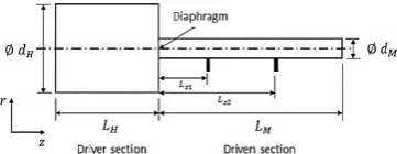
initialized at high pressure and the driven section is kept at low pressure. Due to the pressure difference between driver and driven sections, when the diaphragm is ruptured instantaneously, the normal shock wave develops and moves towards the driven section. As the shock wave meets the end wall of the driven section, it is reflected and moves towards the driver section. The positions of two pressure transducers are shown where experimental results were obtained (Andong National University, 2016).

Fig. 1. Schematic of a closed micro shock tube.

3. G

Transient, 2D axisymmetric calculations were made with compressible Navier-Stokes equations coupled with species transport equations to predict the change in flow parameters. The conservation equations used in this work were

Continuity

+1 ( )+ ( )= 0 (1)

Axial Momentum

( )

+1 ( )+1 ( )

= −

+1 2 −2

3(∇ ∙ )

+1 + +

(2)

Radial Momentum

( )

+1 ( )+1 ( )= −

+1 +

+1 2 −2

3(∇ ∙ )

−2 +2

3 (∇ ∙ ) +

(3)

Energy

( )

+1 ( ℎ )+1 ( ℎ ) (4)

= 2 −2

3 ∇ ∙

+ 2

3

(2 − ∇ ∙ )

+ 2 −2

3 ∇ ∙

+ +

+ 1 2 −2

3 ∇ ∙

−2 3

(2 − ∇ ∙ )

+

+

+ 1 +

+ 2 −2

3 ∇ ∙ −

1 ( )

−

where

∇ = + + (5)

is the axial coordinate, is the radial coordinate, is the axial velocity, is the radial velocity, is static pressure, is molecular viscosity, the total energy per unit mass, ℎ is enthalpy, and are the respective radial and axial heat fluxes and is body force.

The total energy per unit mass is evaluated from the total enthalpy per unit mass as

= ℎ − ⁄ (6)

The PHOENICS (Cham 2016) code together with some FORTRAN-coding sequences added through user-accessible subroutines was used for the computation of these equations. The flow was considered turbulent and solved as transient. The ideal gas equation was used to predict the variation of density with respect to temperature and pressure. The higher-order van Leer MUSCL scheme was used for the discretization of convection and a first-order Euler scheme was used for the transient terms. At very low pressure, due to rarefaction the flow no longer attaches to the wall but slips. At these conditions a jump in the near wall fluid temperature can be observed. The slip wall boundary condition was performed at low pressure by using Maxwell’s slip velocity and temperature jump equations, as (Karniadakis 2000)

− = 2 2 − − (8)

=

√2 (9)

Here and are the momentum and thermal accommodation coefficients respectively, and the subscripts , and indicate gas, wall and cell-centre velocities respectively. is the mean free path , is the distance from the cell-centre to the wall, is the Boltzmann constant and is the Lennard-Jones characteristic length of species. The slip velocity is derived from Eq. (7) and the viscosity was modelled as a function of temperature using the Sutherland viscosity model

= +

+ (10)

Here is the viscosity of the gas, is a reference viscosity, is the static temperature and is a reference temperature and is the Sutherland constant.

4. S

The shock wave and contact surface are induced by the ruptured diaphragm. The shock wave and contact surface move toward the driven section with Mach numbers M and M . In an ideal shock tube, at fixed initial conditions, both in driver and driven sections,

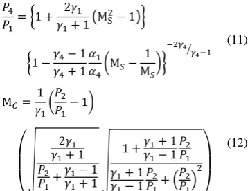
M and M can be calculated as

= 1 + 2

+ 1 MS− 1

1 − − 1

+ 1 M −

1 M

(11)

M = 1 − 1

2 + 1 + − 1_{+ 1}

1 + + 1_{− 1} + 1

− 1 +

(12)

The shock wave Mach number and contact surface Mach number keep constant in micro shock tubes (Zhang et al. 2015) as all boundary conditions are fixed. MS and MC increase with the increase of the

diaphragm pressure ratio. However due to the attenuation which happens in the real shock tube flow resulting from viscous and rarefaction effects, shock wave and contact surface Mach numbers always show a difference from theoretical solutions. The shock wave Mach number gradually decreases, but contact surface Mach number gradually increases. The formation and development of the boundary layer behind the shock wave is the main reason for this (Zhang et al. 2015).

4.1 Scaling Factor S

Heat conduction and shear stresses make remarkable

shock wave behavior in a micro shock tube as demonstrated by Brouillete (2003), where a control volume defined as the region between the shock wave and contact surface was proposed to quantify effects of the scale and diffusive transport phenomena on shock wave propagation as is shown on Fig. 2.

Fig. 2. Control volume used in the study of diffusive effects in the micro shock tube.

SW, CS and EH respectively represent shock wave, contact surface and expansion head. The friction and heat transfer to side walls are described by appropriate source terms through this control volume approach. As the shock wave and contact surface propagate in the driven section, the length of control volume becomes larger due to the velocity difference between the shock velocity and contact surface velocity. Based on the control volume, the scaling parameter S indicating effects of the scale was used as

= 1 + − 1

2 MS 1 −

− 1

S 1

MSPr − 1

(13)

where, S = (Re ) 4⁄ . Reynolds number and the distance are two important variables to calculate S, and the velocity, density and dynamic viscosity of the flow are obtained from the region between the shock wave and contact surface. The effects of the scale are investigated by calculating the Reynolds number and the decrease of the length of . Eq (13) indicates that a smaller S value will have obvious effects on calculating density ratio between the front and back of the shock wave. Lower Reynolds numbers and larger values will contribute to smaller S values. If S becomes infinite, any effects of scaling can be ignored. This happens in shock tubes with large diameters and high Reynolds numbers.

4.2 Pressure Gradient

As a shock wave moves in a micro shock tube, the pressure gradient of the flow in front of and after the shock changes. The pressure gradient is related to the pressure difference in front of and after the shock wave and the distance across the shock wave. As the pressure gradient across a shock is fairly linear, the gradient can be calculated by

≈ −

−

(14)

where − represents the pressure difference across the shock and − is the distance of pressure change across the shock.

= = − −

(15)

It should be noted that the pressure gradient calculation ensuing from Eq. (14) cannot distinguish between expansion and compression shock waves or calculation near a solid wall. This first-order formulation is different from that used in the Navier-Stokes calculations here. For these calculations a MUSCL based scheme was used which extends the idea of using a piecewise approximation to each cell by using limited left and right extrapolated states. This scheme takes the form

∆ − (16)

where the numerical fluxes correspond to a non-linear combination of first- and second-order approximations of the continuous flux function.

5. C

L S

5.1 Validation

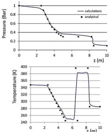
Validation of the computer code was made in two ways. First, 1D transient calculations were made inside a macro shock tube for which there is an analytical solution (Sod 1978). Phenomena such as shock waves, contact discontinuity and rarefaction waves are common to both macro and micro shock tubes but as already stated for micro shock tubes, under the influence of significant viscous effects, and at high Knudsen number, rarefaction effects also come into play. The tube length and time period were chosen so that the calculations end before the waves are reflected from the tube ends. The macro tube was 10m long with a cross-sectional area of 0.1m2 _{and 90}

cells were used to cover the computational domain. In the driver region the initial pressure was set at 1 bar, the temperature at 348.391 K and the gas density at 1.0 kg/m3_{. In the driven region the initial pressure}

was set at 0.1 bar, the temperature at 278.13 K and the gas density at 0.125 kg/m3. The wall friction

effect is ignored and the energy equation solved as static enthalpy with an ideal-gas equation of state. The higher-order van Leer MUSL scheme is used for the discretization of convection and the default first-order Euler scheme is used for the transient terms. As can been seen from Fig. 3, reasonable agreement was found between the calculated and analytical results. The region within the shock was well calculated but just at the beginning and end of the shock were not captured satisfactorily. The van-Leer MUSCL scheme was used here as the default hybrid scheme found in PHOENICS can produce inferior results due to numerical smearing. However it can be seen that proper capture is still not evident due to clipping of the extrema. This may be due to the total variation diminishing (TVD) feature of the MUSCL scheme used, which of course is a serious drawback. To avoid this loss of accuracy near extrema, it seems necessary to satisfy the monotonicity preserving criteria due to Suresh and Huynh (1997) that enlarges the TVD intervals to provide room for the numerical flux to maintain an accurate value. This has already been carried out by Daru and Tenaud (2009) and it

can be concluded that a better discretization scheme, which includes the enlargement of TVD intervals, should be used in future work.

Fig. 3. Macro shock tube results for calculated solution compared to analytical solution at

= . ms.

The second validation method used was comparison with the experimental data of Park et al. (2014) where a micro shock tube with a 6mm diameter and a pressure ratio (Pr) of 6 was used with the driver region initially set at 6 atm and the driven region initially set at 1 atm. The shock wave and expansion wave propogation curves were obtained as shown on Fig. 4 where SW and EH represent the shock wave and expansion head respectively.

Fig. 4. Experimental and calculated results for wave location at different times.

The results show reasonable agreement although generally more attenuation occurred in the experimental study. This is probably due to the fact that real gas shows more viscous effects and there was heat transfer between the shock heated gas and tube walls. The walls were assumed to be adiabatic and held at 300K during the calculations.

5.2 Computational Domain

The computational domain consists of a driver and driven sections as shown on Fig.1. The dimensions used in this work were, the lengths of the driver

( ) and the driven ( ) sections are 41mm and 66mm respectively. The diameters of the driver

( ) and driven ( ) sections are 20mm and 7.5mm respectively. The domain was discretized using a structured, cylinder-polar grid. After performing grid independent solution tests the final grid used 120 radial by 1200 axial cells, of which 60 radial by 720 axial cells are located in the driven section, and 120 radial by 480 axial cells in the driver section. The grid was refined close to solid wall using a geometric progression distribution. This is demonstrated for the region close to the end of the driven region on Fig. 5 where only selected grid nodes are shown to ensure clarity. Each simulation was run for a total of 0.5ms using the uniform time steps given in Table 1. The two-layer - turbulence model mention in Table 1 is that reported by Elhadidy (1980) and Rodi (1991) and uses the high Reynolds number - turbulence model away from the walls in the fully turbulent region while the near-wall viscosity-affected layer is resolved with a one-equation model involving a length-scale prescription (Norris and Reynolds 1975). During the calculations, no under-relaxation factors were used and the maximum residual for each variable was set at 10-4 _{to achieve}

convergence. Each case was computed on a Dell 5500 Workstation with an Intel Xeon Six Core Processor (2.66 GHz) with 16GB RAM.

Table 1 Main Computational Details Energy equation Static enthalpy (ℎ)

Time step 0.5 s

Velocity arrangement Staggered Turbulence model 2-layer −

Solution algorithm Implicit SIMPLEST Time differencing 1st _{Order Euler}

Convection discretization MUSCL Elapsed run-time (0.5ms) 27.5 hours

Fig. 5. Grid refinement near the end of driven region (full grid nodes not given to

ensure clarity).

Four cases were considered for the shock propagation study as tabulated in Table 2. As can be

approach is suitable for these flow simulations. Case 3 was included to investigate the effect if any of using wall conditions that slip.

Table 2 Initial Conditions for Propagation Study

Case Dia.*

(mm) (atm)

Kn* × 10

T (K)

Wall BC

1 7.5 9 1 9 300 No slip

2 3.75 9 1 18 300 No

Slip 3 7.5 9 1 9 300 Slip

4 7.5 18 1 9 300 No slip

* driven region

For all simulations, Sutherland’s law was used for the molecular viscosity together with a uniform specific heat of 1004 J/kgK, and in the energy equation, laminar and turbulent Prandtl numbers of 0.71 and 0.86 were used respectively.

6. R

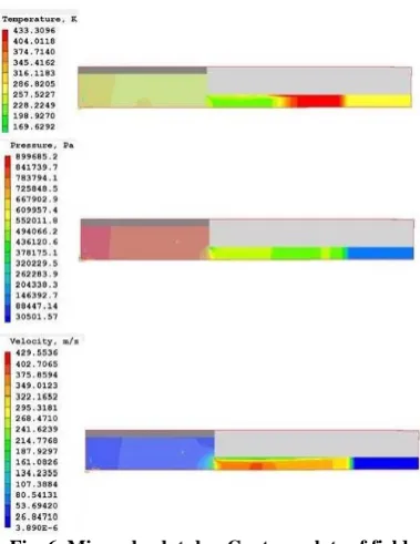
The results for Case 1 produced by PHOENICS some 0.1ms and 0.2ms after rupture of the diaphragm are shown on Fig. 6 and Fig. 7 respectively with corresponding centerline parameter values given on Fig. 8. Velocity profiles showing clearly the boundary layer are given on Fig. 9 at = 0.5. The contour plots are for temperature, pressure and absolute velocity and the normal shock is seen the move to the right through the driven section while the expansion wave is propagating to the left through the driver section. It can be seen that the shock wave gives the driven gas a severe acceleration accompanied by a jump of temperature and pressure.

Fig. 7. Micro shock tube: Contour plots of field variables after 0.2ms.

There is a further increase in temperature and pressure within the driven gas when the shock reaches and is reflected back from the closed end wall. It can be argued that sharper waves and reflections just downstream of the diameter reduction in the driven section by using a turbulence model which produces smaller turbulent viscosities. The 2-layer - turbulence model is known to introduce a smearing effect by producing excessive turbulent viscosities across shock waves and contact discontinuities. Case 1 was also run using the Sarkar et al. (1991) compressibility corrections to the 2-layer - turbulence model which are intended to reduce the predicted turbulence levels due to dilatational effects in high speed flow by this change made no significant change to the calculations.

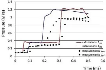
Comparison of the calculated pressure histories with those measured at Andong National University (2016) over a time period of 0.5ms is shown on Fig. 10. The measurements were taken at distances and from the diaphragm location as shown on Fig. 1. The calculated results are broadly in line with the measurements with the shock wave arrival times at both sensor locations for both the initial and reflected shock wave. However there is a significant over-prediction of the pressure level within the driven section of the shock tube. This may be improved by using smaller time steps and/or the incorporation of a second-order time differencing. More likely it is the problem already mentioned of the van Leer MUSCL scheme failing to capture properly the extrema of the shock. As with the Sod calculations (Fig. 3) incorporation of the suggestions of Suresh

and Huynh (1997) may improve matters here. Further work is obviously needed to reduce the over-prediction.

Fig. 8. Micro shock tube: Centreline distribution of variables after 0.1 and 0.2ms.

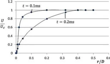
Fig. 9. Micro shock tube: Velocity profiles at

Fig. 10. Micro shock tube: Measured and calculated pressure histories at the sensors

located at and (see Fig. 1).

Two different initial driven pressures were used to study the shock wave propagation as shown in Table 2 (Case 1 and Case 4). The distributions of pressure gradient in front and after the shock wave were calculated using Eq. (15) and are shown on Fig. 11. At the beginning, the pressure gradient has a relatively high value, due to the smaller distance of pressure change across the shock wave. This is followed by much smaller changes in the pressure gradient and the changes may be considered linear. Generally, after the initial period, as the shock wave moves along the driven region, the pressure gradient slowly decreases due to the strength of the shock wave decreasing and the distance of pressure change across the shock wave increasing. When the pressure ratio (Pr) between driver and driven sections is doubled there is a considerable increase in pressure gradient across the shock wave which is maintained over the time period calculated.

Fig. 11. Pressure gradient of the flow in front and after the shock wave for different pressure

ratios.

The Reynolds number values in the region between shock wave and contact surface were obtained at two different pressure ratios as shown on Fig. 12. The density, velocity and dynamic viscosity of the flow changed as the shock wave and contact surface moved along the driven region. The gradual increase in the Reynolds number with time for each of the two cases with is due to the flow velocity increasing in this region. As the initial pressure ratio is increased it can be seen that the Reynolds number decreases accordingly.

Also calculated for Cases 1 and 4 was the scaling parameter S using Eq. (13) as shown on Fig. 13. It

wave travelled through the driven region due to the fact that the distance (the distance between shock wave and contact surface) as used in the scaling parameter became larger with time.

Fig. 12. Reynolds number distributions for different pressure ratios.

Fig. 13. S value distributions for different pressure ratios.

The S values found for the different Pr values follow the same pattern as found for the Reynolds numbers. The effect of incorporating different wall boundary conditions, i.e. slip and no slip conditions, was next examined. It is recognized that because the Knudsen numbers involved were very low there is no real need to use slip as the wall boundary conditions. However it is interesting to examine what difference using slip wall conditions has compared to no slip wall boundary conditions.

The flow slipping near a wall bounded fluid reduces the wall drag effects and thereby increases the shock propagation distance compared to a no slip wall condition. The contact surface under slip conditions shows an opposite trend in its propagation distance, i.e. for a contact surface the slip flow reduces the wave propagation distance compared to the no slip wall conditions. It can be seen from Fig. 14 that the calculated results for Case 1 (No slip) and Case 3 (Slip) follow the foregoing reasoning.

Fig. 14. Shock wave and contact surface locations for slip (Case 3) and no slip (Case 1)

wall conditions over a time period.

Fig. 15. Temperature ratio across the shock wave for slip (Case 3) and no slip (Case 1) wall

conditions over a time period.

The temperature ratio comparisons across the shock front for slip and no slip cases are shown on Fig. 15. The shock strength at any instance is a function of the temperature across the shock front and therefore it can be concluded that the shock strength for the slip case is greater than that for the no slip case. The effect of shock tube diameter is now examined. The simulation with a smaller tube diameter of 3.75mm (Case 2) while keeping the pressure ratio and initial pressure the same as Case 1 shows that the shock strength ( a function of temperature) is reduced in a smaller diameter shock tube. Both Case 1 and Case 2 were calculated with no slip wall conditions and the comparison of the temperature along the centre-line for Case 1 and Case 2 are shown on Fig. 16.

Fig. 16. Temperature distributions for Case 1 and Case 2 along the driven region centre-line at

= .

It is clear that for the smaller shock tube diameter case the temperature rise created by the shock wave

is less when compared to the higher diameter case. This may be explained because the core flow volume bounded by the viscous loss region (i.e. the boundary layer) becomes still smaller and the energy dissipation becomes greater.

The lower temperature rise for Case 2 within the shock wave and therefore the lower shock strength leads to a greater attenuation of the shock wave as the tube diameter decreases. It can be seen from Fig.17 that the shock position for Case 2 is much less with time than Case 1. Both Case 2 and Case 1 shock fronts always lag behind the ideal inviscid analytical solution of Eq. (11) using a theoretical Mach number

M of 2.1.

Fig. 17. Shock location along the driven region centre-line for different tube diameters.

7. C

Numerical calculations have been made to investigate the unsteady flow evolution subjected to various initial conditions and diameters, within a micro shock tube. Reasons for shock attenuation and its dependency on initial pressure ratios, tube diameter and wall boundary conditions have been studied and discussed.

A

The authors appreciate the communications with Dr. Michael Malin of Cham Ltd., Wimbledon, UK, concerning this work, and the sound advice he gave.

R

Andong National University, Unpublished work, (2015).

Arun, K. R. and H. D. Kim (2012a). Computational study of the unsteady flow characteristics of a micro shock tube. Journal of Mechanical Science and Technology 27(2).

Arun, K. R. and H. D. Kim (2012b). Numerical visualization of the unsteady shock wave flow field in micro shock tube. Journal of the Korean Society of Visualisation 10(1), 40-45.

Brouillete, M. (2003). Shock waves at microscales. Shock Waves 13, 3-12.

Daru, V. and C. Tenaud (2009). Numerical simulation of the viscous shock tube problem by using a high resolution monotonicity-preserving scheme. Computer and Fluids 38, 664-676.

Duff, R. E. (1959). Shock tube performance at initial low pressure. Phys. Fluids 2, 207-216. Elhadidy, M. A. (1980). Applications of a

low-Reynolds-number turbulence model and wall functions for steady and unsteady heat-transfer computations. PhD Thesis, University of London, UK.

Godunov, S. K. (1959). A finite-difference method for the numerical computation and discontinuous solutions of the equations of fluid dynamics. Mat. Sb. 47, 271-306.

Karniadakis, G. E. M. and A. Beskok (2002). Micro Flows Fundamentals and Simulation, Springer, New York.

Kohsuke, T., I. Kazuaki and Y. Makoto (2009, January). Numerical investigation on transition of shock induced boundary. 47th _AIAA Aerospace Science Meeting including the New Horizons Forum and Aerospace Exposition, Orlando, Florida.

Mirels, H. (1963). Test time in low pressure shock tube. Phys. Fluids 6, 1201-1214.

Ngomo, D., D. Chaudhuri, A. Chinnayya and A. Hadjadj (2010). Numerical study of shock propagation and attenuation in narrow tubes including friction and heat losses. Computers & Fluids 39, 1711-1721.

Norris, L. H. and W. C. Reynolds (1975) Turbulent channel flow with a moving wavy boundary, Rept. No. FM-10, Stanford University, Mech. Eng. Dept., USA.

Park, J. O., G. W. Kim and H. D. Kim (2014). Experimental study of the shock wave dynamics in micro shock tube. Journal of the Korean Society of Propulsion Engineers 17(5), 54-59.

Rodi W. (1991). Experience with two-layer models

combining the k-e model with a one-equation model near the wall. AIAA-91-0216, 29th Aerospace Sciences Meeting, Reno, Nevada, USA.

Roe, P. L. (1981). Approximate Riemann solvers, parameter vectors, and difference schemes. J. Computational Physics 43, 357-372.

Sarkar, S., G. Erlebacher, M. Y. Hussaini and H. O. Kreiss (1991). The analysis and modelling of dilatational terms in compressible turbulence. J. Fluid Mech. 227, 473-493.

Sod, G. A. (1978). A survey of several finite difference methods for systems of nonlinear hyperbolic conservation. J. Comp. Physics 27, 1-31.

Sturtevant, B. and T. T. Okamura (1969). Dependence of shock tube boundary layers on shock strength. Phys. Fluids 12, 1723-1725. Suresh, A. and H. T. Huynh (1997). Accurate

monotonicity-preserving schemes with Runge-Kutta time stepping. J. Comput. Phys. 136, 83-99.

van Leer, B. (1984). On the relation between the upwind-differencing schemes of Godunov, Engquist-Osher and Roe, SIAM J. Sci. Stat. Comput. 5, 1-20.

Woodward, P. R. and P. Colella (1984). The numerical simulation of two-dimensional fluid flow with strong shocks. J. Comput. Phys. 54, 115-173.

Zeitoun, D. E. and Y. Burtschell (2006). Navier-Stokes computations in micro shock tubes. Shock Waves 15, 241-246.

Zeitoun, D. E., Y. Burtschell and I. A. Graur (2009). Numerical simulation of shock wave propagation in micro channels using continuum and kinetic approaches. Shock Waves 19, 307-316.