A note on digital elevation model smoothing and driving stresses

1

A note on digital elevation model smoothing and driving stresses

Felicity S. McCormack

_{, Jason L. Roberts}

_{, Lenneke M. Jong}

_{, Duncan A. Young}

_{& Lucas H. Beem}

1 _{Institute for Marine and Antarctic Studies, University of Tasmania, Hobart, Tasmania, Australia;}

2 _{Australian Antarctic Division, Kingston, Tasmania, Australia;}

3 _{Antarctic Climate and Ecosystems Cooperative Research Centre, University of Tasmania, Hobart, Tasmania, Australia;}

4 _{Institute for Geophysics, Jackson School of Geosciences, University of Texas at Austin, Austin, TX, USA}

Introduction

Quantifying ice flow is necessary for understanding the dynamics, mass balance and evolution of ice sheets and glaciers. In a steady-state ice sheet or glacier, the net accumulation is equal to the outwards flow distribution, and the ice thickness does not vary in time at any point. The velocity field of the ice when in balance is termed “balance velocity” (Budd & Warner 1996). In the absence of observed velocities, balance velocities have been relied upon for deriving empirical relations for ice flow or sliding properties (e.g., McInnes & Budd 1984), valida-tion of ice-sheet models (e.g., Payne 1999) or fieldwork planning. The calculation of balance velocities requires knowledge of the flow direction, which basic flow theory (Nye 1952, 1957) equates with the direction of steepest surface slope, according to the relation for the gravita-tional driving stress τd:

τd = rgH∇S (1)

where r is ice density, g gravitational acceleration, H ice thickness and S surface elevation. This theory applies

only in regions where surface and bed elevation gradi-ents are small and for horizontal scales of at least the ice thickness (localized features of the surface slope do not affect the flow).

For horizontal scales between 1 and 20 times the ice thickness, longitudinal coupling of longitudinal stress gradients can substantially modify the flow field (Kamb & Echelmeyer 1986). For Eqn. 1 to apply in this instance, thickness and surface slope fields must be smoothed. Kamb & Echelmeyer (1986) demonstrated that an exponential smoothing function appropriately accounts for longitudinal stresses in Eqn. 1. Theory pre-dicts that the horizontal scale of their smoothing func-tion should be between one and three times the ice thickness for temperate valley glaciers and between four and 10 times the ice thickness for ice sheets (although factors such as bed slipperiness can extend these val-ues, e.g., Gudmundsson [2003]). Le Brocq et al. (2006) compared the effect of different smoothing techniques on flux distribution calculations for the West Antarctic Ice Sheet, finding a variety of smoothing scales that pro-duced feasible outcomes. This result suggests the need for an objective means of selecting a smoothing scale Abstract

Ice-flow fields, including the driving stress, provide important information on the current state and evolution of Antarctic and Greenland ice-sheet dynam-ics. However, computation of flow fields from continent-scale DEMs requires the use of smoothing functions and scales, the choice of which can be ad hoc. This study evaluates smoothing functions and scales for robust calculations of driving stress from Antarctic DEMs. Our approach compares a variety of filters and scales for their capacity to minimize the residual between predicted and observed flow direction fields. We find that a spatially varying triangular filter with a width of 8–10 ice thicknesses provides the closest match between the observed and predicted flow direction fields. We use the predicted flow direc-tion fields to highlight artefacts in observed Antarctic velocities, demonstrating that comparison of multiple observational data sets has utility for quality con-trol of continent-scale data sets.

Keywords

Ice-flow direction; smoothing filter; Antarctic ice sheet; ice-sheet dynamics

Correspondence

Felicity S. McCormack, Institute for Marine and Antarctic Studies, University of Tasmania, Hobart, Tasmania 7001, Australia. E-mail: [email protected]

Abbreviations

DEM: digital elevation models; MEaSUREs v2: Making Earth System Data Records for Use in Research Environments, InSAR-Based Antarctica Ice Velocity Map, Version 2, US National Snow and Ice Data Center (Mouginot et al. 2012; Rignot et al. 2011, 2017); RMS: root mean square

that also minimizes some measure of error when calcu-lating the driving stress.

The aim of this study is to determine optimal and sim-ple smoothing functions and scales for continent-wide DEMs of ice-surface elevation for the Antarctic ice sheet. We consider a variety of filters and examine the residu-als between predicted and observed flow direction fields, contrasting the errors associated with using fixed versus spatially varying filter widths. We demonstrate that our technique can facilitate quality control for existing obser-vational data sets of large-scale velocities.

Methods

To determine optimal and simple smoothing functions for continent-wide DEMs, we compared flow directions calculated from smoothed ice-surface DEMs with those of an observed velocity field. Specifically, we considered two ice-surface DEMs: (1) one presented by Bamber et al. (2009), which combines laser altimeter measurements from the ICESat-1 mission with satellite radar altimeter data from the ERS-1 satellite mission; and (2) one devel-oped by Helm et al. (2014), which utilizes data from the CryoSat-2 data acquisition. We used observed surface velocities from the MEaSUREs v2 data set (Rignot et al. 2011, 2017; Mouginot et al. 2012).

We considered three smoothing filters: a Gaussian fil-ter, a triangular filter proposed by Kamb & Echelmeyer (1986) and a bilinear filter. In their analysis of longitudi-nal stresses, Kamb & Echelmeyer (1986) demonstrate that the triangular filter is an accurate alternative to the more computationally costly exponential filter; rather than rep-licate their results, we chose to compare only the triangu-lar filter with the Gaussian and bilinear filters here.

The variable width Gaussian filter is defined by Eqn. 2:

e 1

2 ,

x y

2 2

2 2

2 ω =

πσ

− +

σ ₍₂₎

where full width at half maximum σ is given by a mul-tiple of the ice thickness, H, and the distances from the current point in both x and y directions.

The triangular filter is defined by Eqn. 3:

x y

max 1 , 0.0 , 2 2

ω = +

σ  



 (3)

where again the width σ is scaled by the ice thickness.

The local bilinear surface (z as a function of x and y) is defined as follows:

z x y( , )=a0+a x a y a xy1 + 2 + 3 . (4)

The coefficients a₁ and a₂ are the surface slopes of the DEMs in the x and y directions, respectively, and each of the coefficients a₀–a₃ were chosen to minimize the RMS mismatch between the DEM and the bilinear surface over a moving subwindow centred on the point of interest.

To derive the flow directions from the DEMs, we first applied each of the preceding filters to smooth the DEMs, then calculated the local down-slope directions (q) using the following equation:

atan 2( a2, a1)

θ = − − (5)

Again, a₁ and a₂ in Eqn. 5 are the surface slopes of the DEMs in the x and y directions, respectively. When the local bilinear filter in Eqn. 4 was used, the a₁ and a₂ surface slopes were derived in the same manner as already described; when any of the remaining filters were used, the a₁ and a₂ surface slopes were calculated directly from the filtered DEM. We calculated the uncertainty weighted difference and RMS error between the flow directions predicted from the DEMs, to which each of the filters was applied, and the flow directions of the observed velocity field over the entire ice sheet. We hereafter refer to the difference between the observed and predicted fields as the “bias.” The uncertainties in flow direction for MEaSUREs v2 can be large, for exam-ple, the average absolute error in observed flow directions is 33°. To take into account the impact of flow direction uncer-tainty on the difference statistics, we weighted the bias and RMS error calculations by the uncertainty in the observed flow direction at each point, as follows:

max 0,1 90 .

α − 

  (6)

Here, the total uncertainty (a) was calculated using the error estimates in both the x and y directions from MEa-SUREs v2 and takes values in the range (0,180)°. The resulting scheme in Eqn. 6 assigns zero weighting to all points with uncertainties larger than 90° and a weighting of one to all points with zero associated uncertainty, lin-early weighting between these values. Although the cut-off value of 90° is somewhat arbitrary, uncertainties in flow directions in excess of this threshold are sufficiently large as to warrant exclusion in our comparison between observed and predicted flow fields.

the DEMs, rather than a result of the underlying valida-tion data set.

Because of possible errors in the reference surface velocity directions, we were more concerned with minimizing the weighted RMS error than the bias. We considered two cases for the width of the filter: (1) a spatially invariant filter width, calculating biases for the same range of scaling lengths but with no depen-dence on the ice thickness; and (2) a filter width vary-ing spatially as a function of ice thickness—specifically, directly proportional to ice thickness for a range of smoothing scales.

Results

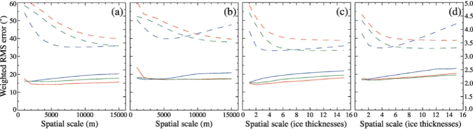
Weighted RMS errors and biases between the predicted and observed flow directions for each of the Bamber et al. (2009) and Helm et al. (2014) DEMs and filters are compared in Fig. 1. RMS errors ranged between 35° and 60°. In all cases, the weighted biases were approximately 2°–3° and positive, irrespective of type of filter, filter width or DEM used.

The patterns in RMS errors and biases calculated using the triangular filter were similar for both DEMs. For a spatially invariant smoothing scale (Fig. 1a, b), the RMS errors monotonically decreased with increasing filter width; for a filter width that varied as function of ice thickness (Fig. 1c, d), the RMS errors decreased rap-idly for smaller spatial scales to an optimal filter width of 8–10 ice thicknesses. The weighted biases showed a slight increase with increasing filter width for both DEMs. The bilinear filter produced similar results to the trian-gular case for each DEM and smoothing scale but with RMS errors on average 0.5° greater. However, the bilin-ear filter came at greater computational expense than the

triangular and Gaussian filters, requiring more than an order of magnitude greater compute time.

The patterns in RMS errors and biases calculated using the Gaussian filter differed markedly from those of the triangular and bilinear filters. For spatially invariant filter widths (Fig. 1a, b), the Gaussian filter RMS errors were minimized for filter widths of 8000–10 000 m with the Bamber et al. (2009) DEM and 4000–6000 m with the Helm et al. (2014) DEM. For Gaussian filter widths that varied as a function of the ice thickness (Fig. 1c, d), the RMS errors were minimized for two to three ice thick-nesses with both DEMs, and the RMS errors increased beyond this width.

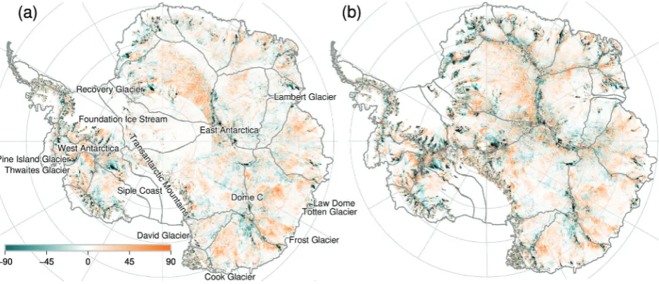
with Roberts et  al.  2011), although these bed features are not necessarily clear from the Bedmap2 bed eleva-tion (Fig. 3; Fretwell et al. 2013). Large absolute weighted biases were associated with both along (azimuth) and across (range) track directions of the satellite swaths incorporated into MEaSUREs v2 (e.g., inland of the Den-man, Frost and Cook glaciers in Wilkes Subglacial Basin; Aurora Subglacial Basin; and Princess Elizabeth Land).

The weighted biases were influenced by two fac-tors: (1) the level of agreement between the predicted

and observed flow directions (Fig. 2b) and (2) the level of uncertainty in the MEaSUREs v2 velocities (Fig. 4). For example, very low absolute biases at latitudes greater than 82.5°S and along drainage divides were a result of large uncertainties in the observed flow direction (Fig. 4), which outweighed large biases between the observed and predicted flow directions in these regions. Large abso-lute weighted biases occurred in regions of poorer sat-ellite coverage, such as in the approach southwards in the range 80°–82.5°S, where there were larger absolute Fig. 3 Bedmap2 bed elevation (m) (Fretwell et al. 2013). Fig. 4 Uncertainties in flow direction (°) calculated from the MEaSUREs v2

dataset (Rignot et al. 2011, 2017).

biases between the observed and predicted flow direc-tions and relatively low uncertainties in the observed flow directions.

Discussion and concluding remarks

Our study examined the impact of filter type and smooth-ing scale on the biases between predicted and observed flow direction fields for the Antarctic continent. We found that Kamb & Echelmeyer’s (1986) triangular fil-ter was most appropriate for minimizing the RMS errors and biases between observed and predicted flow direction fields (Fig. 1), regardless of whether the DEM by Bamber et al. (2009) or by Helm et al. (2014) was used to predict flow direction.

Fixed-width filters produced similar results to filters that varied as a function of ice thickness for each of the filters. For the triangular filter, the RMS errors decreased more rapidly with a varying-size filter. Given minimal increases in both code complexity and computational expense with a varying-size filter, and reduced sensitivity to smoothing scale, we see no benefit in using a fixed-size filter for this application.

Our results suggested that the Kamb & Echelmeyer (1986) triangular filter of 8–10 ice thicknesses and the Gaussian filter of 2–4 ice thicknesses performed sim-ilarly in minimizing the RMS errors. However, in their development of a method to compute balance velocities in ice sheets—which relies on accurate driving stress cal-culations— Brinkerhoff & Johnson (2015) demonstrated that filter widths greater than four ice thicknesses were required to minimize over-convergent flow. Concordant with Kamb & Echelmeyer (1986), the Brinkerhoff  & Johnson (2015) findings suggest that a filter less than four ice thicknesses wide may not be optimal in regions where longitudinal stresses control ice-sheet flow. Apply-ing this to our results suggests that the triangular filter of 8–10 ice thicknesses is optimal for achieving driving stress calculations from DEMs that agree best with veloc-ity observations.

This study has highlighted implications for the calcu-lation of balance velocities from DEMs. Using a triangu-lar filter of width 8–10 thicknesses, we compared biases in observed and predicted flow directions. Weighting the bias by the uncertainties in the observed flow direction allowed us to attribute large biases to the methods used to calculate flow directions and/or the accuracy of the underlying DEMs. Our method assumes that ice flows along the direction of steepest surface slope, which may not necessarily be the case. However, we found large weighted biases towards fast-flowing regions (e.g., Pine Island, Thwaites, Lambert/Fisher/Mellor and Totten

glaciers) where bed topographies were highly chan-nelized, as well as in areas with strong contrasts in bed topography, steep bed slopes or deep topography (<–1000 m). Balance velocities calculated from DEMs using this method may also differ markedly from observed veloc-ities in such regions. This finding has potential conse-quences for applications using balance velocities, for example, mass balance estimates.

Our results also highlighted a potential bias in the observed velocity data. Figure 1 showed a positive bias in predicted flow direction for both the Bamber et al. (2009) and Helm et al. (2014) DEMs when each of the triangu-lar, Gaussian and bilinear filters were used. The bias was slightly lower for the Bamber et al. (2009) data set, which may be a consequence of the Rignot et al. (2017) MEa-SUREs v2 velocities being calibrated against Bamber et al. (2009) rather than Helm et al. (2014). However, Young et al. (2017) compared the Bamber et al. (2009) and Helm et al. (2014) DEMs with the laser altimetry system from the International Collaboration for Exploration of the Cryosphere through Aerogeophysical Profiling II project, finding that the Helm et al. (2014) data set was slightly more accurate than the Bamber et al. (2009) data set at Dome C. Even after weighting the biases by uncertainties in the velocity observations (Fig. 4), large absolute biases between the Helm et al. (2014) DEM and Rignot et al. (2017) were correlated with satellite swaths (Fig. 2), sug-gesting potential artefacts in MEaSUREs v2.

We have determined that a triangular filter with an optimal width of 8–10 ice thicknesses minimizes the residual between observed flow direction fields and those predicted from continent-wide DEMs of ice-sur-face elevation for the Antarctic ice sheet. Such a filter can be used to improve the accuracy of driving stress—and hence balance velocity (Brinkerhoff & Johnson 2015)— calculations by ensuring self-consistent smoothing of continent-wide DEMs. Furthermore, by facilitating the comparison of ice dynamic fields between independent data sets, our technique has applications in identifying potential artefacts in observed fields and may therefore serve as a means for quality control.

Disclosure statement

The authors declare that they have no competing or financial interests.

Funding

Cooperative Research Centres Programme through the Antarctic Climate and Ecosystems Cooperative Research Centre and under the Australian Research Council’s Spe-cial Research Initiative for Antarctic Gateway Partnership (Project ID SR140300001). DY and LB were supported by US National Science Foundation grant PLR-1443690. This is University of Texas Institute for Geophysics (UTIG) contribution #3392.

References

Bamber J., Gomez-Dans J. & Griggs J. 2009. A new 1 km digital elevation model of the Antarctic derived from com-bined satellite radar and laser data—part 1: data and

meth-ods. The Cryosphere 3, 101–111,

Brinkerhoff D. & Johnson J. 2015. A stabilized finite element method for calculating balance velocities in ice sheets.

Geoscientific Model Development 8

Budd W. & Warner R. 1996. A computer scheme for rapid cal-culations of balance–flux distributions. Annals of Glaciology

23

Fretwell P., Pritchard H.D, Vaughan D.G., Bamber J.L., Barrand N.E., Bell R., Bianchi C., Bingham R.G., Blankenship D.D., Casassa G., Catania G., Callens D., Conway H., Cook A.J., Corr H.F.J., Damaske D., Damm V., Ferraccioli F., Forsberg R., Fujita S., Gim Y., Gogineni P., Griggs J.A., Hindmarsh R.C.A., Holmlund P., Holt J.W., Jacobel R.W., Jenkins A., Jokat W., Jordan T., King E.C., Kohler J., Krabill W., Riger-Kusk, M., Langley K.A., Leitchenkov G., Leuschen C., Luy-endyk B.P., Matsuoka, K., Mouginot J., Nitsche F.O., Nogi Y., Nost O.A., Popov S.V., Rignot E., Rippin D.M., Rivera A., Roberts J., Ross N., Siegert M.J., Smith A.M., Steinhage D., Studinger M., Sun B., Tinto B.K., Welch B.C., Wilson D., Young D.A., Xiangbin C. & Zirizzotti A. 2013. Bedmap2: improved ice bed, surface and thickness datasets for

Ant-arctica. The Cryosphere7

Gudmundsson G. 2003. Transmission of basal

vari-ability to a glacier surface. Journal of Geophysical

Research—Solid Earth 108

Helm V., Humbert A. & Miller H. 2014. Elevation and ele-vation change of Greenland and Antarctica derived from

CryoSat-2. The Cryosphere 8

Kamb B. & Echelmeyer K. 1986. Stress-gradient coupling in glacier flow: I. Longitudinal averaging of the influence

of ice thickness and surface slope. Journal of Glaciology32, 267–284, Le Brocq A., Payne A. & Siegert M. 2006. West

Antarc-tic balance calculations: impact of flux-routing algo-rithm, smoothing algorithm and topography. Computers

and Geoscience 32

McInnes B. & Budd W. 1984. A cross-sectional model for

West Antarctica. Annals of Glaciology5, 95–99,

Mouginot J., Scheuchl B. & Rignot E. 2012. Mapping of ice motion in Antarctica using synthetic-aperture radar data. Remote Sensing 4, 2753-2767, https://doi.org/10.3390/ rs4092753.

Nye J. 1952. The mechanics of glacier flow.

Jour-nal of Glaciology 2, 82–93,

Nye J. 1957. The distribution of stress and velocity in glaciers and ice-sheets. Proceedings of the Royal Society of London239, 113–133,

Payne A. 1999. A thermomechanical model of ice flow in

West Antarctica. Climate Dynamics15, 115–125,

Rignot E., Mouginot J. & Scheuchl B. 2011. Ice flow of the

Antarctic ice sheet. Science 333, 1427–1430,

Rignot E., Mouginot J. & Scheuchl B. 2017 - present. MEa-SUREs InSAR-based Antarctica ice velocity map, ver-sion 2.0. NASA Distributed Active Archive Center at the National Snow and Ice Data Center: Boulder, CO. https:// doi.org/10.5067/D7GK8F5J8M8R Accessed on the inter-net at https://nsidc.org/data/nsidc-0484/versions/2 on 20 June 2017.

Roberts J.L., Warner R.C., Young D., Wright A., van Ommen T.D., Blankenship D.D., Siegert M., Young N.W., Tabacco I.E., Forieri A., Passerini A., Zirizzotti A. & Frezzotti M. 2011. Refined broad-scale sub-glacial morphology of Aurora Subglacial Basin, East Antarctica derived by an ice-dynamics-based interpolation scheme. Cryosphere 5, 551–560,

Young D.A, Roberts J.L., Ritz C., Frezzotti M., Quartini E., Cavitte M.G.P., Tozer C.R., Steinhage D., Urbini S., Corr H.F.J., van Ommen T. & Blankenship D.D. 2017. High resolution boundary conditions of an old ice target near

Dome C, Antarctica. The Cryosphere11