Numerical calculation of manoeuvring coefficients for modelling the effect of submarine motion near the surface

(1)

Numerical Calculation of Manoeuvring Coefficients for

Modelling the Effect of Submarine Motion Near the Surface

Christopher David Polis

Bachelor of Engineering in Naval Architecture Graduate Diploma in Business Management

Submitted in fulfilment of the requirements for the degree of

Doctorate in Philosophy

Australian Maritime College

An Institute of the University of Tasmania

(2)

Page ii

This thesis contains no material which has been accepted for a degree or diploma by the University or any other institution, except by way of background information and duly acknowledged in the thesis, and to the best of my

knowledge and belief no material previously published or written by another person except where due acknowledgement is made in the text of the thesis, nor does the thesis contain any material that infringes

copyright.

This thesis may be made available for loan and limited copying and communication in accordance with the Copyright Act 1968.

The publishers of the paper comprising Appendix A hold the copyright for that content, and access to the material should be sought from the respective journals. The remaining non-published content of the thesis may be made available for loan and limited copying and communication in accordance with the Copyright Act 1968.

(3)

Page iii

ABSTRACT

Given the significant amount of time modern submarines conduct operations near the surface of the ocean, there is significant value in the capacity to predict the behaviour of a submarine operating in the near surface region. During most near surface operations, the primary forces involved are due to transient ocean waves and are statistical in nature. Yet there is also a contribution from the motion of the submarine near the surface, which has received less attention from researchers. The aim of this thesis is to determine the nature of the changes that occur in the manoeuvring forces acting on a submarine due to its own motion when operating near the ocean surface. Currently, coefficient-based manoeuvring models are utilised to predict deeply submerged submarine motion. However, research has shown that these coefficients change when near the surface due to the proximity and form of that surface.

Utilising numerical computation with validation against experimental results, the sources of coefficient variation from their deeply submerged values in the near surface region are identified. The parameters that this variation depends upon are assessed, and the coefficients of motion that vary as a result are identified.

Two novel methodologies based upon the use of numerical planar motion are proposed by which the variation found in the near surface region can be measured across the operating envelope and the changes found for a standard submarine form are thus determined.

The results of these tests show that, of the coefficients assessed, those that have the most significant impact upon submarine motions in the near surface region are:

• Coefficient of normal force as a function of square of the axial velocity; • Coefficient of normal force as a function of velocity in the z-axis;

• Coefficient of normal force as a function of acceleration in the z-axis; and • Coefficient of pitch moment as a function of velocity in the z-axis.

Note: the z-axis is vertical in the submarine’s frame of reference.

It was also found that the amplitude of a numerical planar motion can be reduced to a minor fraction of a submarine’s diameter without loss of accuracy. More

significantly, motions of such scale were found to render the coefficients

approximately constant over the period of oscillation. This allows the utilisation of this method for the numerical estimate of linear acceleration and velocity coefficients in the near surface region, which are not obtainable via conventional methods. The ability to estimate these coefficients — along with those obtainable through extending these methods to simulating pure pitch — will enable substantially

(4)

Page iv

Page v

4.7 Pitch Moment due to Constant Depth Motion at an Angle of Trim ... 61

4.8 Heave Force due to Level Motion at an Angle of Trim, at Various Froude Number .. 64

4.9 Summary ... 68

5. VALIDATION OF HORIZONTAL PLANAR MOTION ... 70

5.1 Objectives and Methodology ... 70

5.2 Theory ... 70

5.3 Reference Physical Model Test Data ... 71

5.4 CFD Modelling ... 71

5.5 Results ... 73

5.6 Summary ... 74

6. PLANAR MOTION METHODS FOR ANALYSIS NEAR A FREE SURFACE ... 75

6.1 Objectives and Methodology ... 75

6.2 Fractional Planar Motion ... 76

6.3 Sudden Linear Acceleration ... 85

6.4 Variation in coefficients ( ′, ′, ′ and ′ ) with depth ... 91

6.5 Summary ... 94

7. CONCLUSIONS AND RECOMMENDATIONS ... 96

7.1 Concluding Remarks ... 96

7.2 Recommendations for Future Work ... 98

7.3 Final Statement ... 98

BIBLIOGRAPHY ... 99

Appendix A - Enabling the Prediction of Manoeuvring Characteristics of a Submarine Operating Near the Free Surface ... 104

Appendix B - Prediction of the hydroplane angles required Due to High Speed Submarine Operations near the Surface ... 116

(6)

Page vi

ACKNOWLEDGEMENTS

There are a number of people who I cannot thank enough for their contributions to the work required to complete this project.

Thank you to Professor Dev Ranmuthugala: for your persistence with me over these years. I appreciate the insight that you bring to such a broad range of topics, and your capacity to illuminate significant issues that I may have otherwise passed up as minor. Without you, this never would have started, and never would have been completed.

Thank you to Dr Jonathan Duffy: for your ongoing encouragement, presence and discipline; you kept me going through some tough periods. Thank you for sharing your expertise, and much of your own experience. It was very much appreciated. Thank you to Professor Martin Renilson: for the deep understanding you presented me with of the topic and tasks set before me. For taking the time to see me, whether near or far, through the midst of what hasn’t been the easiest of times for you. It was an honour.

Thank you to Charl Fourie: for granting me an understanding of myself that I lacked, and the tools and structures required to mitigate the limitations within myself. Thank you to Alex and Esther Ashworth-Briggs, Allan Belle, Zhi Leong, Max Haase, Howan Kim and many others at the AMC Research Hub. Thank you for journeying with me, and for the countless contributions and exhortations you made that enabled me to complete this thesis.

Thank you to Luciano Mason, who was always right there, and always right.

Thank you to my son, Benjamin, who shared the research experience with me on our many ‘university days’, and sat with me over many evenings towards the end,

keeping me focussed on the task at hand.

And finally, thank you to my wife Natalie, who has stood by me through the hard times, and celebrated with me in the good times. The seemingly never ending process does have an end, and your love and commitment to me has allowed me to reach it. I am yours, alone, always.

To each and every one of you: May God bless you and keep you. May you be granted life in its fullness and joy in the years to come.

Yours humbly,

(7)

Page vii

NOMENCLATURE AND CONVENTIONS

Directional Conventions

Linear and rotational axis system

X,Y,Z Earth fixed axes x,y,z Body fixed axes

, Velocity, acceleration along the x axis , Velocity, acceleration along the y axis , Velocity, acceleration along the z axis , Roll rate, acceleration

, Pitch rate, acceleration , Yaw rate, acceleration

Angle of Roll Angle of Pitch Angle of Yaw

Nomenclature

Buoyancy Force Uniform velocity of flow Centripetal-Coriolis Matrix

Model to Full Scale Thrust Coefficient Linear Resistance Coefficient

(8)

Page viii

Depth of doublet submergence

Force due to Resistance and Propulsion characteristics Acceleration due to gravity

( ) Gravity vector

Depth from static free surface to the submarine hull centreline in metres ⋆ _{Non-dimensionalised depth, H/D}

Moment of Inertia about y-axis Decay constant

Length of submarine hull in metres Dummy integration variable Doublet Strength

Mass Matrix Moment about y-axis

⋆ _{Function of}_{Pitch Moment across all values of}

Coefficient of Pitch Moment as a function of Coefficient of Pitch Moment as a function of ⋆ _{Function of}_{Pitch Moment across all values of} ⋆ _{Function of}_{Pitch Moment across all values of}

Coefficient of Pitch Moment as a function of Coefficient of Pitch Moment as a function of | | Coefficient of Pitch Moment as a function of | |

Coefficient of Pitch Moment as a function of | | Coefficient of Pitch Moment as a function of | | ⋆ Coefficient of Pitch Moment as a function of

Coefficient of Pitch Moment as a function of Coefficient of Pitch Moment as a function of Correction to as a function of Command Ratio

Moment about the z-axis

(9)

Page ix

Coefficient of Yawing Moment as a function of Pressure

Radius

, Strength of Momentum source in the y-axis direction , Strength of Momentum source in the z-axis direction

Time

Change in Time Total velocity

Linear velocity of origin of body axes relative to fluid Velocity component in y-axis direction

Velocity component in z-axis direction Instantaneous Velocity Component Mean Flow Component ′ Time Variant Flow Component

Instantaneous Velocity Component Command Velocity

Friction Velocity Gravitational Weight

x-axis Distance from centre of rotation to centre of buoyancy x-axis Distance from centre of rotation to centre of gravity Flow component axis

Flow component axis Axial Force

⋆ Coefficient of Axial Force as a function of ⋆ _{Function of}_{Axial force across all values of}

Coefficient of Axial Force as a function of ⋆ _{Function of}_{Axial force across all values of}

Coefficient of Axial Force as a function of Coefficient of Axial Force as a function of ⋆ _{Function of}_{Axial force across all values of}

(10)

Page x

Coefficient of Axial Force as a function of Coefficient of Axial Force as a function of Coefficient of Axial Force as a function of Coefficient of Axial Force as a function of Lateral Force

Coefficient of Lateral Force as a function of Coefficient of Lateral Force as a function of | | Coefficient of Lateral Force as a function of | |

Δ Distance from wall

Non-dimensionalised Distance from Wall

z-axis Distance from centre of rotation to centre of buoyancy z-axis Distance from centre of rotation to centre of gravity Normal Force

⋆ _{Function of}_{Normal force across all values of}

Coefficient of Axial Force as a function of Coefficient of Axial Force as a function of Coefficient of Axial Force as a function of ⋆ _{Function of}_{Normal force across all values of}

⋆ Coefficient of Axial Force as a function of ⋆ _{Function of}_{Normal force across all values of}

Coefficient of Axial Force as a function of Coefficient of Axial Force as a function of | | Coefficient of Axial Force as a function of | |

Coefficient of Axial Force as a function of | | Coefficient of Axial Force as a function of | |

Normal force due to stern plane angle Normal force due to bow plane angle

Acceleration correction for Normal force due to stern plane , , Coefficients for variation in drag due to command speed

(11)

Page xi

Earth fixed position / orientation vector Ratio of command velocity to velocity

/

Dynamic Viscosity Kinematic Viscosity Wave speed Control Vector

x-axis force component of Control Vector y-axis force component of Control Vector z-axis force component of Control Vector

Roll moment component of Control Vector Pitch moment component of Control Vector Yaw moment component of Control Vector

(12)

Page xii

Non-Dimensionalisation

C

OEFFICIENTS

= 1 2

⋆=₁ ⋆

2 = 1 2 = 1 2 = 1 2 = 1 2 | |= | | 1 2 = 1 2 | |= | | 1 2 | | = | | 1 2 = 1 2 = 1 2 = 1 2 = 1 2 = 1 2 = 1 2

⋆=₁ ⋆

2 = 1 2 = 1 2 = 1 2 = 1 2 = 1 2 = 1 2 = 1 2 = 1 2

⋆ =₁ ⋆

2 = 1 2 = 1 2 | |= | | 1 2 = 1 2

⋆=₁ ⋆

2 = 1 2 | |= | | 1 2 = 1 2

| |=₁ | |

(13)

Page 1

V

ELOCITIES

= ; = ; = ; = ; = ; =

A

CCELERATIONS

= ; = ; = ; = ; = ; =

D

ISTANCES

⋆ _{= ;} ⋆ ₌

=

A

NGULAR

V

ELOCITIES

=

S

PEED

-L

ENGTH

R

ATIOS

(14)

Page 2

ABBREVIATIONS

AMC Australian Maritime College

AMCTT Australian Maritime College Towing Tank

AUV Autonomous Underwater Vehicle

BSL Baseline

BSL-RSM Baseline – Reynolds Stress Model

CFD Computational Fluid Dynamics

DNS Direct Navier Stokes

DTMB David Taylor Model Basin

EARSM Explicit Algebraic Reynolds Stress Model

EFD Experimental Fluid Dynamics

FPM Fractional Planar Motion

HPMM Horizontal Planar Motion Mechanism

LCG Longitudinal Centre of Gravity

PMM Planar Motion Mechanism

RANS Reynolds Averaged Navier-Stokes

RSM Reynolds Stress Model

SLA Sudden Linear Acceleration

SNAME Society of Naval Architects and Marine Engineers

SST Shear Stress Transport

UTAS University of Tasmania

VOF Volume of Fluids

VPMM Vertical Planar Motion Mechanism

The following capitalised terms are used but are formal names, not abbreviations. ANSYS

(15)

Page 3

LIST OF FIGURES AND TABLES

Figure 1-1 Changes in Australian Submarine Designs over Time ... 1

Figure 2-1 Pitch and Normal Force Coefficients as a function of Pitch Angle ... 10

Figure 3-1 Linear and Rotational Axis System ... 14

Figure 3-2 X' as a function of angle ... 17

Figure 3-3 M' as a function of angle ... 17

Figure 3-4 Resistance as a function of Froude Length Number, Model 1257 ... 20

Figure 3-5 Resistance as a function of Froude Length Number, Model 1242 ... 20

Figure 3-6 Lift Coefficient as a function of Froude Number and Submergence ... 21

Figure 3-7 Pitch Coefficient as a function of Froude Number and Submergence ... 21

Figure 4-1 Series 2 Cases ... 28

Figure 4-2 Identical mesh shown with water surface (left) and without (right) ... 29

Figure 4-3 SUBOFF Profile Calculated from Groves (1989) ... 29

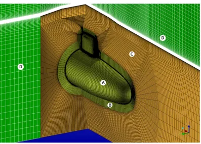
Figure 4-4 SUBOFF Model shown in Symmetric Domain ... 30

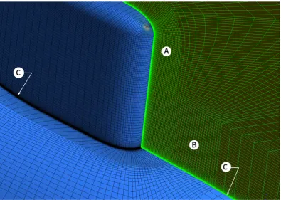
Figure 4-5 Near Hull Blocking Arrangement on Symmetry Plane ... 30

Figure 4-6 3D Sectional View of SUBOFF Meshing. ... 31

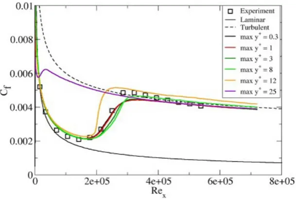
Figure 4-7 Subdivision of Turbulent Boundary Layer ... 32

Figure 4-8 Law of the Wall ... 33

Figure 4-9 Variation of Skin Friction (Cf) on a flat plate with +... 33

Figure 4-10 Boundary Layer Meshing ... 34

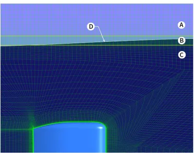
Figure 4-11 Free Surface Mesh Layering ... 35

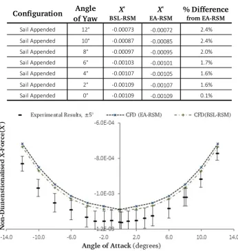
Figure 4-12 Axial Force at Different Angles of Yaw, SUBOFF with Sail ... 38

Figure 4-13 Y-Force at Different Angles of Attack, SUBOFF with Sail... 39

Figure 4-14 Unstable Small Amplitude Surface Waves Traversing Wave Train. ... 41

Figure 4-15 Axial Force as a function of Mesh Density ... 42

Figure 4-16 Effect of Mesh Density on Wave Height. ... 43

Figure 4-17 Detail of First Wave Trough at Different Mesh Densities, ... 44

Figure 4-18 DTRC Equipment Arrangement ... 45

Figure 4-19 Sting Supported SUBOFF as used in the AMC Towing Tank ... 46

Figure 4-20 Comparison of CFD and Experimental Data for SUBOFF Model ... 46

Figure 4-21 Details of DTRC Support Posts ... 47

Figure 4-22 Modelled DTRC Supports ... 47

Figure 4-23 Mesh Arrangement on SUBOFF Surface around Posts ... 48

Figure 4-24 Variation in Drag with Angle of Attack, With and Without Supports ... 49

Figure 4-25 Variation in Drag with Angle of Attack, With and Without Supports ... 49

Figure 4-26 Axial Force Coefficient as a function of at H* 1.8, 2.2, 2.5, 2.8 ... 51

Figure 4-27 Axial Force Coefficient as a function of ⋆ at 0.400, 0.421, 0.444, 0.471 ... 51

Figure 4-28 Normal Force Coefficient as a function of at H* 1.8, 2.2, 2.5, 2.8 ... 52

Figure 4-29 Normal Force Coefficient as a function of ⋆ at 0.400, 0.471 ... 52

Figure 4-30 Pitch Moment Coefficient as a function of at ⋆ 1.8, 2.2, 2.5, 2.8 ... 53

Figure 4-31 Pitch Moment Coefficient as a function of ⋆ at 0.400, 0.421, 0.444, 0.471 ... 53

Figure 4-32 Experimental Variation in Axial Force (Neulist 2011) ... 54

Figure 4-33 Variation in Axial force with trim, for SUBOFF with sail appended at 0.422 ... 56

Figure 4-34 SUBOFF w/ Sail, Non-dimensionalised Axial force as a function of Trim at 0.422 ... 57

Figure 4-35 SUBOFF w/ Sail at Level Trim, ’⋆ as a function of and ⋆ ... 58

Figure 4-36 SUBOFF w/ Sail, ’ as a function of and ⋆ ... 59

Figure 4-37 SUBOFF w/ Sail, ’ as a function of and ⋆ ... 60

Figure 4-38 Pitch Moment as a function of Angle of Trim, 0.422 ... 61

(16)

Page 4

Figure 4-40 SUBOFF w/ Sail, as a function of and ⋆ ... 63

Figure 4-41 SUBOFF w/ Sail, _{| |}as a function of and ⋆ ... 63

Figure 4-42 SUBOFF w/ Sail, as a function of and ⋆ ... 64

Figure 4-43 ′ as a function of Trim Angle, 0.422 Fitted to Equation 4.33 ... 65

Figure 4-44 ′ as a function of Trim Angle, 0.422 Fitted to Equation 4.34 ... 65

Figure 4-45 SUBOFF w/ Sail, _⋆ as a function of _⋆ and ... 66

Figure 4-46 SUBOFF w/ Sail, as a function of ⋆ and ... 66

Figure 4-47 SUBOFF w/ Sail, _{| |}as a function of _⋆ and ... 67

Figure 4-48 SUBOFF w/ Sail, as a function of _⋆ and ... 67

Figure 5-1 Mesh Cross-section showing Simplification of Existing Mesh (Half Mesh Shown) ... 72

Figure 5-2 Decay in Time Domain Solution Stability with Decreasing Timestep ... 73

Figure 6-1 Z-Coefficients as a function of Amplitude, Deeply Submerged ... 77

Figure 6-2 Pitch Moment Coefficients as a function of Amplitude, Deeply Submerged ... 78

Figure 6-3 Normal Force Coefficients as a function of Frequency, Deeply Submerged ... 79

Figure 6-4 Pitch Moment Coefficients as a function of Frequency, Deeply Submerged ... 79

Figure 6-5 Normal Force Coefficients as a function of Amplitude, Near Surface ... 81

Figure 6-6 Pitch Moment Coefficients as a function of Amplitude, Near Surface ... 82

Figure 6-7 Wave Profile at Different Amplitudes of Oscillation ... 82

Figure 6-8 Wave Profile Offset at different Amplitudes of Oscillation ... 83

Figure 6-9 Effect of Oscillation Frequency on Normal Force Coefficients Near the Surface ... 84

Figure 6-10 Effect of Oscillation Frequency on Pitch Moment Coefficients Near the Surface ... 84

Figure 6-11 Typical Normal Force after a Sudden Change in Acceleration (First 20 timesteps) ... 85

Figure 6-12 Response of Normal Force to Sudden Acceleration, After Initial Oscillation ... 87

Figure 6-13 Typical Pitch Moment after Sudden Change in Acceleration (First 20 timesteps) ... 87

Figure 6-14 Force Coefficient as a function of Time at Different Accelerations ... 88

Figure 6-15 Pitch Coefficient as a function of Time at Different Accelerations ... 88

Figure 6-16 Response to Sudden Acceleration, Different Directions ... 89

Figure 6-17 Absolute Response to Sudden Acceleration, Different Directions ... 90

Figure 6-18 Coefficients of Normal Force as a function of Submergence ... 92

(17)

Page 5

1. INTRODUCTION

1.1 Background

The relationship that submarines have with the surface of the water has evolved in a fascinating arc over the last 140 years. In the last thirty years of the 1800’s, submarines progressed from being mere curios to promising but untried platforms. In World War 1, submarines — then vessels that primarily operated surfaced but with the capacity to submerge — showed significant naval value through their distinct capabilities. Early in World War 2, most retained a significant surfaced

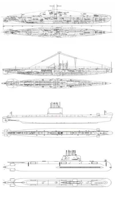
warfighting capability, including the possession of deck mounted guns. But by the end of the War, submarine designs had evolved to focus on underwater performance and capability. Figure 1-1 shows the evolution of Australian submarines over the last 100 years.

However, the most substantial changes were yet to come, with the development over the next two decades of low drag underwater forms, and critically the development of nuclear propulsion. These advances moved the submarines preferred operating depth well below of the surface, eliminating most of the ties that made operating near the surface necessary.

Yet even today, near surface operations remain a significant consideration in the design and operation of submarines. A significant proportion of modern submarine operations require operation in the near surface region. Conventional diesel-powered submarines (SSK) such as those used in Australia spend a considerable portion of time near the surface in order to recharge batteries, and most submarines conduct operations that require access to the surface such as surveillance, communication and warfare (Joubert, 2006). There has been an arc of design and research focus that has progressed from first developing the capacity to move under the surface, then to optimise this capacity, and a renewed focus on the capacity to operate effectively, stealthily and safely in the water just beneath the surface where so many of the critical operations of a submarine take place.

[image:17.595.325.535.81.429.2]

Over this time, an immense amount of research has gone into developing ways to assess and predict the dynamic capabilities of a submarine in the design phase. The first mathematical models of the submarine in the near surface environment were

Figure 1-1 Changes in Australian Submarine Designs over Time

(18)

Page 6

developed in the 1920’s, developed further through the testing of physical models in the 1930’s as nations prepared for a renewed outbreak of war (Weinblum et al, 1936). Primarily in these early periods, testing was focussed on the resistance of the models. In the post-war period efforts moved to the development of various means of assessing the manoeuvrability of a submarine using physical scale models in captive tests. By the 1960’s, the nature of submarine manoeuvring was captured in six degree mathematical models of motion (Gertler & Hagen, 1967) utilising tests that isolated the response of a submarine to specific changes in its operational condition. In the period since then, improvements in model testing have continued, with the development of models capable of self-propulsion and the systems required to accurately capture the actions and motions of the model in that state. Yet such testing remains expensive, requiring large and complex models, controlled facilities, and significant staffing. In the same period, there has also been a rapid rise in the development of Computational Fluid Dynamics (CFD), and the computational power required to effectively utilise it. This offers the potential of not only lower costs, but also of reduced timeframes and greater opportunity to explore different design options. Furthermore, CFD offers the capacity to model in detail the complex flows around the submarine and its appendages. This has offered insight into the basic fluid dynamic processes at work that were difficult to obtain experimentally. Despite these advances, it remains the case that both scale model and computational efforts must be able to be correlated to full scale results.

1.2 Problem Definition

Given the focus modern diesel-powered submarines have on operations in the near surface environment, there has been an understandable move towards research on the design of submarines specifically for this environment (Joubert, 2006). Their distinct differences from nuclear powered submarines — i.e. their need for air, finite range, reduced speed and lower cost — all skew the operational profile in practice. Blue water fleet support is of reduced significance — though not blue water fleet deterrence (Kopp, 2012) — and operation within the more complex environments of littoral waters and near the ocean surface is demanded. The capacity to reflect these changes in mission within the design process to achieve greater effectiveness in role performance is highly desirable.

In order to conduct a design optimisation focussing on operations in this space, the impact of operation near boundaries must be able to be estimated based upon the submarine’s geometry. While these boundaries include the seabed and other large scale structures, and even discrete shifts in water density that occur as a submarine changes from one layer of water to another, the primary boundary of influence is the ocean surface. The additional effects that result from operating near the water

(19)

Page 7

2013). Underlying this is a self-generated load derived from the motion of the submarine itself (Griffin, 2002), and at higher Froude Number this component increases in significance.

The estimation of the additional loads that occur in the near surface region is a complex matter. The creation and testing of self-propelled, scaled physical models are expensive and time consuming, but provides a level of accuracy that other methods have not yet delivered (Leong, Ranmuthugala, Penesis & Nguyen, 2012). Simpler physical models can be utilised in controlled testing to derive characteristics of motion for use in a mathematical model of submarine motion. The other

methodology that is available and utilised today is the modelling of flows utilising CFD. Although CFD can be utilised to directly model the response in the near surface environment of full scale submarines in operation, this remains compute-resource intensive. Utilising CFD in a similar fashion to captive model testing to model a number of programmed conditions in order to determine the characteristics of

motion opens up the possibility of relatively quickly and cheaply assessing a far wider range of design options, although costs and time can escalate.

In order to be able to model operations in the near surface environment, such that a wide variety of options may be considered without excessive demand on economic or computation resources, two basic components of research are required.

• CFD based predictions that produce outcomes within a validated error band.

• A mathematical model of submarine motion that accounts for the difference in behaviour between the well-studied deeply submerged environment and the near surface environment.

1.3 Research Question

The resolution of the entire problem outlined above is well beyond the scope of a single PhD study. However, in order to contribute to this, the thesis that follows seeks to resolve the following question:

What changes occur in the manoeuvring forces acting on a submarine due to its own motion when operating near the ocean surface compared to operating deeply submerged?

1.4 Research Objectives

In order to establish validated answers to the above question, a program of study and original research were undertaken. This program first set out to establish what is already known regarding the changes in manoeuvring coefficients near the ocean surface, and then to fill in the gaps in knowledge through research.

To do so requires the achievement of a number of specific objectives:

(20)

Page 8

• Determine which existing coefficients of motion vary significantly in the near surface environment and how the extent and nature of this variation can be modelled. Identify the parameters that this variation depends upon.

• Ascertain whether additional coefficients need to be included in the manoeuvring model to capture the motion response of a submarine in the near surface environment.

• Propose methodology by which the variation may be estimated through the simulation of planar motion tests in the near surface region, and how these results can be encoded into modified and/or additional coefficients.

1.5 Methodology

The following methodology has been utilised:

• A literature review was conducted into existing research on mathematical models of submarine motion, testing methodology, physical and model testing and numerical simulation conducted in the near surface region. • The sensitivity of existing models to the various coefficients therein was

examined in order to give insight into which of those coefficients were most significant in the modelling of submarine motion, and thus sensitive to change imposed by operation within the near surface region.

• A generic submarine form was be modelled undergoing standard testing manoeuvres, adapted as necessary to suit the near surface region. This was undertaken using CFD, validated against existing numerical and experimental test data, and utilised to assess the response associated with operating near the ocean surface.

• A preliminary investigation into the variation of the primary forces that occur in straight level motion as the submarine approaches a free surface was conducted. A more systematic mesh verification and validation was then undertaken for conditions both deep & near the surface. It

considered both bare hull and sail appended configurations, with and without experimental apparatus attachments, for comparison against experimental data identified during the literature review.

• Research was then conducted into the effects of attitude variation of the submarine near the free surface, at a range of depths and Froude

Numbers.

(21)

Page 9

capacity for determining hydrodynamic characteristics. This study was inferentially validated through validation against physical model testing in both the deeply submerged and near surface conditions.

• A study of small motions under instantaneous, constant acceleration (Sudden Linear Acceleration) was also conducted with the intent to derive acceleration coefficients in the near surface region. These results were compared with those obtained using Fractional Planar Motion.

• Finally, utilising these results, the significance of various coefficients to modelling operation near the free surface was assessed by evaluating the change that occurred in the coefficient near the free surface and the sensitivity of the model to change in that coefficient. The coefficients were then grouped into bands of significance on the basis of the expected effect of their near surface changes on the manoeuvring model.

1.5.1 Research Outcomes and Novel Contributions

The research outcomes of this work are summarised as follows:

• CFD based modelling of near surface test operations to determine relevant coefficients of motion in the vertical plane, including original work

considering the effect of trim in the near surface region;

• Development of both Fractional Planar Motion and Sudden Linear Acceleration as means by which coefficients of acceleration can be determined in the near surface region.

• Assessment of a range of coefficients dependent upon motion in the z-axis for their significance in the modelling of the near surface motion of submarines.

1.6 Arrangement of this Thesis

Following this brief introduction, the remainder of this thesis is structured as follows: • Chapter 2 contains a literature review, discussing the body of research

underlying this thesis. The study of waves and the influence of bodies moving under them; the development of the coefficient based

manoeuvring model; experimental and computational techniques are recounted, leading to the capability to develop this thesis.

• Chapter 3 discusses the theory and mathematical concepts underlying the modelling of submarine behaviour near the free surface. This includes the coefficient based manoeuvring model; its sensitivity to the changes in various coefficients; existing studies and calculations of the effect of the free surface on the model and its coefficients; choice of a deeply

(22)

Page 10

• Chapter 4 presents the verification and validation process underlying the CFD simulation conducted throughout this thesis. It then presents a study describing the relationship between depth, submergence, Froude Length Number, and the additional response observed in the vertical plane to steady state operation parallel to the free surface. This is then extended with a second study regarding the variation of these forces with changes in trim to the surface which assesses the significance of the coefficients based upon velocity in the x and z-axis for significance. However, these studies, given their steady state nature were unable to determine any change in the acceleration coefficients.

• Chapter 5 details the numerical modelling of pure sway in the deeply submerged regions and its validation against published data. This was a functional but a necessary step, providing a degree of assurity of process to obtaining the remaining coefficients in Chapter 6.

• Chapter 6 discusses the conceptual rationale and evaluation of both Fractional Planar Motion (FPM) and Sudden Linear Acceleration (SLA) efforts to develop a test methodology suitable for deriving acceleration based near surface manoeuvring coefficients. This is followed by the selection and use of FPM to provide a numerical estimate of the resultant coefficients at a series of depths.

• Chapter 7 summarises the conclusions resulting from this work and provides recommendations from the findings and for future work.

(23)

Page 11

2. LITERATURE REVIEW

2.1 Historic Origins

The development of the theory of water waves (Craik, 2004 and 2005) has been touched by the work of some of the greatest scientific minds of the last 400 years: Newton (1687), Euler (1761), Laplace (1776), Poisson (1818), Cauchy (1827), Stokes (1847), Kelvin (1887), Michell (1893). Yet it was really only in the 20th

century that work began in earnest on the understanding of the waves made by moving objects near the free surface, and only in the second half of that century that attention was truly brought to bear upon the manoeuvring of submarines, driven by the changing needs of modern navies.

The waves generated on the ocean surface by the passage of a submarine underneath are not simply a function of submergence and Froude Length Number, but also the form and current attitude of the submarine to that surface, along with the time history of those characteristics (Havelock 1950). At each point in time, energy is added to the surface wave system by the submarine in a manner dependant on the conditions of the submarine at that point. This energy is largely retained in the surface through the generation of waves, which travel away from the point of

generation at a fixed speed. The integration of this continuous function of generation and travel of waves determines the effect of the nearby submarine on the water surface, and vice versa.

2.2 Coefficient Based Manoeuvring Models

The initial expression of the motion of a rigid body in a fluid — the first hydrodynamic models — were developed independently by Thompson & Tait (1867), Kirchhoff (1869) and Kelvin (1871). In these, the equations were developed as components of the impulse, obtained as the gradients of the energy relative to the components of motion. Lamb (1916 and 1932) refined the expression of these models and collated developments in the field into his Hydrodynamics text.

In 1946 Abkowitz prompted the development of a standard set of notation across the field, which was formalised through a series of committees into the notation that is still utilised today (SNAME, 1952). Abkowitz later wrote a summary text on stability and motion control, focussing on the derivation and evaluation of manoeuvring coefficients and models (Abkowitz, 1969).

(24)

Page 12

Tuck, 1964); Flat Ship Theory (MacCamy, 1964); and Strip Theory (Vassilopoulos & Mandel, 1964).

A number of sets of standardised equations for modelling the motion of a submarine in deep water were developed. Early formulations like those produced by the Society of Naval Architects and Marine Engineers (SNAME, 1952) were built upon by the David Taylor Model Basin (DTMB), resulting in a standardised form published as Standard Equations of Motion for Submarine Simulation (Gertler & Hagen, 1967). This set of equations, with modifications to suit the data gathered and the

arrangement of the particular submarine or submersible is still utilised today, however refinement of this general form continued (Feldman, 1979).

Working from this basis, the general equations are commonly either simplified or modified to suit a particular vessel (Healey & Lienhard, 1993; Prestrero, 2001). Other modifications are made based upon a preference for using alternate

formulations for the non-linear components (Clarke, 2003) rather than the modulus quadratic form adopted to account for non-linearity in Gertler & Hagen (1967). There has also been a move to expressing the equations in vector notation (Fossen, 1994) which has allowed a more compact form of notation.

2.3 Near Surface Hydrodynamics

The theory of waves produced by submerged objects commenced in earnest with the work of Lamb (1913). Initially offering a reprise of the formulation employed by Cauchy (1827) nearly a century earlier, stating the stream function describing two-dimensional flow, Lamb then went on to develop a boundary condition for the free surface and derive a general solution. From this point, by supposing an oscillating source some distance below the surface, Lamb developed an expression for the response due to an infinite cylinder of small radius oscillating near the surface. He then further developed this to the surface response due to an infinite cylinder transverse to a constant flow and calculated the resulting wave resistance.

Havelock (1917a) reproduced the same problem by an alternate method considering the pressure on the cylinder surface, before extending the work further (Havelock, 1917b) to consider the resistance of a submerged sphere in the flow.

Havelock (1919) subsequently repeated this result with a simpler if less direct method whereby the resistance was calculated by evaluating the moving pressure field required to form the same wave pattern. Lamb (1926) built upon this to provide an integral for determining the resistance of an arbitrarily shaped body moving below a free surface.

(25)

Page 13

Havelock continued his studies and development of this theory across the following decades, leading to works in the 1950’s considering the flow resulting from a specified body following a specified path at a specified speed.

Havelock’s body of work was later developed further by Tuck (1971 and 1987) and Lazauskas (2005) to deal with complex forms utilising numerical methods. Tuck, building on the thin-ship theory of Michell (1898), allowed any zx-plane symmetrical hull form to be represented by a source plane of strength determined by the hull demi-beam at each point.

A number of alternate approaches have also been developed, applying different numerical methods to the problem of modelling the manoeuvring of a submarine that are potentially applicable in the near surface. Some approaches, such as that employed in Jensen, Chislet & Romeling (1993) and Eloot & Vantorre (2003) replace the practice of utilising one or more fixed manoeuvring coefficients that serve to approximate a nonlinear curve with a tabulated and interpolated response across the range tested. Others such as Nahon (1996) utilise alternate formulations where established empirical formulae for the different responses are utilised instead of coefficients of form. Typically, these methods exchange a requirement for additional data and/or calculation for the ability to follow a response that departs from the coefficient-based estimate.

2.4 Experimental Methods

Alongside the theoretical development that was occurring throughout this period, the capacity to carry out physical model experiments to ascertain the response of the submarine also developed over this period. One of the earliest formal studies of the wave resistance of submarines was conducted by Weinblum, Amtsberg &

Bock (1936) in Germany. This work compared the theoretical models of the day against a series of model tests of bodies of revolution, leading to a series of resistance curves showing wave resistance at various Froude Numbers.

After the Second World War, a substantial program of experimental and developmental works was carried out, developing methods for deriving the

hydrodynamic characteristics of submarines, not only in terms of their drag (either submerged or near the surface), but also the manoeuvring characteristics.

The techniques and equipment developed included the Rotating Arm (Brownell, 1956) and Planar Motion Mechanism (Gertler, 1967). In addition to oblique tow tests conducted with the vessel in a normal towing tank, these tests sufficed to provide the primary coefficients for both velocity ( , , , , , , , ) and acceleration ( , , , , , , , ) terms (see the nomenclature for definitions of these coefficients).

(26)

Page 14

with a submarine held at a fixed pitch angle to a water flow, from which the coefficients are then determined by means of a best fit.

Figure 2-1 - Pitch and Normal Force Coefficients as a function of Pitch Angle (Roddy, 1990)

Utilisation of these techniques for the study of near surface effects remains relatively recent. The development (Anderson, Campanella & Walker, 1995) of sting mounted Horizontal Planar Motion Mechanisms (HPMM) such as that at the Australian Maritime College (AMC) has provided the means for direct measurement of manoeuvring forces when operating in the near surface region (Wilson-Haffenden, Renilson, Ranmuthugala & Dawson, 2010; Neulist, 2011). However, for any given submergence the height of wave generated by the passage of a submarine is dependent upon the speed at which that submarine travels and other factors mentioned earlier. This effect scales with the Froude length number of the submarine, making the transition from deep water (where Reynolds scaling dominates) to near surface (where Froude scaling increases in significance) a complex region to reliably test and explore.

2.5 Computational Fluid Dynamics

Computational Fluid Dynamics (CFD) predicts complex fluid flows by breaking them down into a multitude of simpler problems — typically the flow through a

geometrically defined cell. These cells may be bounded by other cells, or have faces upon which a boundary condition is imposed.

Rider & Matteson (2013) report that the origins of CFD are found in the

(27)

Page 15

equations. By the 1980’s, commercial application in the aircraft industry saw a massive growth in the field, but the complex viscous flow around ships and submarines required substantially more computational power that was not yet

available. Larsson & Kim (1992) describe a hybrid solver that was part turbulent flow solver, part potential flow solver, increasing the calculation speed by limiting the volume where the more complex CFD were performed. Computational power and solver efficiency has continued to increase to the point where useably accurate predictions of hydrodynamic responses can be derived utilising a range of different turbulence models on a desktop machine (Menter, 2011).

2.5.1 Modelling the Reynolds Averaged Navier Stokes Equation

One area of research has been the development of improved turbulence models. Although the Navier-Stokes equations are directly solvable — and for small scale and

<1000, are now directly solved — the computing time required for the Direct Navier Stokes (DNS) approach scales as ³, making it unworkable for analysis of submarines which typically function at ~108_.

Reynolds (1894) proposed that the motion of a turbulent flow could be devolved into a mean flow and a time-variant component (Equation 2.9), and that doing so would render the difference between turbulent flow and laminar flow to a single group of terms in each equation that together form the Reynolds Stress Tensor.

By adopting this approach in a numerical form, the amount of calculation required in order to resolve an engineering flow at high can be reduced by a factor in the order of 1010_{(Menter, 2011). To do this requires some empirical solution to the}

Reynolds Stress Tensor. Over the last 50 years, there have been a number of different approaches to this, providing approximate results to the Navier Stokes equation that can with modern computational power be solved in a reasonable period of time.

2.5.2 Modelling the Reynolds Stress Tensor

Hellsten & Wallin (2009) describes the process by which the Reynolds Stress Tensor is broken down into component parts. These components are the production

component , the viscous dissipation term , the redistribution term Φ , and the diffusion term . The two basic engineering approaches to solving this are to provide either transport equations for each stress tensor component (Reynolds Stress Modelling) or to express the result of the Reynolds Stress Tensor as a function of the mean velocity gradient and two scale variables which together provide an estimate of the scale of the turbulence occurring. In these instances, the first scale variable, the velocity scale, is typically resolved from the turbulent kinetic energy. Jones &

Launder (1972) utilised a formulation for as their second scale variable, leading to the − model. Wilcox (1988) alternatively utilised a model for , the turbulence frequency for the second transport model (the − model). Menter (1994) utilises both of these formulations in different regions of the flow in his Shear Stress

(28)

Page 16

utilised explicit algebraic solutions (EARSM) to the implicit RSM equations to provide a production to dissipation ratio derived from a transport equation.

2.6 Experimental and Numerical Studies utilising the SUBOFF hullform

Huang, Liu & Groves (1989) set out a series of testing and computational studies that would be carried out by the David Taylor Research Centre (DTRC) based around the DTRC model 5470, which came to be known as SUBOFF. Details of the model utilised were published in Groves, Huang & Chang (1989), and results from the testing that followed in a number of DTRC papers that followed, with significant data from the experimental testing presented in Roddy (1990). Gorski, Coleman &

Haussling (1990) presented the results of CFD studies of the flow around the submarine in two of the arrangements tested. Papers from DTRC continued and a summary paper (Liu & Huang, 1998) collated the set of work and noted the data that had been collected and stored. This published body of work and the model

underlying it has become the basis for a significant number of studies since, including a number exploring the performance of the model in the near surface region. For instance, Griffin (2002) presented an extensive numerical study considering the performance of a number of different submarine bodies (including the SUBOFF hull) in the near surface region. He reported on heave and pitch effects, however at that stage there was no experimental data to compare to.

Toxopeus (2008) and Toxopeus, Atsavapranee, Wolf et al (2012) conducted a comparative validation study in conjunction with other participating institutions, exploring the capacity of numerical modelling to match the overall forces, pressures and flow velocities reported from physical model tests in linear and rotational domains. Wilson-Haffenden et al (2010) reported on the development of a smaller length, sting mounted SUBOFF model and the changes in wave making resistance at different Froude length number. Neulist (2011) reported on the level-operation forces and moments in the vertical plane over a wide range of Froude length numbers. Leong (2014) reported on the results of numerically modelled linear and rotating arm experiments utilising the BSL-RSM turbulence model, finding it outperformed previous turbulence models. Kim, Leong, Ranmuthugala & Forrest (2015) reported on the results of physical and numerical HPMM motion utilising the SUBOFF model and found good correlation. Gourlay & Dawson (2015) reported on the use of a Havelock source panel method, finding substantial

agreement with experimental results.

2.7 Significance of this Thesis

The development of generalised submarine coefficient based manoeuvring models has been ongoing since the 1950’s, and the model for deeply submerged motion was substantially settled by the end of the 1960’s, with work thereafter serving to refine that model rather than replace it.

(29)

Page 17

1930’s had been validated against physical model testing. Detailed study of the non-axial forces took place much later, and much of this has focussed upon the additional buoyancy due to passing ocean waves which is the dominant additional force in this space. Measurement of the self-generated vertical plane forces utilising physical models and estimation via numerical methods has increased over the last decade, to the point where this work, analysing which coefficients are necessary, which are helpful, and which may be neglected, is now possible. While measurement of bulk manoeuvring forces and moments has been conducted, there is little work

incorporating those measurements into the manoeuvring model for submarines, nor examination of the effect of those additional forces on any but the primary

coefficients.

(30)

Page 18

3. MODELLING SUBMARINE BEHAVIOUR NEAR THE FREE SURFACE

This chapter discusses the theory underlying the modelling of submarine behaviour near the free surface, focusing on the mathematics and thought behind modern coefficient-based modelling. Working from that basis a methodology is proposed for modelling operations near the free surface. This proposed model is assessed and analysed over the remaining chapters of this thesis.

3.1 The Coefficient Based Manoeuvring Model

There are a number of approaches to understanding and deriving the behaviour of a complex system such as a submarine. The coefficient-based model considered here proceeds by treating the system as a whole, with a large but limited number of independent variables that sufficiently describe the state of the submarine at any one moment. The assumption is made here that the changes in state of the submarine from this known moment to the next (as yet undetermined) moment are a function of the current state, and moreover, of the current state of the descriptive

[image:30.595.122.494.354.566.2]

independent variables. This assumption explicitly excludes history effects from consideration.

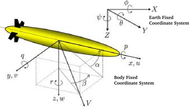
Figure 3-1 Linear and Rotational Axis System

To describe the state of a submarine requires knowledge of a significant number of variables. Firstly, its body fixed velocity vector = — both linear and angular components — (see Figure 3-1). These values are to be taken about a known, body-fixed origin. For the SUBOFF model referenced throughout this document, the origin is located as per the original DTRC model; on the axial

centreline, at the centre of rotation (Roddy, 1990). Secondly, its earth fixed position = , which allows the derivation of a vector ( ) for the (inherently earth fixed) gravitational components of weight and buoyancy. Thirdly, the control vector of forces and moments acting upon it (propulsion, dive & rudder planes) = . Fourthly, the physical characteristics of the vessel in terms of its

Earth Fixed Coordinate System

(31)

Page 19

inertial matrix , including the effect of any acceleration upon the surrounding fluid. From this inertial matrix, a matrix of the resulting coriolis and centripetal forces can be calculated directly. Finally, the damping response of the fluid must be accounted for, which is done via a damping matrix . In the vector form utilised by Fossen (1994), the resultant equations of motion can be written:

= − ( ) − ( ) − ( ) (3.1)

In this thesis, motion and forces are limited to the vertical plane. Given the form above and this limitation, much of the system of equations can be simplified. The body fixed velocity vector becomes = , the earth fixed position vector =

. The gravity vector, reduced to three dimensions and transformed into the body-fixed frame of reference (by a rotation ) becomes:

( ) =

( − )

−( − )

( − ) + ( − )

(3.2)

The inertial matrix , including both the rigid body and non-negligible added mass terms:

=

− 0

0 − −

− −

(3.3)

Note: values for the added mass terms , , , , can be determined by or derived through linear or cyclic acceleration tests.

The corresponding Coriolis matrix , derived directly from the mass matrix as per the methodology in Fossen (1994):

=

0 0 + +

0 0 − − −

− − + + − 0

(3.4)

The control vector = typically contains expressions of the forces actively exerted on the vessel, primarily those derived from propulsion and the action of the various dive planes and rudders. For example, the expression in Feldman’s (1979) general equations of motion reduces under these conditions to:

=

+ + + + +

+ + −

(3.5)

(32)

Page 20

of , , , , are given in Feldman, 1979). These terms assume a specific control surface arrangement and would have to be altered to capture an alternate form: see Healey & Lienhard (1993) for an alternate expression featuring rudders fore and aft, as well as utilising propeller rate rather than command speed.

The hydrodynamic damping matrix consists of nine terms which approximately express the non-linear nature of the damping forces imposed upon a submarine in the course of its motion. In this approximation process — seeking a sufficiently accurate yet simple representation of the forces modelled — a degree of art is expressed, leading to a number of alternate models being found in the literature and in practical use.

Assuming briefly a linear response, the results for the damping matrix are obtained by setting the velocity vector to = 0 0 , and then perturbing the components of that vector by some small amount independently. Under these conditions, the

following damping matrix is obtained:

( ) = (3.6)

This simple model works well in the condition where the velocity vector is

approximately 0 0 . However, in practice, it is desirable to be able model the response over a larger range than is covered sufficiently accurately by the

simplification made in assuming a linear response. In order to achieve this, rather than assess a single perturbation in each direction, each component is assessed across a range of values and a function fitted to those results. These response curves will be expressed as per Sen (2000) e.g. ⋆ is the variation in the axial force with

variation in axial velocity. Using this notation, ( ) is more fully expressed as:

( ) =

⋆ ⋆ ⋆

(3.7)

As mentioned in Chapter 2, Roddy (1990) summarises the experimental outcomes of a number of tests conducted on the SUBOFF model. In Figure 11 (reproduced below as Figure 3-2), the response obtained in the non dimensionalised axial force

(33)

[image:33.595.125.427.61.271.2]

Page 21

Figure 3-2 X' as a function of , Fig. 11 Roddy (1990)

This presents an approximately parabolic response for as a function of , (noting = sin , which is close enough to linear in this range not to substantively change the curve). Thus, for instance in Feldman’s (1979) equations for axial force, an expression is found approximating the response curve ⋆ (axial force across a range of normal velocity ), as , capturing this basic form with a single coefficient.

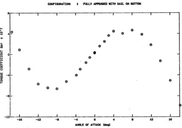
Not all response curves can be captured well using a single coefficient. Figure 3-3 below, reproducing Figure 13 from Roddy (1990), shows the response of ′ to changes in .

Figure 3-3 M' as a function of , Fig. 13 Roddy(1990)

[image:33.595.124.429.471.685.2]

(34)

Page 22

plane only. Doing this allowed the capture of the variation in pitch moment with direction of rotation that occurs due to the asymmetry of the body (primarily due to the presence of the sail). The selection of this more complex expression is an

example of mapping what in some cases are complex and noisy experimental results into a relatively simple yet sufficiently representative mathematical form. Feldman’s terms for the hydrodynamic response are:

( ) = ⋆

⋆ + | | | |+ +

⋆ + | | | |+ + | || | +

(3.8)

An alternate approach to evaluating these terms is as utilised in Jensen et al (1993) whereby a lookup table is created for each response curve. The lookup table has the advantage of more closely approximating the measured response, but at the cost of additional computation. Lookup tables can also be utilised in more than a single dimension to reduce approximation error where significant cross coupling between terms exists.

3.2 Sensitivity of Coefficients in typical manoeuvres

In order to judge whether the effects of a change in response due to the action of the free surface is:

a) sufficient to warrant the addition of a new term or modification of an existing term; and

b) sufficiently accurate in its modelling thereof; some quantifiable measure must be determined.

Sen (2000) reports on the sensitivity of a general submarine model to the various coefficients utilised therein. His paper sets out a methodology for the assessment of sensitivity in terms of the relative change in the modelled submarine path resulting from variation in each coefficient from its reference value. The sensitivities noted are derived from vessel response during overshoot and turning circle manoeuvres — typical trial manoeuvres. While alternative manoeuvres, reference coefficients, and systems of equations would inherently derive different results, the results obtained provide a basis for assessment of which coefficients are the most sensitive and thus the highest priority to assess for variation. The system of equations modelled in Sen are based loosely on Feldman’s equations and are thus largely similar to those utilised within this thesis.

(35)

Page 23

Chapters 4 and 6 in order to judge under what conditions it is necessary that each coefficient should be treated as variable in the near surface regime.

Table 3-1 Sensitivities of various coefficients (Table 4, Sen 2000)

4.914 3.154 2.305

2.025 1.597 1.290

⋆ 1.203 | | 1.046 0.988

0.979 0.959 0.959

0.953 | | 0.944 | | 0.933

⋆ 0.889 0.885 0.319

0.300

Note: Details on the derivation of these values can be found in Sen (2000). The vertical plane coefficients can be grouped roughly into four categories:

a) Pitch coefficients ( , );

b) Normal-force coefficients ( , , , , ⋆);

c) Shaping coefficients ( | | , , , , , | |, | | , ⋆, ); d) Axial-force coefficients ( , , )

Notably, no figure for the sensitivity of the equations to ⋆ ( in Sen, 2000) is provided. However, Perrault, Bose, O’Young & Williams (2003) suggests a maximum sensitivity of 0.387 in a similar series of tests, which will be utilised in this thesis. For comparison, they report a maximum sensitivity to ( , in Perrault et al, 2003) of 1.106, which is somewhat smaller than that reported in Sen (2000).

Some clear observations can be drawn. Variance of path due to coefficients of pitch is more significant than with heave, and linear coefficients (and control coefficients) are more sensitive than higher order terms. Still, other than the coefficients in (which as noted, were not stressed in these tests as much as say a crash stop under jammed controls) the sensitivity of all coefficients tested were within a factor of 4 of each other.

3.3 Consideration of the Effects of Proximity to the Free Surface

Let us assume that near the free surface the existing damping matrix calculation for submarine motion is modified by the consideration of position as well as velocity:

= − ( ) − ( ) − ( , ) (3.9)

Where ( , ) is a function of both position and velocity that represents the hydrodynamic effects inclusive of the interactive effects of the free surface upon the submarine.

(36)

Page 24

surface. There are two primary thrusts of the literature that will be referenced here: experimental results and theoretical development.

As noted in Chapter 2, the early experimental results of Weinblum et al (1936) reflected what had already been predicted by the theoretical considerations of Lamb and Havelock on the resistance of a submerged ellipsoid approximately 10 years earlier. Figures 3-4 and 3-5 (Weinblum et al, 1936) show residual resistance plotted against Froude Number for two different hull forms, at different submergences.

Figure 3-4 Resistance as a function of Froude Length Number, Model 1257, Weinblumet al(1936)

Figure 3-5 Resistance as a function of Froude Length Number, Model 1242, Weinblumetal(1936)

(37)

Page 25

[image:37.595.138.419.168.399.2] [image:37.595.130.426.447.658.2]

Similarly, from the results of work conducted by Crook (1994) — see Figure 3-6, showing lift coefficients plotted against Froude Number — and Neulist (2011) — see Figure 3-7, showing pitch moment plotted against Froude Number and submergence — it is evident that the functions for heave and pitch are likewise neither simple nor simply periodic in nature.

Figure 3-6 Lift Coefficient as a function of Froude Number and Submergence (Crook,1994)

Figure 3-7 Pitch Coefficient as a function of Froude Number and Submergence (Neulist, 2011)

Inspection of the results in these papers led to some simple observations relevant to the problem at hand.

(38)

Page 26

• The surface effect fades quite quickly with submergence and is negligible at depth;

• Change in submergence result in slight changes in the speed at which peaks and troughs occur.

The near surface effect on the submarine is composed of two components: change in pressure, and change in skin friction. In all cases tested as a part of this thesis, change in skin friction is less than 4% of the total variation, in most cases less than 1%. In assessing suitable mathematical functions for the change in pressure it is worth considering the results of potential theory.

Havelock (1928) formulated the function of the free surface under potential flow conditions over a doublet of strength submerged at a depth in a uniform flow of velocity .

( , )

= ₍ 2

+ ) /

+2 +

+

+4 ( − )

(3.10)

Where = / and is a dummy variable for integration.

Lazauskas (2005) utilised a simplified version of the above derived by Tuck (1971) where:

( , ) = ℜ / ( ) ( ) ( , , )

/ (3.11)

with ( ) = sec , ( , , ) = + sin and ( ) as the complex amplitude function derived by any of the various means noted in their paper. The function was found to develop rapid oscillations as | | → ₂, leading regular

(39)

Page 27

The first term in equation 3.10 above is simple and consideration will be given to treating this component of the waveform independently. Furthermore, equation 3.11 suggests that any effect due to the free surface will reduce exponentially with

submergence. This corresponds with wave theory for deep water, where the velocity field also reduces exponentially with depth.

3.3.1 Notation Selected for Free Surface Manoeuvring Coefficients

Given the general structure of the equations of motion near the free surface noted in Equation 3-9, ( , ) represents the matrix of the damping forces inclusive of the proximity, orientation and motion relative to the free surface. It is anticipated that the variation of pressure due to the generated waves during operations in the near surface will vary with submergence, velocity and attitude.

In describing the variation of an individual coefficient in the near surface region, Renilson (2015) utilises the notation ⋆( ⋆, ) , denoting the previously constant manoeuvring coefficient ⋆ as now a function of the pertinent components of when in the near surface region. This coefficient function can be computed either through the use of a multi-dimensional look up table, though some explicit function of , or some combination thereof.

Using this notation ( , ) can be written:

( , ) =

⋆_{( )} ⋆_{( )} ⋆_{( )}

(3.12)

3.4 Adoption of a General Form

Starting from the Feldman equations of motion (See Appendix C), the following equations have been adopted as standard equations of form for three degrees of freedom in the vertical plane. Each Feldman equation has been reduced to the three degrees of freedom within the vertical plane; i.e. = = = 0. In addition, the expressions for combined heave/pitch found in Gertler & Hagen (1967) are adopted rather than the integral forms utilised in the later Feldman model as these moved away from the coefficient-based nature of the model and have not been widely adopted. Control surface forces are neglected; i.e. = = = 0. All terms are herein expressed in their non-dimensional forms for consistency with current conventions.

Given constant self-propulsion speed, (i.e. = , = ) the propulsion function is reduced to:

(40)

Page 28

A

XIAL

F

ORCE

E

QUATION

( − ) + = (3.14)

⋆ + − − + +

+( ′ − ′)

N

ORMAL

F

ORCE

E

QUATION

( − ) − + = (3.15)

⋆ + + | | | |+ + | | | |

+ + _{| |} | | + ( − ) + ( − )

P

ITCH

M

OMENT

E

QUATION

− ( + ) − ( + ) = (3.16)

⋆ + | | | | + | | | | +

+ + | | | | – ( + )

+( − ) − ( − )

These equations will be used from here on as the general equations of vertical plane motion for a submarine in deep water.

3.5 Compiling a Complete Model of the Near Surface Static Response

The compilation of a first model of the near surface response of a submarine requires the derivation of response curves in three axes (axial, normal, pitch). From the sensitivity study by Sen (2000) it is known that any changes that affect the forces imposed by the control vector are significant. Changes to the added mass coefficients in the near surface must also be considered.

3.5.1 Matrix for Assessment of Coefficient Consequence

In order to be able to address the significance of any change in response due to the presence of the near surface, a metric of consequence is utilised. As noted in Section 3.2, the performance of the model is sensitive to each coefficient to distinctly

different degrees. Furthermore, as could be anticipated, the relative variance of each coefficient under the influence of the near surface is markedly different from

coefficient to coefficient. As such, for the assessment of each coefficient , a Consequence ( ) will be determined as the product of the sensitivity ( ) of the model to that coefficient and the scale of change in that consequence noted as a result of the studies conducted in Chapters 4 and 6.

Numerical calculation of manoeuvring coefficients for modelling the effect of submarine motion near the surface