PP 2002 13: Construction by Description in Discourse Representation

Construction by Description in Discourse

Representation

Noor van Leusen and Reinhard Muskens

Abstract

This paper uses classical logic for a simultaneous description of the syntax and semantics of a fragment of English and it is argued that such an approach to natural language allows procedural aspects of lin-guistic theory to get a purely declarative formulation. In particular, it will be shown how certain construction rules in Discourse Represen-tation Theory, such as the rule that indefinites create new discourse referents and definites pick up an existing referent, can be formulated declaratively if logic is used as a metalanguage for English. In this case the declarative aspects of a rule are highlighted when we focus on the model theory of the description language while a procedural perspec-tive is obtained when its proof theory is concentrated on. Themes of interest are Discourse Representation Theory, resolution of anaphora, resolution of presuppositions, and underspecification.

1

Introduction

1991) and related formalisms (including (Muskens, 1996)) it is necessary to assume that syntactic input to the semantic component comes pre-indexed, with co-indexation between antecedents and dependent elements represent-ing anaphoric linkrepresent-ing.

The question of declarativity versus procedurality is related to the ques-tion which roles the main branches of logic can play in linguistic theory. There is a natural tendency to associate linguistic semantics with model theory and linguistic syntax with proof theory. Montague’s work is a prime example of the first association, while the connection between natural lan-guage syntax and proof theory is apparent from the widespread use of con-text free grammars in syntactic theory, from the derivations in early trans-formational approaches, and, even more explicitly, from Lambek’s categor-ical calculi (Lambek, 1958; Moortgat, 1997). However, it is also fruitful to make cross-combinations. This becomes apparent, for example, when we turn to the ‘model-theoretic syntax’ of (Blackburn, 1993; Blackburn, Gar-dent and Meyer-Viol, 1993; Rogers, 1996; Blackburn and Meyer-Viol, 1996) and others. Model-theoretic syntax studies the model theory of syntactic structures such as trees and feature structures. In a similar spirit (Kur-tonina, 1995) defines various forms of Kripke semantics for the language of Lambek categorial grammar, and works out the model theory and corres-pondence theory of such systems, thus also giving a model-theoretic twist to an enterprise whose main focus is on natural language syntax. Conversely, proof-theoretic approaches to natural language semantics also abound. Some accounts are purely proof-theoretic, such as the approach of (Ranta, 1994), which is based on Martin-L¨of’s intuitionistic type theory. Other applications of proof theory to linguistic semantics seek to supplement existing model-theoretic accounts. As an example of the latter the type-shifting proposals (Partee and Rooth, 1983) and (Hendriks, 1988) can be mentioned. These proposals have a definitely proof-theoretic flavour and are related to the (undirected) Lambek Calculus.

introduces an orthogonality between, on the one hand, the proof theory and model theory of the describing logic, and, on the other, the syntax and semantics of the fragment described. Our aim is to develop a combined logic of form and meaning; when focussing on its proof theory we get its procedural aspects, if its model theory is focused on, its declarative aspects are highlighted. This, of course, is the normal duality of proof and structure in logic.

A Logical Description Grammar (LDG) will be a logical theory G, set up with the intention that whenever we have a logical sentence IT stating some simple properties of a textT, the combined theoryG+IT describes the syntax and semantics ofT. We will assume here that the models of G+IT

contain trees decorated with semantic values; a function (or, in fact, family of functions) σ will associate values with tree nodes. The logic talks about natural language semantics andnatural language syntax. In its models we get semantically annotated trees (this in addition to the usual objects and relations) and in its proof theory we can reason about these.

As was argued extensively in (Muskens, 2001), underspecification natu-rally falls out of this view. Since a descriptionG+IT can have more than

one model, the syntax and semantics of T may remain underspecified. In particular, it can be shown that, with the right set-up, certain stages in the reasoning process that takesG+IT as its point of departure are closely

anal-ogous to the Underspecified Discourse Representation Structures of (Reyle, 1993). There is no need to postulate a separate structural level of the latter, we get UDRSs for free if the hearer’s simultaneous reasoning about the syn-tax and semantics of an input expression is modeled. We conclude that the description view on Discourse Representation explains why UDRSs emerge. No stipulation of such structures is necessary.

The organization of this paper is as follows. In the next section we start with defining and explaining the ‘Logical Description Grammars’ of (Muskens, 2001); it will be discussed how input descriptionsIT are obtained

Variable Type x, y, z e

k ν

v π

Variable Type

i, j s

c st×πt

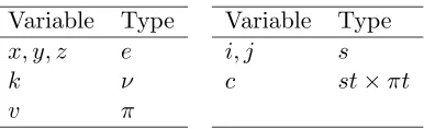
Table 1: Variables used in this paper will have types as indicated.

and how underspecified DRSs can be identified with certain descriptions. The paper ends with a conclusion and an appendix gives a small grammar fragment.

2

LDG: Input Descriptions and Axioms

In this section and in section 4 we will give an overview of the Logical De-scription Grammars (LDGs) developed in (Muskens, 1995; Muskens, 1999; Muskens, 2001).1 _{We describe a system that is closely related to the one}

given in the last of these papers, but make some choices of design that slightly deviate from those that were made there. For more details and motivation the reader is nevertheless referred to (Muskens, 2001).

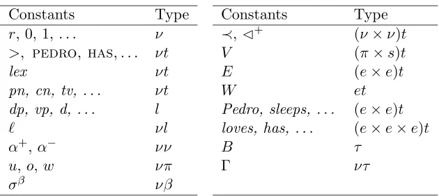
We work in classical type logic with ground types e (entities), ν (tree nodes), l (tree labels), π (registers), and s (states). Since we will have oc-casion to use many variables and constants in these types and in complex types composed out of these primitive ones, it will be convenient to have typographical conventions of the form: ‘whenevervis used, it will be a vari-able of typeπ.’ Table 1 gives an overview of such typographical conventions used for variables and Table 2 gives a similar overview for constants.

It will be expedient to have pairing and projectionin the logic. We will assume that wheneverAis a term of typeα andB a term of typeβ,hA, Bi

is a term of typeα×β. Also, whenever A is a term of type α×β, fst(A) will be a term of typeα (denoting the first element of the denotation of A) and snd(A) a term of type β (denoting the second element). These terms will have the obvious semantics.

1_{As far as we are aware (Muskens, 1995), presented at the Prague session of the}

Constants Type r, 0, 1, . . . ν >, pedro, has,. . . νt

lex νt

pn, cn, tv, . . . νt

dp, vp, d, . . . l

` νl

α+_,α− _νν

u,o,w νπ

σβ _νβ

Constants Type

≺,¢+ _(ν×ν)t

V (π×s)t

E (e×e)t

W et

Pedro, sleeps, . . . (e×e)t

loves, has, . . . (e×e×e)t

B τ

Γ ντ

Table 2: Some constants used in this paper and their associated types. Here β varies over types andτ is an abbreviation of πt×(st×πt)t (the type of DRSs).

2.1 Input Descriptions

Descriptions in our approach will consist of two parts. The first part will be a grammar G consisting of certain axioms and a lexicon. This part is not supposed to vary and models a hearer’s grammatical knowledge. The second part will be the description IT of an observed text T. This input

description can be obtained in the following way. Suppose that the text that is to be described starts with (1).

(1) Pedro has a mule

Discourse participants reason about the trees that are possibly connected with a given discourse. The input description only concerns the lexical elements of such trees. We shall assume that lexical elements can be words or discourse relations,2 _{including a special unary discourse relation signifying}

that the discourse has started. Upon hearing (1) a discourse participant can draw certain conclusions. First, she may conclude that the discourse has

2_{We are simplifying matters considerably here. In a fully fledged discourse model,}

we would distinguish between discourse connectives, such as ‘and’, ‘but’, ‘because’ and ‘either . . . or’, and the discourse relations which they denote or partly specify, such as

indeed started and that the start element, which she may give a name, say 0, must therefore be present. She draws the conclusion in (2a). Here ‘>’ stands for the predicate ‘is the start element’ and ≺denotes precedence in trees. Secondly, there is a lexical element ‘Pedro’, which came just after the start. So the tree must have a lexical node labeled ‘Pedro’. Our hearer gives it an arbitrary node name, say 1, and concludes (2b), in which≺1 is

immediate precedence (i.e.n≺1n0abbreviatesn≺n0∧¬∃k[n≺k∧k≺n0]).

(2) a. >(0)∧ ¬∃k k≺0

b. pedro(1)∧0≺1 1

c. has(2)∧1≺1 2

d. a(3)∧2≺13

e. mule(4)∧3≺1 4

In a similar fashion the hearer adds (2c)–(2e) to her stock of beliefs, after which she may perhaps hypothesize that the end of the discourse has been reached already, hypothetically adding (3). (Addition of such an ‘end’ state-ment will make interpretation of the text heard sofar possible, as we will see below.)

(3) ¬∃k4≺k

Of course, the discourse may in fact continue, say with (4).

(4) He feeds it

Assuming that our hearer recognizes that this is a new sentence and not a continuation of previous material, she will now stipulate the existence of a discourse relation. In this paper the only binary discourse relation that will be introduced is simplesequencing, but see (Duchier and Gardent, 2001; Webber et al., 2001; van Leusen, 2003) for more extended treatments of discourse relations in grammar systems closely related to the present one. The set of descriptions is now continued as follows.

(5) a. seq(5)∧4≺15

b. he(6)∧5≺16

d. it(8)∧7≺1 8

The hypothesis in (3) can no longer be upheld, of course. But at this point it can be replaced by the hypothesis in (6).

(6) ¬∃k8≺k

The input description associated with a given text T will consist of the conjunction of all descriptions collected in this way, including the hypothesis that no material follows T. For example, the input description for ‘Pedro has a mule. He feeds it.’ will be the conjunction of the logical sentences in (2), (5), and (6).

2.2 Axioms

The knowledge modelled by a grammar G can be separated into lexical knowledge (to be discussed in section 4) and general grammatical knowledge. We will assume here that the latter contains at least the following.

• Knowledge about linguistic trees;

• Knowledge about the ‘anchoring’ of tree nodes; anchoring provides a mechanism that makes lexical items combine;

• Knowledge about semantics.

For each of these forms of knowledge we provide axioms.

Axioms for Trees AxiomsA1–A5 below (see also (Cornell, 1994; Backofen, Rogers and Vijay-Shankar, 1995)) make the binary relations ¢+ and ≺

behave like proper dominance and precedence in linguistic trees, with r as root (k1¢∗k2 will be an abbreviation ofk1¢+k2∨k1 =k2). Nodes in such

trees may belabeled with a labeling function`. For example, we may want to say that nodenis labeleddpby stating`(n) =dp. Axiom 6 rules out that label names such asdpand vp corefer. Instantiations of this axiom scheme will be sentences like dp6=vp and ap6=pp, etc. Axiom A7, lastly, requires lexical nodes to be leaf nodes. i.e. nodes that do not properly dominate any other node.

A1 ∀k r¢∗_k

A3 ∀k1k2[k1 ≺k2∨k2 ≺k1∨k1¢+k2∨k2¢+k1∨k1 =k2]

A4 ∀k1k2k3[[k1¢+k2∧k1 ≺k3]→k2 ≺k3]

A5 ∀k1k2k3[[k1¢+k2∧k3 ≺k1]→k3 ≺k2]

A6 c16=c2, ifc1 andc2 are distinct label names

A7 ∀k1k2[lex(k1)→ ¬k1¢+k2]

The Anchoring Axiom The next axiom plays an essential role in the mecha-nism that combines lexical elements into larger units. The idea is that every tree node must be licensed ‘from below’ by a lexical element. Each node should also be licensed ‘from above’ by a lexical element. A node that is licensed ‘from below’ can be thought of as ‘produced’ by the lexical element, while nodes licensed ‘from above’ need to be ‘consumed’. Typical examples of the latter are argument nodes. The idea essentially stems from Catego-rial Grammar, where arguments have a negative occurrence in an element’s category and must match with positive occurrences of other categories. (For the producer / consumer metaphor, see Linear Logic (Girard, 1987), which is closely related to Categorial Grammar.)

If a node k0 _{licenses a node k ‘from below’ we write α}+_{(k) = k}0_{; that}

k0 _{licences k ‘from above’ is expressed by α}−_{(k) = k}0_{. α}+_{(k) is called the}

positive anchor of k; α−_{(k) its negative anchor. The axiom states that all}

positive and negative anchors must be lexical.

A8 ∀k[lex(α+(k))∧lex(α−(k))]

The effect of this axiom will become apparent in section 4.

Semantic Axioms Three kinds of axioms will be needed for our semantics. There will be axioms for the mechanism of binding, axioms forworlds, and an axiom that plays a role in assigning local contexts to tree nodes. The notion of a local context derives from (Karttunen, 1974). Here it will be a Discourse Representation Structure. The local context of a node should well be distinguished from the semantics of that node.

A9, A10 and A11 implement a version of the axioms for binding in (Muskens, 1991; Muskens, 1996; Muskens, 2001). We writeV(v, i) for ‘the value of registerv in state i’ and if δ1, . . . , δn are terms of type π, we write

differ at most inδ1, . . . , δn’).3 The first axiom says that, in each state, each

register can be updated selectively, i.e. its value can be set to anyxwhile the values of other registers can remain unchanged. This axiom makes states and registers essentially behave as assignments and variables in predicate logic. (The last remark is fleshed out in (Muskens, 2001).)

A9 ∀i∀v∀x∃j[i[v]j∧V(v, j) =x]

A10 ∀kk0_ρ(k)6=ρ0_(k0_{), ifρ, ρ}0 _{∈ {u, o, w} are distinct}

A11 ∀k1k2[ρ(k1) =ρ(k2)→k1=k2], ifρ∈ {u, o, w}

We letu,o, andwbe functions from nodes to registers. AxiomA10 ensures that the images of these functions are disjoint, while A11 requires each to be injective. In this way we make sure that fresh registers come with each node. This in turn will make it easy to let indefinites be associated with new discourse referents. The values of u will typically be associated with new referents, while the values of o are referents that belong to the ‘background’ of the discourse. The values ofw are registers that can store

worlds. In this paper we will only use w(r), the w value of the root.4 A notational convention that we find useful is to write arguments ofu,o, and was subscripts, e.g. u3 instead ofu(3), wr instead ofw(r) etc.

While states correspond to assignments and registers correspond to vari-ables, the notion of a possible world of course corresponds to the technical notion of amodel. We will make some use of possible worlds here, but will not change the logic—a step often associated with their introduction. In-stead we will consider possible worlds to be objects of type e, i.e. we will simply take them to be (abstract) entities. The predicate letterW will be used for the predicate ‘is a world’ and E will be an existence predicate, so that E(x, y) stands for ‘object x exists in world y’ and λx E(x, y) is y’s domain. In our semantics we shall make use of a (finite) setL of predicate letters ({Pedro, has, mule, feeds, . . .}) all of whose arguments are of typee and whose last arguments are to be interpreted as worlds. E.g.has(x, y, z) should be read as ‘xhasy in worldz’. The following axiom scheme requires that last arguments indeed are worlds and, somewhat rigorously, demands

3_{v must be chosen as the first variable in some fixed ordering which is not free in}

δ1, . . . , δn.

4_{But in extensions containing modal operators it would be natural to use other values}

that all other arguments of an L relation denote objects in this world’s domain.5

A12 ∀x1. . . xny[R(x1, . . . , xn, y)→(W(y)∧E(x1, y)∧. . .∧E(xn, y))],

for each R∈ L

WhileA9 in a sense required there to be enough states present for the bind-ing mechanism to work, the next axiom scheme puts similar requirements on the sets of individuals and worlds. Since we want to use our logic as a metalanguage for English, it would be nice to have a notion of entailment around at the level of the logic (of course we already have a notion of entail-ment at the ‘metametalevel’—the present level of description). Entailentail-ment is obtained by quantification over models, or, since the latter’s role is played by worlds at the logic’s level, by quantification over worlds: an entailment holds if the conclusion is true in all worlds in which the premises are true. But this requires all worlds to be available; otherwise counterexamples to an entailment might be missed. A requirement that really ensures all or all countable worlds to be present in all models does not seem to be formulable with finitary and first order means and since we do not wish to use too heavy artillery we therefore make do with a requirement that at least all

finite worlds be present; for our natural language application this seems a very reasonable approximation.6

This will be ensured in the following way. Define an L-atom to be an atomic formula R(t1, . . . , tn) with R∈ L. An L-literalis an L-atom or the

negation of an L-atom. The following axiom scheme may be instantiated by any number of variables x1, . . . , xn and any conjunction of L-literals

ϕ(x1, . . . , xn, y) satisfying the conditions stated.

A13 ∃x1. . . xny[W(y)∧x1 6=x2∧x1 6=x3∧. . .∧xn−16=xn∧ ∀x[E(x, y)↔(x=x1∨. . .∨x=xn)]∧ϕ(x1, . . . , xn, y)],

whereϕ(x1, . . . , xn, y) is a conjunction of L-literals with at most x1,

. . . , xn and y free that does not contain both an L-atom and its

negation.

5_{This will serve present purposes. That the requirement needs to be fine-tuned can be}

seen from such classic examples such as ‘worship’, where the object argument need not exist. The axiom also will need to be adapted if accessibility relations between worlds are considered, something we shall not do in this paper.

6_{Compare (van Benthem, 1986), where it is argued that, in order to keep complexity}

This axiom scheme will have instantiations such as, say,

∃x1x2x3y[W(y)∧x1 6=x2∧x1 6=x3∧x2 6=x3

∧ ∀x[E(x, y)↔(x=x1∨x=x2∨x=x3)]

∧has(x1, x2, y)∧ ¬has(x2, x3, y)∧mule(x2, y)∧hay(x3, y)] .

Thus every finite world is stipulated to exist, as we can easily produce an exhaustive description in this way (a so-called ‘diagram’). Note that this does not only ensure the existence of many worlds but also the existence of a multiplicity of states. Since, according toA9, each register of a state can be selectively updated with type evalues, and since worlds are typeeobjects, each state will have many variants differing only from it in the value of the registerwr.7

We turn to the axiom about local contexts. The local context of a node kwill be a Discourse Representation Structure Γ(k) that can be computed from the local contexts and semantics of other nodes. A14 states that the local context of any non-S or non-T node (T is the category of texts) equals the local context of its mother (if it has one). Here k1 ¢k2 abbreviates

k1¢+k2∧ ¬∃k[k1¢+k∧k¢+k2], i.e. ¢denotes the immediate dominance

relation.

A14 ∀k1k2[[k1¢k2∧`(k2)6=s∧`(k2)6=t]→Γ(k2) = Γ(k1)]

How the local contexts of S nodes and T nodes are to be computed will be regulated in the lexicon.

3

A Fine-grained Compositional DRT

In this section we will give some definitions that will make key concepts of Discourse Representation Theory available. The definitions are based upon the semantic axioms that were given above and the DRT concepts that result will be needed in our further discussion of Logical Description Grammars and it is for this reason that we interrupt the treatment of the latter.

The approach here will have much in common with that of (Muskens, 1996), but will also differ from it in an important respect. What the two approaches have in common is that both are based on a transcription of truth conditions for DRT, carried out within an axiomatic extension of type logic (minor variations of the binding axioms that are relevant here are also

7_{States that have worlds inu ororegisters are not formally excluded, but are of no}

present in (Muskens, 1996)). The difference between the two treatments re-sults from the fact that while in (Muskens, 1996) the DRT truth conditions that were transcribed were those of (Groenendijk and Stokhof, 1991, defini-tion 26), here we will use a variant of the semantics in (Zeevat, 1989). The reason for this difference in treatment lies not only in our wish to emphasize the flexibility of the ‘transcription’ approach, but also in the fact that in this way we get a more fine-grained DRT semantics (in the sense that we get stronger requirements on the identity of DRSs), which suits our present purposes better.

Some abbreviations introducing set-theoretic notation will come in handy.

Definition 1 LetA1, . . . , Anbe terms of some typeαand letXbe the first

variable of that type not free in these terms, then

{A1, . . . , An} abbreviates λX[X=A1∨. . .∨X =An].

Furthermore, letA and B be terms of some type (α1(· · ·(αnt)· · ·)) and let

X1, . . . , Xn be variables such that eachXi is of tyeαi. Then

A∪B abbreviates λX1. . . Xn[AX1. . . Xn∨BX1. . . Xn],

A∩B abbreviates λX1. . . Xn[AX1. . . Xn∧BX1. . . Xn],

A⊆B abbreviates ∀X1. . . Xn[AX1. . . Xn→BX1. . . Xn].

In (Zeevat, 1989) the semantic value of a Discourse Representation Structure K is a pair consisting of (a) a set of discourse referents (the universe of K) and (b) a set of assignments. The latter consists of all those assignments that verify all conditions in K. This could easily be transposed to the present set-up by letting the first part of any DRS K consist of a set of registers (typeπt) and its second part of a set of states (typest), so that the type of DRSs would beπt×st. However, we opt for a variant of this approach and will deviate from Zeevat’s treatment in two respects. Firstly, we will follow (Visser, 1994) in keeping track of the free discourse referents in any DRS or condition (see also (Van Eijck and Kamp, 1997)). This can be done by letting conditions be pairs of (a) sets of states and (b) sets of registers (those that are free in the condition). The type of a condition will then become st×πt.

is argued, for example, that the effect of a correction can be a selective downdate of a DRS, with some conditions disappearing while others remain. With these modifications the type of DRSs becomesπt×(st×πt)t, which we will often abbreviate asτ. The alternative formalization will give stronger identity criteria on DRSs.

Given that the free referents of a condition form its second element, the free referents of any DRSKcan easily be computed: these are the ones that are free in some condition of K but are not in the universe of K. A DRS will be proper if it has no free referents. These notions are made available to the logic with the following definitions.

free(K) abbreviates λv∃c[¬fst(K)(v)∧snd(K)(c)∧snd(c)(v)]

proper(K) abbreviates ¬∃vfree(K)(v)

The two following notions play a key role in the algebra of Discourse Rep-resentation Structures.

Definition 2 LetK and K0 _{be terms of typeτ.}

K⊕K0 abbreviates hfst(K)∪fst(K0),snd(K)∪snd(K0)i

KvK0 abbreviates fst(K)⊆fst(K0)∧snd(K)⊆snd(K0)

We will typically be interested in typeτ objects h{δ1, . . . , δn},{γ1, . . . , γm}i

with a finite universe{δ1, . . . , δn}and a finite set of conditions{γ1, . . . , γm}.

Such DRSs we prefer to write as [δ1. . . δn|γ1, . . . , γm], in a way reminiscent

of the usual ‘box’ notation for DRSs.

While we essentially follow the Zeevat approach to the semantics of Dis-course Representation here, the dynamic treatment of (Groenendijk and Stokhof, 1991; Muskens, 1996) is still available. The Groenendijk-Stokhof interpretation of a DRS K can be defined as the relation gs(K) between statesiand j such that idiffers fromj at most as far as the universe of K is concerned and j verifies all conditions in K. In other words, gs(K) can be taken to abbreviate

λij(∀v[¬fst(K)(v)→V(v, i) =V(v, j)]∧ ∀c(snd(K)(c)→fst(c)(j))).

On the finite DRSs we are interested in, this leads to the more readable equation

gs([δ1. . . δn|γ1, . . . , γm]) =λij(i[δ1. . . δn]j∧fst(γ1)(j)∧. . .∧fst(γm)(j)).

Boolean⊕rules; the latter is a relational algebra with relational composition as one of its natural operations.

A DRS K istrue in a state iif there is a j, differing from i at most as far as the universe of K is concerned, such that j verifies all conditions in K. We will writetrue(K) for λi∃j gs(K)(i)(j). true(K) therefore denotes the domain of gs(K) and

true([δ1. . . δn|γ1, . . . , γm]) =λi∃j(i[δ1. . . δn]j∧fst(γ1)(j)∧. . .∧fst(γm)(j)).

The notion of DRS truth immediately leads to a notion of DRS consequence: K0 _{is said to follow from K if A1, . . . ,A14|=true(K)⊆true(K}0_{), i.e. if K}0

is true in all statesiin which K is true, in any model of the axioms.8 _This

notion can be relativised to any description D by saying that K0 _follows

from K given D if D,A1, . . . ,A14 |= true(K) ⊆ true(K0_{). It will be seen}

shortly how a similar notion can be obtained on the level of the describing logic.

Until now we have not paid much attention to the internal structure of DRSs, but the next definition gives notation for conditions.

Definition 3 Let R ∈ L, let δ1, . . . , δn be terms of type π (discourse

referents), and letK and K0 _{be terms of typeτ (DRSs). Then}

R{δ1, . . . , δn} abbreviates hλi.R(V(δ1, i), . . . , V(δn, i)),{δ1, . . . , δn}i

δ1 is δ2 abbreviates hλi.V(δ1, i) =V(δ2, i),{δ1, δ2}i not K abbreviates hλi.¬true(K)(i),free(K)i

K ⇒K0 abbreviates not (K⊕[|not K0])

K or K0 abbreviates htrue(K)∪true(K0),free(K)∪free(K0)i

Note that R{δ1, . . . , δn} predicates R of the values of δ1, . . . , δn in some

state, not of these registers themselves. We shall writeR{δ, wr} aswr:Rδ

andR{δ1, δ2, wr} aswr:δ1Rδ2.

Let us consider the sublanguage of typest×πtand typeτ terms that is given by the following Backus-Naur form, and dub it theDRT sublanguage. Here theδ range overπ terms that have the formρ(n), whereρ∈ {u, o, w}

andn is a node name. TheR are taken fromL.

γ ::= R{δ1, . . . , δn} |δ1 is δ2 |not K|K ⇒K0 |K or K0

K ::= [δ1. . . δn|γ1, . . . , γm]

8_{This gives an existential interpretation to all discourse referents that are present in}

It is useful to know that there are simple truth-preserving translations from the DRT sublanguage to predicate logic. The following one is taken from (Muskens, 1996) (but see also (Kamp and Reyle, 1993)).

Definition 4 Let†be a function that injectively maps eachδ to a variable of typee. The function tr from st×πt terms in the DRT sublanguage to predicate logical formulas and the functionwp, which takes a pair consisting of a τ term and a predicate logical formula and yields a predicate logical formula, are defined as follows.

tr(R{δ1, . . . , δn}) = R(δ†1, . . . , δn†)

tr(δ1 is δ2) = δ†1=δ † 2 tr(not K) = ¬wp(K,>)

tr(K⇒K0) = ¬wp(K,¬wp(K0,>))

tr(K or K0) = wp(K,>)∨wp(K0,>)

wp([δ1. . . δn|γ1, . . . , γm], χ) = ∃δ†1. . . δ†n[tr(γ1)∧. . .∧tr(γm)∧χ]

For any formulaϕ and state variable i, let ϕi _{be the result of substituting}

V(δ, i) for δ†_{, for each δ}† _{that is free inϕ. The following holds.}

Theorem 1 Let K be a τ term in the DRT sublanguage and let i be an arbitrary type svariable. Let Γcontain all statements δ 6=δ0_{, for every pair}

δ,δ0 _{of syntactically different discourse referents in K. Then}

Γ,A1, . . . ,A14|=wp(K,>)i↔true(K)(i)

The disequality statements are needed: If, say, 12 and 9 corefer, it fol-lows that [u12 | wr:muleu9] = [u9 | wr:muleu9], but the translation

would not preserve this. In practice this will be no limitation at all. For a proof of the theorem, use induction on complexity in the DRT sub-language construction to show that, given the axioms and disequalities,

wp(K, χ)i _{↔ ∃j[gs(K)(i)(j) ∧χ}j_{] and tr(γ)}i _{↔ γ(i), for all K and γ.}

This can be shown using the methods of (Muskens, 1996; Muskens, 2001). In the next section we will set up a logical mechanism that will assign DRSs or λ-terms involving DRSs to nodes as their semantic values. At many levels the special discourse referent wr for worlds will be free in such

DRSs. However, it will be ensured thatwr is always present in the universes

is to require that a context contains certain material. For example, for lexical nodes k that carry the proper name ‘Pedro’, we will demand that [ok |wr:Pedrook]vB. Another possibility is that a context is required to

bear a certain logical relation to another DRS K, where K typically does not have wr in its universe. Below we will have a brief look at Karttunen’s

theory of presuppositions, which provides an example, as it requires that presuppositionsfollow from their local context.9

These considerations make it necessary that logical relations such as entailment and consistency can be expressed or approximated at the level of the describing logic, but this has essentially been taken care of in the previous section. Suppose that K is a DRS with wr in its universe, while

K0 does not have wr in its universe. Then the condition K ⇒ K0

quan-tifies over possible worlds. This is best illustrated with an example: let us take K to be [wro1 | wr:muleo1], ‘there is a mule’, and let K0 be

[u2 |wr:farmer u2, wr:u2 owns o1], ‘some farmer owns the mule’, so that

K0 _{should not be made to follow from K. Then, for arbitrary i,}10

tr(K⇒K0)i =∀y∀x1[mule(x1, y)→ ∃x2[farmer(x2, y)∧owns(x2, x1, y)]] .

In view ofA12 this is equivalent with

∀y[W(y)→ ∀x1[(mule(x1, y)∧E(x1, y))→

∃x2[E(x2, y)∧farmer(x2, y)∧owns(x2, x1, y)]]],

from which it is seen that indeed quantification over worlds is involved. Note that A13 immediately provides a singleton-domain counterexample to this purported strict implication and in general it will give finite counterexamples if there are such.

Conditions K ⇒ K0 _{are of type st×πt and we will typically want to}

state conditions on thet level. The following definition adds the necessary quantification over states / assignments.

Definition 5 LetK and K0 _{be terms of typeτ.}

K|³K0 abbreviates ∀ifst(K⇒K0)(i)

9_{A second example that springs to mind are the consistency and informativity}

(non-entailment) requirements in Van der Sandt’s theory of presupposition. An extension of our theory that would allow for local and intermediate accommodation would also make it possible to give a declarative version of Van der Sandt’s theory. A third example are the felicity constraints associated with discourse relations in (van Leusen, 2003), which are also formulated in terms of entailment and consistency. It turns out that while some discourse relations require consistency and informativity, others, such asdenial andconfirmation, impose opposite constraints.

4

LDG: Lexical Descriptions and Reasoning

We return to our exposition of the mechanics of LDG. The main themes will be the LDG lexiconand an explanation of the kind of reasoning that LDG allows.

4.1 Lexical Descriptions

There will be two kinds of lexical description, classifying descriptions and

elementary tree descriptions. Of these, the elementary tree descriptions carry most information, but the classifying descriptions play a useful role in connecting elementary tree descriptions with open class words.

Classifying Descriptions In (7) classifying descriptions for the open class words Pedro, has, and mule are given. (7a) states that whenever a nodek carries the word has, it must be classified as a transitive verb (tv) and its semantics σπ(πτ)_{(k) is λv}0_{λv[ |w}

r:v has v0]. (If α is a type, we will let σα

denote a function from tree nodes to objects of typeα.) The description for

mule in (7b) is similar, but the word is classified as a common noun (cn) and its semantics has a different type.

(7) a. ∀k[has(k)→(tv(k)∧σπ(πτ)_{(k) =λv}0_λv[|w

r:v has v0])]

b. ∀k[mule(k)→(cn(k)∧σπτ_{(k) =λv[|w}

r:mulev])]

c. ∀k[pedro(k)→(pn(k)∧σπ_{(k) =o}

k∧[ok|wr:Pedrook]vB)]

The classifying description for Pedro in (7c), lastly, is of a slightly differ-ent nature. Here the semantics is set to the discourse referdiffer-ent ok, but

an additional requirement enforces that the global context or background

of the discourse, for which we use the typeτ constant B, contains the DRS [ok|wr:Pedrook]. This in fact implements the usual DRT requirement that

discourse referents connected with names must be present in the universe of the main DRS and that any descriptive material connected with such discourse referents must likewise be available globally.

of (Vijay-Shankar, 1992; Rambow et al., 1995).11 An elementary tree de-scription states what must be true in any acceptable structure if some lexical node has certain given properties.

(8) ∀k[tv(k)→ ∃k1k2k3k4k5[`(k) =v∧`(k1) =s∧`(k2) =dp∧

`(k3) =vp∧`(k4) =vp∧`(k5) =dp∧∆(k1, k2, k3)∧∆(k4, k, k5)∧

k3¢∗k4∧σ(k4) =σ(k)(σ(k5))∧σ(k1) =σ(k3)(σ(k2))∧

k←+-{k, k1, k4} ∧k

−

←-{k, k2, k3, k5}]]

For example, (8), which uses the abbreviations in Definition 6 below, is an elementary tree description saying that whenever a tree contains a transitive verb, it must have certain other properties as well. The transitive verb must be labeled ‘V’, it must have a dominating node labeled ‘VP’, which in turn dominates a node labeled ‘DP’, etc. The description also contains anchoring information and semantic information.

Definition 6

∆(k, k0, k00) abbreviates k¢_k0_∧k¢_k00_∧k0 _≺k00

t←+-{t1, . . . , tn} abbreviates ∀k(α+(k) =t↔(k=t1∨. . .∨k=tn))

t←−-{t1, . . . , tn} abbreviates ∀k(α−(k) =t↔(k=t1∨. . .∨k=tn))

In general, an elementary tree description will have the form

∀k[cond(k)→ ∃k1. . . kn[χ(k1. . . kn)∧k

+

←-{k₁0, . . . , k_p0} ∧k←−-{k₁00, . . . , k_q00}]]

wherecondis some condition,χis a conjunction of formulas, and{k0

1, . . . , kp0}∪ {k00

1, . . . , kq00} ={k, k1, . . . , kn}. The condition cond can be a predicate like

tvorcn, associated with a whole class of elementary trees, it can be one of the discourse elements >or seq, but also any of the predicates associated with words (such aspedro,has, etc.).

A Simple Graphical Notation Even with the abbreviations of Definition 6 in place elementary tree descriptions such as the one in (8) are unwieldy. It is therefore expedient to change to a graphical notation that is easier to work with even if it is somewhat less precise. The picture in (9) is an alternative representation of the description in (8).

11_{For the relation between Tree Adjoining Grammars, D-Tree Grammars and the present}

(9) tv: _S+

k1

σk3(σk2)

DP− k2

VP− k3

VP+

k4

σk(σk5)

V3

k DP−k5

The conventions that were followed in obtaining (9) from (8) are the follow-ing.

1. Nodes are labeled as usual and node names (variables or constants) are given as subscripts.

2. Solid lines stand for immediate dominance (¢_{) relations. Left-right}

ordering between sisters or between terminal nodes stands for prece-dence (≺). Dashed lines stand for dominance (¢∗_).

3. Nodes which are positively but not negatively anchored to the lexi-cal node in an elementary tree description are marked +, while nodes which are negatively but not positively anchored are marked−. Nodes which are anchored both ways are saturated and unmarked. The situ-ation that a node is not anchored at all will never occur and the anchor itself may be marked with a3_{. It is understood thatk←}+_{-{k1, . . . , kn}}

is asserted ifkis the lexical node andk1, . . . , knare all the nodes that

are marked + or are unmarked, and, similarly, thatk←−-{k1, . . . , kn}

is part of the depicted description if k1, . . . , kn are all nodes that are

marked−or unmarked.

4. The semantic valueσα_{(k) of a nodekmay be written under it and any}

other information may be written into the tree as well. Superscripts on σ will often be dropped. Type ν arguments may be written as subscripts and we typically writeσkforσ(k). Conventions to also write

Γk for Γ(k), andρk forρ(k) (ρ∈ {u, o, w}) were already introduced.

Since the official representations of elementary tree descriptions can always be reconstructed from more user-friendly pictorial representations like the one in (9), we will switch to the latter entirely.

The description in (9) covers the whole class of transitive verbs. If it is conjoined with the information thatk carries the lexemehas and with (7a) we get the picture in (10). Note that the semantics of VPk4 now has a more

(10) _S+

k1

σk3(σk2)

DP− k2

VP− k3

VP+

k4

λv[|wr:vhasσk5]

Vk

has

DP− k5

For closed class words it may often be expedient to list elementary tree descriptions in this form—with their anchoring words attached. Here, for example is an entry for the indefinite a.

(11) S+

k1

[uk|]⊕σk4(uk)⊕σk2

S− k2

Γk2= Γk1⊕[uk|]⊕σk4(uk)

DP+k3

uk

Dk

a

NP− k4

The idea here is that the DP that is projected from the indefinite translates as a discourse referentukand that the declaration of that discourse referent

[uk | ] and its restriction σk4(uk) are quantified-in at some higher S level.

Sk1 should be compared to the place where adjunction of the DP takes place

after Quantifier Raising. In fact, if we require this S to properly dominate an additional DP, as in (12) (where semantic information has been left out), we obtain trees that are very close to LF trees in generative grammar (with DPk3 carrying all syntactic information and DPk5 possibly carrying semantic

information).

(12) _S+

k1

DPk5 S

− k2

DP+

k3

Dk

a

Since the additional DP plays no role in the current set-up it will be sup-pressed.

Note that Γk2, the local context of the lower S node, is set to be the

merge of the local context of the higher S node and the ‘restrictor’ material of the semantics of that higher node in (11). The idea is that unresolved pronouns may seek a referent in this local context, and that presuppositions may likewise resolve to it.

Some more examples of elementary tree descriptions are given in the Appendix.

4.2 Reasoning from Input Descriptions

Let us continue the discussion of the example we gave in the first parts of this paper. Our hearer has judged the statements in (2) true on the basis of her observations and has formed the temporary hypothesis that (3). She can now do some reasoning. First, she may, using universal instantiation, combine her new information with the elementary tree descriptions in her lexicon, substituting 3 forkin (11), for example. Next, she can take (fresh) witnesses for the existential quantifiers in her elementary tree descriptions, substituting, say, 16 fork1, 17 for k2, 18 for k3, and 19 for k4 in the result

and making similar substitutions in the other descriptions. The result will be something like (13) (for elementary tree descriptions for the start symbol, proper names and common nouns, see the Appendix).

(13) T− r

Γr=B

T9+

σ10

T0

>

S−

10

Γ10= Γ9

DP+1

o1

[o1|wr:Pedroo1]vB

Pedro

S+ 11

σ13(σ12)

DP− 12 VP− 13 VP+ 14

λv[|wr:vhasσ15]

V2

has DP−

15

S+16

[u3|]⊕σ19(u3)⊕σ17

S−

17

Γ17= Γ16⊕[u3|]⊕σ19(u3)

DP+ 18 u3 D3 a NP− 19 NP+ 4

λv[|wr:mulev]

mule

Note that since the≺relation must be linear on the lexical elements and the existing information precludes that there are elements preceding or follow-ing the given lexical elements, or are interspersed between them, all lexical elements must be one of 0, 1, 2, 3, and 4. From the anchoring information in the descriptions in (13) it can be concluded that{0,1,2,3,4,9,11,14,16,18}

that, since every node must be positively anchored, all nodes belong to this set. That these nodes must be pairwise distinct also follows from the tree descriptions. In a similar way, now using the information about negative anchoring, it can be concluded that {0,2,3, r,10,12,13,15,17,19} likewise comprise the whole type ν domain and are pairwise distinct. This means that these two sets must be equal and that there must be a way to ‘pair off’ positively and negatively marked nodes and identify the pairs. The only way to do this that is in accordance with the tree axioms is given in (14).

(14) r= 9∧10 = 16∧11 = 17∧1 = 12∧13 = 14∧15 = 18∧4 = 9

If our hearer adds this inferred information to her description of the situa-tion, the picture in (15) results.

(15) Tr

[u3|wr:o1 hasu3, wr:muleu3]

[o1|wr:Pedroo1]vB

T0

>

S16

S11

DP1

Pedro

VP14

V2

has

DP18

D3

a

NP4

mule

Note that in (15) not only the positively and negatively marked nodes have been ‘clicked together’ in a process that is somewhat reminiscent of chemical binding, but that the identifications also allowed some semantic computa-tion. The semantics ofrcan be computed to be [u3 |wr:o1hasu3, wr:muleu3]

and there still is a constraint [o1 | wr:Pedroo1] v B on the background

B. These two pieces of information are typical of the kind of informa-tion that will be collected during the processing of any discourse. The semantics of the root, σr, will be interpreted as an update of the

updated with what was said. In the present example this discourse meaning isB⊕[u3 |wr:o1 has u3, wr:mule u3].

Our hearer now has inferred certain information from (2) plus (3). But of course, (3) was hypothetical and upon hearing more she may replace it with (5) plus (6). In that case the following picture emerges (here we have already combined much of the material that was also in the earlier description).12

(16)

T− r

Γr=B

T₉+

[u3|wr:o1 hasu3, wr:muleu3]

[o1 |wr:Pedroo1]vB

T0

>

S16

Pedro has a mule T₂₁+ σ20⊕σ22

T−

20

[seq] S−

22

Γ22= Γ21⊕σ20

DP+6

[σ6|]vΓ6

he

S+ 23

σ25(σ24)

DP− 24 VP− 25 VP+ 26

λv[|wr:vfeedsσ27]

V7

feeds DP−

27

DP+8

[σ8|]vΓ8

it

The picture features an elementary description for the discourse relation ‘seq’, which extends a given discourse (category T) with a subsequent sen-tence or discourse.13 Semantically, sequencing results in the merge of the semantic values of its arguments. Note that the local context of the right sister of the sequencing relation is set to that of its mother node updated

12_{The question becomes important how much of a hearer’s reasoning is independent from}

hypothetical ‘end’ statements such as (3) or (6). This independent part can be asserted categorically and can monotonically be transferred to the next phase of the reasoning process. Although this matter is important, we will not go into it here.

13_{In general, it may be assumed that discourse relations take discourse constituents as}

with the semantics of the left sister. Furthermore, note that the seman-tics of pronouns is not specified. While the indefinite a is associated with a discourse referent u3 (which resulted from instantiating k by 3 in (11)),

the constraint on pronouns is that [σπ

k | ]v Γk (where k is the pronoun’s

node). This statement requires their semantics (a register) to be present in the universe of their local context.

Again there is a unique way for the + and − nodes to click together and the following picture results. Here, with the help of A14 and lexical information about Γ, the local context of each of the pronouns has been computed to beB⊕[u3 |wr:o1 hasu3, wr:muleu3], the discourse meaning

of the previous chunk of discourse.

(17) Tr

[u3|wr:o1 hasu3, wr:muleu3, wr:σ6feedsσ8]

[σ6 σ8 |]v(B⊕[u3 |wr:o1 hasu3, wr:muleu3])

T9

[u3|wr:o1 hasu3, wr:muleu3]

[o1|wr:Pedroo1]vB

T0

>

S16

Pedro has a mule [seq]

S23

he feeds it

The next section will contain further discussion of the semantic constraints that have now been collected.

5

Further DRT Construction as Inference from Input

De-scriptions

Above we have seen how a hearer’s reasoning from an input description re-sulted in the piecewise compositional construction of parts of a Discourse Representation Structure. Even though the grammar and each input de-scription have a strictly declarative formulation, inferences that take these as their point of departure, being inferences, have a procedural and com-putational character. In this section it will be seen that it is possible for a hearer to do further inference using the kind of description that was ar-rived at in (17) and that such further reasoning results in the kind of highly procedural steps posited by the DRT construction algorithm.

whatever is presupposed during the conversation in question. Obviously, what is presupposed should be highly underspecified, as it is open for nego-tiation between discussion participants. The background will be constrained by presuppositions that arise in the discourse and there are also a few gen-eral constraints. These are summed up in A15: First, we take it that the background is proper. Modulo the naming of discourse referents, it should be possible for a background to have arisen out of previous discourse (with original background [wr | ]). Since discourse generates only proper DRSs,

backgrounds too should be proper. A second constraint is that the universe of the background does not contain registers that are values of u, as the latter will be reserved for discourse referents that arise during conversation. A last requirement on the background is that its universe containswr as an

element.

A15 proper(B)∧ ¬∃kfst(B)(uk)∧fst(B)(wr)

Discourse referents that are present in the universe of the background ar-guably should be interpreted referentially rather than existentially. The referent wr, which stands for the world of evaluation, may serve as an

il-lustration, forPedro has a muleshould not be interpreted as ‘there is some world in which Pedro has a mule’ but as ‘Pedro has a mule in this world.’ The discourse referent corresponding toPedroshould also be interpreted as given and similarly should deictic pronouns and perhaps even definite de-scriptions whose referent is accommodated. A notion of truth that treats all background referents referentially will result if the previous definition of truth is revised in the following way: K is said to betrue iniwith respect to backgroundBiftrue(hfst(K)−fst(B),snd(K)i)(i) holds, i.e. referents present in the background’s universe will not be interpreted existentially but will re-ceive their interpretation from the statei. It will be assumed that discourse participants interpret the discourse with respect to some statei0 that they

take the discourse to beabout14and we will often be interested in the truth of some DRSK ini0 with respect to a given background.

To illustrate this further, let us consider the DRSK =

[wro1u3|wr:Pedroo1, wr:o1 hasu3, wr:mule u3]

14_{Austin (1961): “A statement is said to be true when the historic state of affairs}

to which it is correlated by the demonstrative conventions (the one to which it ‘refers’) is of a type with which the sentence used in making it is correlated by the descriptive conventions.” In the present context, i0 (or its sequence of values) can be compared

and assume that wr and o1, but not u3, are members of the universe of

background B. If, in general, we agree, for readability, to write δ0 _for

V(δ, i0), we can express the truth of K ini0 with respect toB as

wp([u3|wr:Pedroo1, wr:o1 hasu3, wr:mule u3],>)i0 =

∃x3[Pedro(o01, w0r)∧has (o01, x3, wr0)∧mule (x3, w0r)]

Here the values ofo0₁andw_r0depend on the statei0, which functions much as

anexternal anchor in the sense of (Kamp and Reyle, 1993, pp. 246–248).15

With the notion of background now elucidated, let us see how reasoning from input descriptions can result in a process familiar from DRT: While indefinites create fresh referents, pronouns will pick up old referents (or must get a deictic interpretation). The material connected with proper names is relegated to the main Discourse Representation Structure. Relatedly, pre-suppositions may either get bound or must be accommodated. At present, we can only account forglobal accommodation, but we consider it possible for a treatment such as the present one to be extended to also cover lo-cal and intermediate accommodation. We will discuss these points in turn, ending with a reminder that the theory gives a natural account of under-specification, so that we are in fact working in an UnderspecifiedDiscourse Representation Theory, such as the one pioneered in (Reyle, 1993).

Proper names land up in the main DRS. The elementary tree description forPedrocontained the statement in (18a), requiring the semantic material connected with the name to be in the background.

(18) a. [o1|wr:Pedroo1]vB

b. [wro1|wr:Pedro o1]vB

c. σr = [u3 |wr:o1 has u3, wr:muleu3, wr:σ6 feeds σ8]

d. [wro1u3 |wr:Pedroo1, wr:o1 hasu3, wr:muleu3, wr:σ6feeds σ8]

vB⊕σr

In fact, usingA15, this can be strengthened slightly to (18b). Using (18c) (which was found in (17)), the hearer can now derive (18d). The discourse

15_{While (Kamp and Reyle, 1993) use anchors only for proper names, our use is wider}

as we leti0 interpret all referents in the discourse’s background. There is some room for

meaningB⊕σrmust contain (and therefore entail) a certain DRS containing

the material connected with the name. It should be clear that this is in fact a form of global accommodation.

Indefinites create fresh referents, but pronouns pick up old referents. That indefinites create fresh referents is a property they share with many other expressions. Their creation is a by-product of the perpetual creation of fresh node names. The referent u3 connected with the indefinite a in (17)

was created in this way. The moment that it was established that there was some node 3 carrying the lexemeathe referentu3 also sprung into existence.

Note that, by the injectivity ofu,u3cannot corefer with a referent created at

any other node.16 Since, byA15,u3 can not be an element of the universe of

B and since, by the same axiom,B is proper, there can also be no condition inBin whichu3occurs. The referent is therefore truly fresh to the discourse.

The process whereby pronouns get bound by referents that already exist takes a little more care to explain. In (19a) a constraint is shown that was collected in (17). It resulted from the requirement on pronouns that [σπ

k |]vΓk (with k the node carrying the pronoun). This was required of

theheanditnodes and in both cases the local context Γkcould be computed

to beB⊕[u3|wr:o1 hasu3, wr:muleu3]. Using (18b) and the idempotency

of⊕it is seen that in fact (19b) must hold.

(19) a. [σ6 σ8|]vB⊕[u3 |wr:o1 has u3, wr:mule u3]

b. [σ6 σ8|]vB⊕[wro1u3 |wr:Pedroo1, wr:o1 has u3, wr:mule u3]

This puts constraints on what σ6 and σ8 are, but there are still many

pos-sibilities for these referents to resolve. In principle this is what we want, as linguistic information typically underspecifies how pronouns should resolve. However, the constraints collected thus far leave open too many possibilities and therefore more constraints are needed.

In order to illustrate this, let us concentrate onσ8and see what values it

can take. One possibility is that the pronounithas no linguistic antecedent and that σ8 is to be identified with some register that was in the universe

of the background B but is not mentioned in the discourse. We think this possibility is in fact welcome and corresponds to a reading of the text in whichitrefers to an object that is somehow salient (for example, as a result

16_{Of course the}

valueof another referent may be identical with the value V(u3, i) of

u3 at any given statei. The difference between identity of referents and identity of their

of pointing) but that was not introduced by linguistic means. We identify this with the deictic use of the pronoun.

Technically, there is also the possibility that σ8 is in fact equal to wr.

This possibility is an artefact and a consequence of our choice to have one type of register for worlds and individuals. We exclude it by postulating that no node can havewr as its semantics.

A16 ¬∃k σπ k =wr

A fuller treatment should perhaps comprise a more general type or kind distinction of the registers involved, so that A16 would fall out as a conse-quence.

Of the remaining possibilities, the identification σ8 = o1 should be

ex-cluded on linguistically more interesting grounds. SincePedro, has mascu-line gender, it cannot antecedeit, which is neuter. Since this does not follow from the theory we have set up thus far, and since it is of course just one manifestation of a phenomenon that really pervades language, we must add a general mechanism for feature constraints. In fact this is very easy and (Muskens, 2001) shows how it can be done on the basis of the first-order feature theory of (Johnson, 1991). We refer to the discussion in (Muskens, 2001) for details. Using the notation of that paper, a general requirement to the effect that coreferring nodes should agree (on number and gender) could be formulated as follows.

(20) ∀kk0_[σπ

k =σπk0 → ∀f[arc(k ,agr, f)→arc(k0,agr, f)]]

This could be added as an axiom, together with the three axioms (axiom schemes) for features in (Muskens, 2001). Note the mixed semantic / syn-tactic character of (20). This is a case of genuine mutual constraint between syntax and semantics.

With a mechanism for features such as the one described in place, there are two possibilities left for the denotation ofσ8: σ8 =u3orσ8 ∈ {/ wr, o1, u3}.

Similarly the hearer can deduce that eitherσ6=o1 orσ6∈ {/ wr, o1, u3}. In

fact the following four possibilities remain.

(21) a. [wro1u3 |wr:Pedroo1, wr:o1 hasu3, wr:muleu3, wr:o1 feeds u3]

vB⊕σr

b. [wro1u3σ8 |wr:Pedroo1, wr:o1hasu3, wr:muleu3, wr:o1feedsσ8]

c. [wro1u3σ6 |wr:Pedroo1, wr:o1hasu3, wr:muleu3, wr:σ6feedsu3]

vB⊕σr∧[σ6|]6v[wro1u3|]

d. [wro1u3σ6σ8 |wr:Pedroo1, wr:o1hasu3, wr:muleu3, wr:σ6feedsσ8]

vB⊕σr∧[σ6|]6v[wro1u3|]∧[σ8 |]6v[wro1u3 |]

The first possibility corresponds to the preferred reading, the second to the case whereit was taken deictically, the third to a deictic reading of he, and the fourth to the case where both pronouns pick up an extralinguistic refer-ent. The hearer must now make a choice as to what was meant on the basis of what she knows or may assume is in the background, i.e. further narrow-ing down of the possibilities may be a result of pragmatic reasonnarrow-ing. Note that each four of the possibilities offers suitable input for the translation that was given in Definition 4 and that in each case all relevant discourse markers can be shown to be disequal (the precondition to Theorem 1). In each case certain conclusions can be drawn from the assumption that B⊕σr is true

ini0 with respect to backgroundB. These conclusions are, respectively

(22) a. ∃x[Pedro(o0

1, w0r)∧has (o01, x, wr0)∧mule(x, w0r)∧feeds (o01, x, w0r)],

b. ∃x[Pedro(o0₁, w0_r)∧has (o0₁, x, w_r0)∧mule (x, w0_r)∧feeds (o0₁, σ₈0, w0_r)],

c. ∃x[Pedro(o0₁, w0r)∧has (o01, x, w0r)∧mule (x, w0r)∧feeds (σ60, x, w0r)],

d. ∃x[Pedro(o0

1, w0r)∧has (o01, x, w0r)∧mule (x, w0r)∧feeds (σ06, σ80, w0r)].

While in this example only linguistically acceptable pronoun resolutions were left, other suitability constraints are necessary in other cases. One set of constraints that immediately springs to mind is that of the syntactic Binding Theory (Chomsky, 1981). The Binding Theory is stated in terms of the following tree geometric notions.

(23) a. Nodekc-commandsnode k0 _{if every branching node dominatingk}

dominatesk0_.

b. A node is bound if it is coindexed with a c-commanding node.

c. A node is freeif it is not bound.

It is clear that these notions can be made available in our logic if we read ‘k andk0 _{are coindexed’ asσ}π_{(k) =σ}π_(k0_{). The Binding Theory itself consists}

(A) An anaphor is bound in its governing category

(B) A pronominal is free in its governing category

(C) An R-expression is free

Here ‘anaphor’ should be read as ‘reflexive or reciprocal’, while the category of ‘pronominals’ includes non-reflexive pronouns and ‘R-expressions’ are DPs that are not pronouns. The syntactic literature contains much discussion about the correct definition of ‘governing category’, but a rough approxi-mation is that the governing category of a nodek is the lowestk0 _properly

dominating k that is labelled DP or S. Again it is obvious that principles (A), (B), and (C) can be formalized as additional constraints within the present theory.

Note that the constraints we have discussed are all stated in a single describing logic, even though they came from syntax and semantics, two separate levels of the grammar. In fact, the resolution of pronouns obviously is also constrained by pragmatic demands and these may be formalizable as well. The description approach allows us to integrate theories from vari-ous levels and a syntactic theory such as the Binding Theory, if adopted, has immediate relevance for the construction of Discourse Representation Structures.

Presuppositions may get bound or be globally accommodated. The approach to presuppositions that will follow is not in any sense new but is given to show that some aspects of existing theories that seem exclusively procedu-ral may nonetheless receive a declarative treatment. We focus on definite descriptions such asthe man orthat book, but the treatment in principle ap-plies equally to other presupposition triggers. We will follow (Heim, 1982) in assuming that definites generally must either pick up a discourse referent that is already present in their local context or must accommodate such a discourse referent. Definite descriptions, in other words, are much like pro-nouns in this respect. In (24a), where an elementary tree description for the definitetheis given, this aspect is captured by the requirement [σk|]vΓk1,

which forces σk to either unify with an existing discourse referent, or to be

included in the universe of the background in a now familiar way. However, definite descriptions, unlike pronouns, also carry descriptive material that is contributed by their common nouns.17 This material, it is widely assumed,

17_{Clearly, we do not wish to exclude the possibility that pronouns also carry (semantic}

is of a presuppositional character. We follow (Karttunen, 1974) in requir-ing that presuppositions must be entailed by the local context of the point where they are triggered. In (24a) this is mirrored in the requirement that Γk1 |³σk2(σk).

(24) a. DP+

k1

σk

[σk|]vΓk1

Γk1|³σk2(σk)

Dk

the

NP− k2

b. DP+

7

σ6

[σ6|]vΓ7

Γ7|³[| wr:muleσ6]

D6

the

NP8

mule

In (24b) the result of combining (24a) with a description of a common noun is shown. Here the process of taking arbitrary witnesses has resulted in certain instantiations for k,k1 and k2.

With an elementary tree description for the as in (24a), a text such as the one in (25a) can be assumed to have been uttered in a context that does not contain any reference to mules at all. The relevant local context forthe mule is given in (25b) and it is clear that, if σ6 is identified with u3, the

required entailment holds. This is a case where a presupposition is ‘caught’ or ‘bound’ by previous linguistic material. A case where presuppositional material must be accommodated is given in (25c). Here the discourse ref-erent, sayσ2, must be assumed to be already present in the background B

and, since [| wr:sun σ2] must be entailed byB, the latter must also contain

sufficient material for this to be the case. A simple way forB to satisfy this requirement is if in fact [| wr:sun σ2]vB.

(25) a. Pedro has a mule. The mule is happy.

b. B⊕[wro1u3 |wr:Pedroo1, wr:o1 has u3, wr:muleu3]

c. The sun is shining brightly

That the material that is in fact accommodated is not always the weakest

DRS such that the entailment requirement is met with is shown in (25d). Here it would be sufficient to assume that the background contains, say,σ9,

plus a condition that can be paraphrased as ‘if the weather turns out good σ9 is king’ (for local contexts involved in a conditional, see the Appendix).

But clearly this is not what is accommodated in ordinary contexts, where plain ‘σ9 is king’ is preferred. We agree with (Beaver, 2001) that

accom-modation, while constrained by requirements that derive from properties of the linguistic system, is also a matter of common sense reasoning. The linguistic requirement for a felicitous utterance of (25d) is thatB entails ‘if the weather turns out good σ9 is king’, but there are many ways in which

this requirement can be met, including the possibility thatB contains ‘σ9 is

king’. The present theory underspecifies these possibilities. Common sense reasoning is needed to pick out the most likely of them. While we have nothing to contribute to the theory of common sense reasoning, we want to point out that from the perspective of the present theory interaction and interdependency between linguistic reasoning from input descriptions and other forms of human reasoning is to be expected. The grammar is a rea-soning mechanism and grammatical and other modes of rearea-soning can easily interact.

(26) a. If John marries a woman, the unlucky female will be unhappy

b. B⊕[wro1u3 |wr:John o1, wr:o1 marriesu3, wr:woman u3]

c. [|wr:femaleu3, wr:unlucky u3]

d. [u9 |wr:woman u9]⇒[|wr:femaleu9]

e. [u9 |wr:o1 marriesu9]⇒[|wr:unluckyu9]

In (25) we encountered some examples in which the material associated with a definite description could either be unified completely with material already in the linguistically generated part of the local context of that de-scription or had to be accommodated in its entirety. For good measure we also give an example where some material (the discourse referent) is unified with existing material, while other material must be presumed to be in the background. Consider (26a). The local context of the unlucky female in this sentence is given in (26b) and it is clear that its discourse referent can be taken to be equal with u3. If this identification is made, (26c) must be

to be in B, the desired entailment holds. Clearly, one condition that can easily be assumed to be in B is (26d), ‘women are females’, and a more contentful assumption is (26e), ‘whoever is married by John is unlucky’. If these assumptions are made, the required entailment holds.

Syntactic and semantic underspecification are inherent in the formalism. In the previous sections we have seen that the formalism presented in this paper essentially underspecifies linguistic structures. The description that is derived from a given input may be compatible with the fact that the discourse referent associated with a pronoun is identified with one previously mentioned referent or with another. It may also be compatible with the accommodation of one plausible condition that will cause entailment of a given elementary presupposition by its local context or with another. This underspecification is an essential feature of the formalism. Since descriptions are the vehicle for linguistic representation and since descriptions may have more than one model, more than one structure may correspond to a given input.

This underspecification is not restricted to anaphora and presuppositions but is a property that pervades the grammar. In (27b) a description is shown that can be derived from an input description for (27a) (see also (Muskens, 1995; Muskens, 2001)). The description underspecifies two scope possibilities, one in which 7 = 10 and the existential outscopes the universal, and one in which 16 = 10 and the scoping is reversed. It may be worthwile to note that the upper part of this description is closely analogous to the relevant Underspecified DRS in the theory of (Reyle, 1993).

b. Tr

T0

>

S−

16

S+6

[|[u1|wr:manu1]⇒σ7]

S−

7

S+10

[|wr:u1lovesu4]

DP

D every

NP man

VP

V loves

DP

D a

NP woman S+15

[u4|wr:woman u4]⊕σ16

S−

16

In other words, the perspective chosen here automatically provides us with the underspecification of structures that in standard DRT has to be added as an extra. For examples of underspecification of syntactic structure, see (Muskens, 2001).

6

Conclusion

to be the objects of description. The theory obviously is also compatible with many other choices, but no radical departure from common practice is needed or indeed desired in this respect.

That the architecture of the grammar may lead to a smooth integration of existing theories may be illustrated using the example of the relation be-tween antecedents and their dependents. Clearly, there are purely syntactic constraints on this relation, such as those given by the Binding Theory or the requirement that antecedents and dependents should concur in certain agreement features. On the other hand, Discourse Representation Theory holds that there are semantic, accessibility, constraints on the relation as well. Moreover, it is clear that the set of possible antecedent-dependent resolutions is narrowed down further by pragmatics. How are these con-straints communicated between the various levels of the grammar? On a purely structural view one level of the grammar can only send structures

to any other level, which means that a constraint or set of constraints can only be communicated by sending exactly those structures that satisfy the set of constraints. This leads to a filtering or generate-and-test procedure: The grammar first gives indexes to all DPs in a random way. Then for all resulting structures it is tested whether the Binding Theory and other syn-tactic constraints are satisfied. Structures that pass the tests are sent to the semantic component where further filtering is done, etc.

While such a generate-and-test perspective on grammatical processing may be acceptable for certain logically possible grammars, its wastefulness makes it unacceptable as a model of the real grammatical processing that takes place in the mind. A theory of grammatical competence that holds that only linguisticstructuresare involved in linguistic representation essentially predicts that the grammar is unprocessable. This is because the number of structures that need to be tested grows non-polynomically as a function of the length of the input. Under such circumstances testing becomes undoable. In contrast, on the descriptions account constraints are communicated directly between the various levels of the grammar. As an example of this we have seen that adding axioms for the Binding Theory to our grammar

G, or adding the requirement in (20) (plus axioms for features) immediately narrows down the range of structures that satisfy the theory and as a conse-quence may also directly narrow down the range of Discourse Representation Structures that are associated with a given input. A highly desired form of modularity results, for it is possible to study syntactic and semantic con-straints in their own right but it is also possible to combine them and to study their joint effects.