Abstract
The goal of an estimator is to approximate the unknown distribution of the language from its partial evidence. In this thesis, a rank consistent estimator is defined as an estimator that preserves the ranking frequencies of all the full parse trees in the treebank proved to be rank consistent with respect to the training treebank. The rank consistency property adopts Laplace’s Principle of Insufficient Reason for statistical parsing: arank consistent estimator assigns the same probability to all trees that occur the same number of times in the training data.
This thesis presents the first non-trivial DOP estimator where the treebank is not only considered as a stochastic generating system but also a sample of the stochastic process. In this thesis, the existing DOP definitions of probability and derivation of full parse trees are generalized to subtrees. Fragments in the treebank’s fragment corpus are assigned weights so that their probabilities are proportional to their relative frequencies. The estimator is proved to be rank consistent.
Acknowledgements
First of all, I would like to acknowledge my advisor, Khalil Sima’an for being a very patient advisor and for his guidance and support throughout this thesis. I enjoyed the hours of thesis discussion as well as the course “Probabilistic Gram-mars and Data Oriented Parsing” he taught. I am very grateful for having had the opportunity to learn from him.
I would like to express my gratitude to Professor Dick de Jongth who helped me to overcome many difficulties during my graduate study in ILLC.
I am grateful to Prof. Remko Scha, Prof. Dick de Jongth and Yoav Seginer for serving on my qualifying exam committee, especially to Prof. Remko Scha who provided valuable feedback.
Many thanks to Andreas Zollmann for having always believed in my work, also for useful thesis suggestions and support during my stay in Amsterdam.
Contents
1 Introduction 4
1.1 Problem definition . . . 6
1.2 Contribution . . . 6
1.3 Outline . . . 7
2 Background & Notations 8 2.1 Natural Language Processing Terminologies and Notations . . . . 8
2.1.1 Terminologies . . . 8
2.1.2 Notations . . . 10
2.2 Data-Oriented Parsing . . . 10
2.2.1 Fragments . . . 11
2.2.2 Combination Operator . . . 12
2.2.3 DOP Probability Estimation . . . 12
2.2.4 Stochastic Tree Substitution Grammar . . . 13
2.2.5 The Shortcomings of DOP1 . . . 14
2.3 Some Variants of DOP Estimators . . . 17
2.3.1 DOP Maximum Likelihood Estimator . . . 17
2.3.2 Bonnema DOP . . . 17
2.3.3 Back-off DOP . . . 18
2.3.4 A Consistent DOP Estimator . . . 19
2.4 Conclusion . . . 21
3 Rank consistent estimation 23 3.1 Consistency definition . . . 23
3.2 Definition of Rank Consistent Estimator . . . 27
3.2.2 A rank consistent estimator versus a consistent estimator . 31
3.3 Conclusion . . . 36
4 The new DOP estimation - DOPα 38 4.1 Overview . . . 38
4.1.1 DOPα isrank consistent . . . 43
4.2 Definition of derivation∗ . . . . 43
4.3 DOPα Estimation Procedure . . . 47
4.4 Determining α . . . 49
4.5 DOPα and Language Models . . . 54
4.6 Summary . . . 55
5 Empirical Results 56 5.1 OVIS treebank . . . 56
5.2 Testing . . . 58
5.2.1 Metrics . . . 58
5.2.2 The DOPα results of a random proportional factor . . . . 59
5.2.3 Proportionality Factor selection . . . 61
5.2.4 Learning curve . . . 62
5.3 Summary . . . 62
Chapter 1
Introduction
Since its inception, one of the primary goals of Artificial Intelligence has been the development of computational methods for language understanding [Brill & Mooney, 1997]. The Natural Language Processing (NLP) field covers not only lexical and grammatical information but also semantic, pragmatic and general world knowledge. In order to understand natural language utterances, one should not solve all of these problems at once but attack each one separately. The focus of this thesis is the syntactical analysis in NLP.
Syntactic analysis is a sub-field in NLP, it determines the grammatical struc-ture of a sentence, that is how words are grouped into constituents such as noun phrase or verb phrase. Because of the syntactic and semantic preferences and constraints, people rarely notice the ambiguity and quickly settle on the inter-pretation based on the context. However, computers are unable to capture the context and the semantics of a sentence as humans do. This makes parsing nat-ural language a difficult task due to the fact that the number of possible parses for a sentence increases with the length of the sentence. We want to select a few parses which are more likely to be correct from the parses which are syntactically possible.
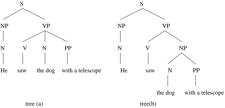
One example of parsing with ambiguity we often see in the literature is to determine the parse of the sentence “He saw the dog with a telescope”. There are at least two possible analyses of the sentence as in Figure (1.1) and the parser needs to determine tree (a) to be the correct parse tree of the sentence. Using
S
NP VP
V NP
N PP
N
saw
the dog He
VP
V N PP
saw the dog with a telescope NP
N
He
with a telescope S
[image:7.612.107.470.56.231.2]tree(b) tree (a)
Figure 1.1: Examples of parsing with ambiguity
In the early stage of statistical parsing, grammar rules of the parser were built by linguists. However, this is a very difficult task due to the complexity of human languages. The grammar rules instead can be projected from the examples of the language. A collection of such examples of correct parses is referred to astreebank
orcorpus.
There are several approaches in statistical parsing. The simplest probabilistic model is Probabilistic Context Free Grammar (PCFG). PCFG was first studied in the late 1960s and early 1970s [Booth & Thompson, 1973]. It is simply a Con-text Free Grammar with probabilities added to the rules, indicating how likely different alternative rewriting rules are. There has been some work on probabilis-tic versions of other grammaprobabilis-tical frameworks such as History Based Grammar [Black et al, 1993], Probabilistic Tree Adjoining Grammar [Resnik, 1992].
1.1
Problem definition
The goal of statistical parsing is to approximate the language’s probability dis-tribution from a treebank as a finite collection of full parse trees. Laplace’s “Principle of Insufficient Reason” attempts to supply a criterion of choice: two events are to be assigned the same probability if there are no reasons to think otherwise. In statistical parsing, the available information of a parse tree is its frequency in the treebank. A statistical parsing model should meet a necessary property of a good learner: whenever one tree appears in the corpus with higher relative frequency than another tree, the model should always assign the former tree higher probability than the latter tree. In chapter 3, we define this property asrank consistent.
In Data-Oriented Parsing, the estimator estimates the underlying STSG from the treebank. Thus the treebank should be considered as a stochastic generating system (to estimate fragments’ weights) as well as a sample of the estimation’s result (the treebank is also a representation of the language). However, in all the existing DOP estimators, the treebank is only used as a stochastic generating system not as a sample for estimating the underlying stochastic grammar. As a result, the outcome probability distribution of the estimations are not consistent with the distributions of trees in the treebank, i.e. they are not rank consistent. The failure to preserve the ranking of full parse trees in the treebank directly relates to other shortcomings of the existing models. [Johnson, 2002] proved that the original DOP model, DOP1, is inconsistent.
1.2
Contribution
This thesis proposes arank consistent DOP estimator where the treebank is not only used as a stochastic generative system but also a sample of the estimated distribution. Perhaps the simplest statistical approach is the DOP maximum likelihood estimation which assigns probabilities to trees in the treebank as their relative frequencies and zero probability to all trees outside the treebank. In term of practicality, assigning all unseen events a zero probability would cause anoverfitting problem which is clearly unsatisfactory.
This thesis also studies the relationship of a rank consistent estimation and a consistent estimation as the training corpus size grows to the limit. The con-sistency is a necessary property in estimation theory. However, the fact that an estimation is consistent or not depends on the choice of the estimation error function.
1.3
Outline
In the following chapter, we introduce the basic concepts of statistical parsing and the Data Oriented Parsing framework. Also, we review the existing DOP models and their shortcomings which were also presented in previous works.
In chapter 3, we discuss the estimation theory’s consistency property in statis-tical parsing. Also, we define the rank consistency property of an estimator and study the relationship between the consistency property and therank consistency
property.
The new estimator, DOPα, is presented in chapter 4. We present how to assign weights to fragments such that their probabilities areproportional to their relative frequencies.
The theoretical property of DOPα is substantiated by the empirical results in chapter 5.
Chapter 2
Background & Notations
In this chapter, the readers first will be made familiar with NLP terminologies and notations that we are going to use throughout the thesis. In section (2.2), the Data-Oriented Parsing framework is introduced with a focus on DOP1 [Bod, 1995]. Also, we review some of other DOP variants and their shortcomings, such as [Buratto, 2003] and [Zollmann, 2004].
2.1
Natural Language Processing Terminologies
and Notations
2.1.1
Terminologies
In formal grammars, words are also referred to as terminal symbols; categories
orconstituent labels such as “NP”, “VP”, . . . , are also referred to asnonterminal
symbols. In the set of non-terminal symbols, there is a distinguished sentence category orstart symbol. The start symbol is often denoted as “S”.
In this thesis, when we mention atree we mean a phrase structure tree where the root and leaf nodes are nonterminal symbols, the leaf nodes can be non-terminal or non-terminal symbols.
A full parse tree is a tree such that its root is the start symbol and all its leaves are terminal symbols.
An utterance or a sentence is a sequence of words. A full parse tree of a sentenceis a full parse tree such that the sequence of its leaves forms the sentence.
S NP N I VP V read NP DT a N book
where “I”, “read”, “a”, “book” are terminal symbols; “S”, “NP”, “VP”, “N”, “V”, “DT” are non-terminal symbols.
Atreebank or acorpus is a sequence of full parse trees. The number of occur-rences of a parse tree in the treebank is significant for the probability estimation that acts on the treebank.
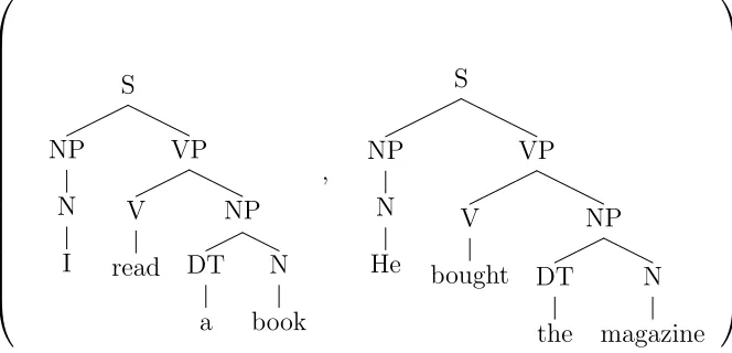
An example of a treebank that consists of the two parse trees of the sentences “I read a book” and “He bought the magazine” is given in Figure (2.1).
[image:11.612.125.457.315.475.2] S NP N I VP V read NP DT a N book , S NP N He VP V bought NP DT the N magazine
Figure 2.1: A treebank example
A probability distribution, PS, over the set S is a function that assigns a
probability to each element in S such that the probabilities of all elements in S
sum up to one.
PS :S→R
X
a∈S
PS(a) = 1
When the setS is clear from the context, we write the probability of an element
a in the set S as P (a).
A language is a probability distribution over a set of full parse trees. If the set of full parse trees is Ω, we denote the language as P∗
An estimator estimates the language from a given treebank. The outcome of an estimation process is a probability distribution over a set of full parse trees. Statistical parsing assumes that the language was generated by a probabilistic grammar. Thus theestimation process actually determines the combination op-erators, the grammar’s rules and the rules’ weights.
2.1.2
Notations
Throughout this thesis, new notations and definitions are introduced whenever needed. However, we present here the most commonly used notations.
LetX be a multi-set and xbe an element of X. We define
• C(X) as the total number of occurrences of all elements in X.
• CX(x) as the number of occurrences ofx inX.
• rfX(x) as the relative frequency of xin X. This means that
rfX (x) = CX(x)
C(X)
Examples: Let tc be a training corpus. C(tc) is the number of full parse trees intc. If t is a full parse tree,Ctc(t) is the number of times t appears in tc.
2.2
Data-Oriented Parsing
As mentioned in the previous chapter, DOP was first introduced in [Scha, 1990]. Later, DOP was formalized by [Bod, 1993]. A DOP model consists of:
• a representation of utterance analyses.
• a definition of fragments, the smallest units used for building new utterance analyses.
• composition operations that define how fragments are combined to new utterance analyses.
• a probabilistic model.
[Hoogweg, 2000] enriched DOP1 with an insertion operation to make the model more robust. [Bonnemaet al., 1999] used the assumption that every derivation
of a tree is equally likely and derived the weights of the fragments based on this assumption. Back-off DOP [Sima’an & Buratto, 2003] considers a derivation of length two of a fragment as a back-off of the fragment. The weights of the frag-ments are discounted to the smaller fragfrag-ments in the derivations of length two in a way that is similar to Katz’s smoothing algorithm. [Zollmann, 2004] presented a consistent DOP estimator using the held-out estimation approach.
In the following sections, we present the DOP framework using its first in-stantiation DOP1 for illustration.
2.2.1
Fragments
DOP captures all the syntactic analyses that appear in the treebank. Each syn-tactic analysis of a tree is represented by a fragment of the tree. A tree f is a
fragment of tree T if
• f consists of more than one node.
• f is a connected sub-graph of T.
• except for the leaf nodes of f, each node in f has the same daughter nodes as the corresponding node in T.
For example, “
S
NP
N
VP
V
read NP
” and “ VP
V NP
” are fragments of the parse
tree “
S
NP
N
I
VP
V
read
NP
DT
a
N
book
”, while “ VP
V
read
” is not a fragment of the tree.
If we extract all fragments of all the trees in the treebank, we get thefragment corpus of the treebank. A fragment corpus is a multi-set of fragments. The fragment corpus of treebank tc is denoted as Fragtc. In DOP, often we are
interested in the fragments with the same root, we denote RFragtc(f) as the
2.2.2
Combination Operator
A combination operator specifies how fragments in the fragment corpus of a treebank are combined to create a new tree. DOP1 has only one combination operator, which is leftmost substitution.
The composition of trees t and u, denoted t◦u, is defined iff the root of tree u is also the leftmost non-terminal leaf of tree t. If t◦u is defined, it yields a copy of treet in which treeuis substituted on the leftmost non-terminal node of tree t.
Example:
S
NP
N
VP
V
read NP
◦ N
I =
S
NP
N
I
VP
V
read NP
and
S
NP
N
VP
V
read NP
◦ NP
DT N
is undefined.
We note that the DOP1 composition operation is not associative, ift, u, v are subtrees then it is not guaranteed that (t◦u)◦v =t◦(u◦v).1
Let t1, t2, . . . , tk be subtrees, t1 ◦t2 ◦. . .◦tk is a shorthand of (. . .((t1 ◦t2)◦
◦t3)◦. . .)◦tk)). . .).
A sequence of subtreesd=ht1, t2, . . . , tkiis aderivation of a full parse treeT if t1◦t2◦. . .◦tk =T
2.2.3
DOP Probability Estimation
The DOP model assigns weights to fragments, and the probability of a tree is calculated on the basic of weights of the tree’s fragments. DOP1 uses the assumption that all fragments are independent; the weight of a fragment is its relative frequency in the treebank’s fragment corpus.
Let tc be a treebank, Fragtc be the treebank’s fragment corpus, f be a
fragment in the fragment corpusFragtc. The weight off according to the DOP1
model is
πdop1(f) =rfRFragtc(f)(f) =
CFragtc(f)
C(RFragtc(f))
where C(RFragtc(f)) is the number of occurrences of all fragments with the
same root as f in Fragtc and CFragtc(f) is the number of f’s occurrences in
Fragtc.
The fragments are considered to be independent, the probability of a deriva-tion is the multiplicaderiva-tion of the weights of fragments involved.
Letd=hf1, f2, . . . fki; the probability of derivation d is:
PDOP1(d) =πdop1(f1)×πdop1(f2)×. . .×πdop1(fk)
LetT be a full parse tree, each derivation of T is a combination of fragments to tree T. Thus the probability of tree T is the sum of the probabilities of its derivations.
Pdop1(T) =
X
dis a derivation ofT
PDOP1(d)
2.2.4
Stochastic Tree Substitution Grammar
The DOP model is based on the Stochastic Tree Substitution Grammar (STSG) formalism [Bod, 1995]. STSG is an extension of Probabilistic Context Free Gram-mar (PCFG) in which the set of rules is a set of elementary trees, which are combined with leftmost substitution composition.
A Stochastic Tree Substitution Grammar G consists of a quintuple G = (VN, VT, S, R, πG)
• VN is a finite set of non-terminal symbols.
• VT is a finite set of terminal symbols; VN ∩VT =∅.
• S is a distinguished non-terminal symbol, called start symbol: S∈VN.
• R is a finite set of elementary trees whose interior nodes are labelled by non-terminal symbols in VN and frontier nodes are labelled by terminal symbols or non-terminal symbols in VN ∪VT.
• πG is a function that assigns elementary probabilities (or weights) to frag-ments in R. It yields positive real values not greater than 1: πG : R → R
where 0< πG(f)≤1 ∀f ∈R.
An STSG partial derivation is a sequence of trees ht1, t2, . . . , tki such that
the result of their composition in that sequence (t1◦t2◦. . .◦tk) is a tree where non-terminal symbols can appear in the leaves.
An STSGderivation is a sequence of trees ht1, t2, . . . , tki such that the result
of their composition in that sequence (t1◦t2 ◦. . .◦tk) is a full parse tree. The
probability of a derivationd=hf1, f2, . . . , fkiis the multiplication of the weights
of the fragments involved.
PG(d) = πG(f1)×πG(f2)×. . .×πG(fk)
The probability of a full parse tree T is the sum of the probabilities of its derivations.
PG(T) = X
dis a derivation ofT
PG(d)
The DOP model uses the assumption that the language is generated by an STSG. The goal of DOP is to determine the STSG from a given treebank. The first DOP model, DOP1, assigns weights to fragments as their relative frequencies in the fragment corpus. Only the DOP estimator in [Hoogweg, 2000] proposed a new insertion operation to the STSG framework, other DOP estimators focus on the weight assignments to fragments in the fragment corpus.
2.2.5
The Shortcomings of DOP1
Bias towards big trees
U
V V V Y w b
a
w w w
Z A
B C
a b
(a) (b)
(c) U X
Y Z
x y
A
U U
[image:16.612.129.451.457.639.2]U
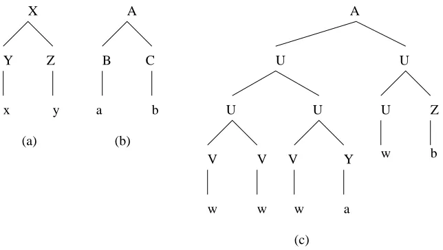
[Bonnema, 2003] used the toy treebank in Figure (2.2) to illustrate DOP1’s bias toward big trees problem.
If we extract all fragments of the treebank we will get 134 different fragments with root “A”. So according to DOP1 estimation, all these fragments are assigned the weight 1/134. There are four different fragments with root “X” so their
weights all are 1/4. It turns out that DOP1 assigns the tree X
Y
a Z
b
a higher
probability than the tree A
B
a C
b
. This contradicts the intuition that the latter
tree which appears in the treebank and should be the preferred parse of the sentence ”ab”.
Let t be a tree root N and t1, t2, . . . , tl are subtrees of t and ti is the subtree
headed by the i-th immediate daughter node of the root node of t. The number of t’s subtrees headed by the root of t, denoted σ(t), is
σ(t) = i=l
Y
i=1
(σ(ti) + 1).
So the number of subtrees of a tree grows exponentially with the tree’s depth. This explains the above counter-intuitive example of DOP1 estimation. In the example, tree (c) with depth four generates 130 fragments with root A, and tree (b) generates 4 fragments with root A, though tree (c) and tree (b) both appear in the corpus once. In DOP1, the big trees contribute high probability mass to fragments of the same root.
Bias & inconsistency
The data in a language can be assumed to follow a “true” probability distribution. An estimator is biased if the difference between the estimator’s expected value 2
and the true distribution is different from zero. The estimator is inconsistent if the estimated distribution does not converge to the true distribution as the size of the training corpus increases.
The bias and inconsistency of DOP1 estimation were first pointed out by [Johnson, 2002]. [Zollmann, 2004] proved that an estimation is biased unless it
2
assigns probability zero to all trees that do not appear in the treebank. DOP1 extracts all fragments from the treebank and generates trees outside the treebank. Hence, DOP1 is biased.
Denote the language as the probability distribution P∗ over the set of full
parse trees Ω. A treebank is a sequence of samples from the set Ω. Let tc be a
treebank with sizen: tc∈Ωn..
An estimator is a function whose input is a treebank and returns a probability distribution of the language. Let est denote an estimator and estn denote the estimator est whose domain is restricted to the treebanks with size n; Mis the set of probability distributions over the set Ω, estn: Ωn→ M.
[Johnson, 2002] defines the difference or the loss function between two prob-ability distributions, P and P∗, by the Euclidean distance metricL(P,P∗)
L(P,P∗) =kP−P∗k2 :=X t∈Ω
P∗(t)(est(tc)(t)−P∗(t))2.
The risk or the estimation error of an estimator est is its expected loss E(L(est(tc),P∗)). The estimator estis inconsistent if
lim n→∞
X
tc∈Ωn
P∗(tc)X
t∈Ω
P∗(t)(est(tc)(t)−P∗(t))2 6= 0 (2.1)
where P∗(tc) is the probability of treebank tc size n in the language P∗. If
tc= (t1, t2, . . . tn) then P∗(tc) = P∗(t
1)×P∗(t2)×. . .×P∗(tn).
To demonstrate the inconsistency of DOP1, [Johnson, 2002] used the example
of a language P∗
Ω where Ω consists of two trees t1 =
S
A
a A
a
and t2 =
S
A
a
with
probability distribution P∗
Ω(t1) =PΩ∗(t2) = 1/2.
A treebank tc of the language P∗
Ω would generate the following fragments
f1 =
S
A
a A
a
, f2 =
S
A
a
A , f3 =
S
A A
a
, f4 =
S
A A ,
f5 =
S
A
a
, f6 =
S
A
, f7 =
A
Further calculation would show that given the treebank tc with size n in-cluding k trees t1 and (n−k) trees t2, DOP1 would assign tree t1 probability
2k/(n+k) and tree t2 probability (n−k)/(n+k). Apply the DOP1 estimation
values to equation (2.1) to get the inconsistency of DOP1.
2.3
Some Variants of DOP Estimators
2.3.1
DOP Maximum Likelihood Estimator
The DOP Maximum Likelihood Estimator (DOPMLE) attempts to generate the
language such that probability of the input treebank is maximized.
Suppose we have the treebank tc, [Bonnema, 2003] shows that DOPMLE
es-timates probability of a tree in the treebank as its relative frequency in the treebank. That means
PDOPMLE(t) = rftc(t) ∀t∈tc
The probability assignment that maximizes the likelihood of tc assigns zero
probability to trees outside the treebank and non-zero to trees in the treebank. DOPMLE probability assignment does not use the treebank as evidence to parse
the sentences outside the treebank. DOPMLE does not allow for generalization,
so it is not applicable in practice.
2.3.2
Bonnema DOP
In [Bonnemaet al., 1999], each full parse tree is considered as a set of all its derivations. Thus, the model views the corpus as the set of all of its derivations, each consisting of a sequence of subtree substitutions. From this different view of the corpus, the model assigns a weight to a fragment based on the fragment’s participation in the set of treebank derivations. We omit here the detailed calcu-lation of weight assignments but present the formula directly:
πBON(f) =
CFragtc(f)
Ctc(root(f))
×2−N(f)
where N(f) is the function that returns the number of internal nodes of fragment f.
Using the 2−N(f) factor, the model reserves a high probability mass for the
However, [Buratto, 2003] reported a disappointing result when the model was tested on the OVIS corpus3. We come back to the motivation of the model that
considers all the derivations of a tree equally likely and independent. In that way, the model looses the dependencies of derivations of a tree. Also, the weight assignment to fragments does not consider the co-occurrence of fragments in a derivation that occurs in the treebank.
2.3.3
Back-off DOP
[Sima’an & Buratto, 2003] developed a different approach to parameter estima-tion for DOP than earlier works.
Each fragment in the fragment corpus is identified as a complex fragment
or an atomic fragment. A fragment f is a complex fragment iff there exist two fragments f1 and f2 such that f1 ◦f2 = f; the derivation hf1, f2i
consti-tutes a backoff of the fragment f. A fragment is atomic iff it has no backoff. [Sima’an & Buratto, 2003] uses the backoff relation between a fragment and a pair of other fragments to form a directed acyclic graph (called backoff graph). A directed edge of the graph points from a node containing fragmentf to another node containing one of its backoff pairs. One fragment might be in the derivations of length two of many other fragments, so one fragment can appear in different nodes of the graph.
The estimation procedure now operates iteratively, top-down over the backoff graph. In the first step, probabilities of fragments are assigned as their rela-tive frequencies. In the subsequent steps, the model redistributes probability mass among DOP fragments by transferring stepwisely probability mass from complex fragments to their backoffs. The redistribution formula is similar to the Katz smoothing method [Sima’an & Buratto, 2003]. The Katz smoothing method helps a system handle the unseen events in then-gram model. Back-off DOP, on the other hand, just adapts the Katz formula to transfer probability mass among fragments. [Zollmann, 2004] gave a review of the model and com-pared the backoff DOP approach and the Katz smoothing method approach.
We believe that the backoff DOP weight assignment reserves higher proba-bility mass for short derivations than for long derivations. By applying back-off between fragments, the model tackles the assumption that derivations are equally likely and independent which is employed by previous models. Also, [Sima’an & Buratto, 2003] reported a very good empirical result when testing on the OVIS corpus.
However, the formula used by [Sima’an & Buratto, 2003] deviates from Katz’s formula. This makes the model problematic (Sima’an, personal communication). When a fragment is a backoff of some other fragments, it will receive probability
mass transferring several times. Intuitively, this situation does not affect the above properties of the model since the transferred probability mass is just a “smoothing” component. The existing work on backoff DOP does not yet provide its mathematical justification.
2.3.4
A Consistent DOP Estimator
[Zollmann, 2004] proposed the first non-trivial consistent DOP (called DOP∗) es-timator using held-out estimation. The training corpus is split into two parts: the extraction corpus (EC corpus) and the held-out corpus (HC corpus). The fragments of the EC corpus is extracted and assigned weights so that the likeli-hood of the held-out corpus is maximized. According to [Zollmann, 2004], this could be achieved by maximizing the joint probability of their shortest deriva-tions. Fragments in EC are assigned weights based on their participation in the shortest derivations of the parse trees in the held-out corpus.
The model first determines punkn: an estimate for the probability that a tree
will be unknown during the testing as the relative frequency of trees in held-out corpus that are not derivable using the fragments of the extraction corpus.
punkn =
CHC({t ∈HC | t is not EC-derivable})
C(HC)
To each fragment f in the treebank’s fragment corpus, the model assigns a weightπdop∗(f):
πdop∗(f) =β(f) +βsmooth(f). (2.2)
Readers are referred to [Zollmann, 2004] to see how the functions β(f) and
βsmooth(f) are derived and their detailed formulas. Here, we are interested in
the following properties of the weight assignment formula:
• β(f)6= 0 if f participates in a shortest derivation of a tree in the held-out corpus.
β(f) = 0 otherwise.
• βsmooth(f) = 0 if punkn = 0 and there are fragments with the same root as
f participating in a shortest derivation of a tree in the held-out corpus. βsmooth(f)6= 0 otherwise.
Thus if punkn 6= 0 then βsmooth(f) 6= 0. So from the weight formula (2.2), it is
clear that when punkn 6= 0, every fragment f in the treebank’s fragment corpus
nonzero weights to a number of fragments that is linear in the number of depth-1 fragments contained in the held-out corpus. This property of DOP∗ is only achieved when punkn = 0. To explain it in another way, the efficiency of DOP∗
is obtained under the condition that every parse tree in the held-out corpus is derivable from fragments in the extraction corpus. In practice, this condition is often fails to be fulfilled because of thesparse data problem: even if the extraction corpus is quite big, the held-out corpus might contain the parse tree of a sentence with unknown words in the extraction corpus.
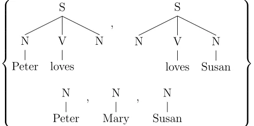
[image:22.612.105.480.236.323.2]Moreover, the efficiency property of DOP∗, when achieved, would bring out another shortcoming of the model: the coverage of DOP∗ is limited in comparison with DOP1. S N Peter V loves N Mary , S N Peter V loves N Susan , S N Mary V loves N Susan
Figure 2.3: A DOP∗ treebank example
Suppose we are given a treebank that contains the parse trees of three sen-tences: “Peter loves Mary”; “Peter loves Susan”; “Mary loves Susan” as in Figure (2.3). S N Peter V loves N , S N V loves N Susan N Peter , N Mary , N Susan
Figure 2.4: The DOP∗ fragments of the treebank example in Figure (2.3)
[image:22.612.161.419.435.563.2]model to parse the sentence. Using the fragments in Figure (2.4), the test sen-tence can not be parsed. However, the sensen-tence is easy to parse using the DOP1 model with the same treebank in Figure (2.3).
[Zollmann, 2004] proved that DOP∗ is consistent. This is a nice property. The DOP∗’s results would improve with the treebank’s size. However, held-out estimation is not a unique approach to get a consistent DOP estimator. According to Sima’an (personal communication), it is possible to devise Back-off DOP’s weight assignments so that consistency is achieved.
We believe that using held-out estimation as [Zollmann, 2004], in the training process the held-out corpus probability is maximized. Also, DOP∗ can be always an efficient DOP estimator if the smoothing component in the weight assign-ment formula, βsmooth(f), only assigns weights to depth-1 fragments (Zollmann,
personal communication). The weakness of the model is the fact that the β(f) component in the weight assignment formula only applies to fragments that par-ticipate in the shortest derivations of the held-out corpus. This would result in a low coverage of the model as explained in the treebank in Figure (2.3). Further calculation of DOP∗’s weight assignment on the treebank in Figure (2.3) would show that the model fails to preserve the frequencies of full parse trees in the treebank.
2.4
Conclusion
We have introduced some NLP terminologies and the notations that we use in this thesis. Also, we introduced the Data-Oriented Parsing framework. The first DOP instantiation, DOP1, achieved state-of-the-art results but has some dis-turbing properties such as bias toward large trees and bias and inconsistency in estimation theory. Bonnema’s DOP model addressed the DOP1’s bias toward big trees problem. Backoff DOP gave a sensible probability estimation to DOP by structuring the set of fragments according to backoff order, tackling the in-dependence assumption of previous work. [Zollmann, 2004] proposed the first consistent DOP estimator using held-out estimation.
DOP estimators use the assumption that the treebank is a representation of an STSG that generates the language. In all the mentioned DOP estimators, the treebank is regarded as a grammar generator. The models do not provide any properties of the estimations’ results on trees in the treebank. For two trees in the treebank, it is possible that the models return a higher probability to the tree that appears with the lower frequency.
provide the definition of arank consistent4 estimator that preserves the ranking
of frequencies in the treebank.
4
Chapter 3
Rank consistent estimation
In this chapter, first we discuss the concept of a consistent estimator in statis-tical parsing in section (3.1). A consistent estimator gives the intuition that the estimator’s error tends to zero as the training corpus grows. There are several definitions of a consistent estimator, the differences between definitions are in how to evaluate the “estimator error”. We show by example that the consistency property of an estimator, however, is dependent on the choice of an “estimator error” function.
In order to help us to decide what is the best estimator to use in any situation, we have to know about the properties of these estimators and choose those which have good properties. The consistency property emphases that the difference between estimator’s result and the true distribution of data in the language should converge to zero as the training corpus size becomes large. However, in practice the treebank is finite and the available data is sparse. The consistency property does not predict the estimator’s performance on finite treebanks. In probabilistic parsing, we would like to place a ranking on possible parses showing how likely each one is, or return the most likely parse of a sentence. So it is important for an estimator to estimate the true ranking probabilities. Section (3.2) will give a formal definition of a rank consistent estimator that preserves the ranking of parse trees’ probabilities. We will show that the original data-oriented parsing model, DOP1, is not a rank consistent estimator.
Also, this chapter studies the relation of a rank consistent estimator and a consistent estimator as the treebank size grows.
3.1
Consistency definition
Let P∗
Ω be the probability distribution of the language over the set of full parse
distribution P for language Ω. In this thesis, we adopt the formal definition of an estimator that appears in [Prescheret al., 2004].
Let estn be an estimator of training corpora of size n and let M be the set of probability distributions over Ω. The estimator estn maps a training corpus of size n to a probability distribution over language Ω as follows:
estn: Ωn→ M tc ∈Ωn ⇒estn(tc) =P ∈ M.
range(estn) is the set of probability distributions that estimator estn returns. Each probability distribution P appears in range(estn) according to the proba-bility of the training corpustc in Ωn that generated P.
Estimator est is a consistent estimator if as n grows to infinity, the probabil-ity distributions in range(estn) approach the true probability distribution P∗ of
language Ω.
An estimator error function Err(estn, P∗) maps the estimator estnand prob-ability distributionP∗ to a non-negative value that measures the difference of set
range(estn) to the true distribution P∗.
Thus estimator est is a consistent estimator if
lim
n→∞Err(estn, P ∗) = 0
There are several ways to define a consistent estimator, and thus there are several ways to define our estimator error function Err.
One approach is to define a loss function L : M × M → R. If P and P0
are two probability distributions then L(P0, P) returns a non-negative real value
that measures the loss of probability distribution P0 with respect to P. The
estimation errorErr(estn, P∗) function takes into account the loss function value
L(P, P∗) of all probability distributions P in range(estn).
For example: A possible definition of estimator error function is
Err(estn, P∗) = max
tc∈ΩnL(estn(tc), P ∗).
[Johnson, 2002] proposes the estimator error (or risk function)
Err(estn, P∗) = X
tc∈Ω
PΩn(tc)× L(estn(tc), P∗)
where the loss function L(P, P∗) is the mean square error of P to P∗ over Ω
L(P, P∗) = X t∈Ω
Another approach is to define estimator error as the probability mass of a set of training corpora for which the loss function value is greater than a real value ε.
Err(estn, P∗) = X
L(estn(tc),P∗)>ε
PΩ∗n(tc)
In [Prescher et al., 2004]L(P, P∗) :=|P −P∗| thus the estimator error
func-tion is:
Err(estn, P∗) = X
|estn(tc)−P∗|>ε
PΩ∗n(tc).
In the following example, an estimator est and two estimation error functions Err1 and Err2 are given. We will show that estimator est is consistent when
estimator error function Err1 is chosen and it is not consistent when Err2 is
chosen.
Example 3.1.1 We define Err1(estn, P∗) as in [Johnson, 2002]
L1(P∗,estn(tc))(t) = (estn(tc)(t)−P∗(t))2
L1(P∗,estn(tc)) =
X
t∈Ω
P∗(t)(estn(tc)(t)−P∗(t))2
Err1(estn, P∗) =
X
tc∈Ωn
P∗(tc)X t∈Ω
P∗(t)(estn(tc)(t)−P∗(t))2
Estimator error function Err2:
If we consider the loss value of probability distribution P0 w.r.t probability
distributionP as the total probabilities of trees for which probability distribution P0 is different than probability distribution P, then the loss function L
2(P0, P)
is defined as follows:
L2(P∗,estn(tc))(t) =
0 if P∗(t) = estn(tc)(t)
1 if P∗(t)6= est
n(tc)(t)
=⇒ L2(P∗,estn(tc)) =
X
t∈Ω
P∗(t)L2(P∗,estn(tc))(t)
Err2(estn, P∗) =
X
tc∈Ωn
P∗(tc)L2(estn(tc), P∗)
Let Ω be a set of two trees Ω ={t1, t2}and the languagePΩ∗ with distribution:
P∗
Lettc be a training corpus size n of Ωn, estimator estn is defined as follows:
estn(tc)(t1) =
1 2−
1
n estn(tc)(t2) = 1 2+
1 n .
i) Examine the consistency property of est when the estimation error func-tion isErr1
L1(estn(tc), P∗)(t1) = (estn(tc)(t1)−P∗(t1))2 = (
1 2 − 1 n − 1 2)
2 = 1
n2
L1(estn(tc), P∗)(t2) = (estn(tc)(t2)−P∗(t2))2 = (
1 2 + 1 n − 1 2)
2 = 1
n2
L1(estn(tc), P∗) =P∗(t1)L1(estn(tc), P∗)(t1) +P∗(t2)L1(estn(tc), P∗)(t2)
L1(estn(tc), P∗) = 1 2n2 +
1 2n2 =
1 n2
⇒Err1(estn, P∗) =
X
tc∈Ωn
P∗(tc)X t∈Ω
P∗(t)L1(estn(tc), P∗)(t)
| {z }
=1/n2
= X
tc∈Ωn
P∗(tc) 1 n2
= 1
n2
X
tc∈Ωn
P∗(tc) = 1
n2
⇒ lim
n→∞Err1(estn, P
∗) = lim
n→∞
1 n2 = 0.
So est is consistent with estimation error function Err1.
ii) Examine the consistency property of est when the estimation error function is Err2.
Because ∀n: estn(tc)(t1)6=P∗(t
1) and estn(tc)(t2)6=P∗(t2) so:
∀n : L2(estn(tc), P∗)(t1) =L2(estn(tc), P∗)(t2) = 1
⇒Err2(estn, P∗) =
X
tc∈Ωn
P∗(tc)X t∈Ω
P∗(t)L2(estn(tc), P∗)(t)
| {z }
=1
= X
tc∈Ωn
P∗(tc)X t∈Ω
P∗(t) = 1
⇒ lim
n→∞Err2(estn, P
∗) = lim
n→∞1 = 16= 0.
As the training corpus grows to the limit, a consistent estimator’s error tends to zero. Though the consistency property of an estimator is intuitively appealing, the above discussion shows that whether an estimator is consistent or not depends on the definition of estimator error. In this thesis, we use the estimator error defined by [Johnson, 2002], unless it is explicitly stated otherwise.
The consistency property of an estimator expresses the estimator’s results when the training corpus size grows to infinity. In practice, the training corpus is always a finite sequence of trees. Consistency does not give us information about the estimator when the training corpus size is finite. In the next section, we introduce the property ofrank consistency which means that given a training corpus, the estimator’s result is always consistent with the ranking frequency of trees in the training corpus.
3.2
Definition of Rank Consistent Estimator
Let s be a sentence; the parser evaluates the probability of a tree t to be the parse ofs by findingP(t|s). Tree t∗ is the parse of s if
t∗ = arg max
t P(t|s) = arg maxt
P(t, s)
P(s) = arg maxt P(t, s)
Given tree t, sentence s is always determined, thus finding probability P(t, s) is equivalent to finding probability of the tree, P(t).
The estimator should assign probabilities to all trees in the language using a finite treebank as the language’s partial evidence. The most famous criterion for choosing probabilities is Laplace’s Principle of Insufficient Reason (or Indif-ference Principle) [Guiasu & Shenitzer, 1998]: when one has no information to distinguish the probabilities of two events the best strategy is to consider them equally likely. Applying Laplace’s Principle, the estimator should find a proba-bility assignment that agrees with the information in the treebank. One crucial constraint is that when two full parse trees appear in the treebank with the same frequency the estimator should always assign them the same probability. Also, when one tree appears in the treebank with a higher frequency than another tree, it should be assigned a higher probability than the other tree.
Let Ω be the language with probability distribution P∗; let est(tc) be the
estimator induced by training corpus tc. The estimator est(tc) will give the
correct most probable parse of a sentence or a correct priority of trees to be the parse of the sentence if for any tree t1 and t2 of the language Ω
P∗(t1)≤P∗(t2) implies est(tc)(t1)≤est(tc)(t2).
Let t1 and t2 be two trees in training corpus tc, we have P∗(t1) ≤ P∗(t2)
We define the concept ofrank consistency that adopts the mentioned ranking preservation property.
Definition 3.2.1 An estimator est is rank consistent if for any training corpus
tc, if treet1 and treet2 are in corpustcwith frequencyCtc(t1) andCtc(t2)
re-spectively, the estimator est induced bytcwill assign treet1a greater probability
than t2 if Ctc(t1) is greater than Ctc(t2) and vice versa.
Contemplation
The rank consistency is a necessary property of an estimation. It guarantees that the estimation preserves the trees’ frequencies in the treebank. The rank consistent estimator should assign its probability in such a way that the unknown tree’s probability is an adaption of the probabilities of other similar trees that appear in the treebank.
If we assume that the unknown tree is built up from fragments that appear in the treebank as in DOP framework, the estimator should not only preserve the ranking consistency of full parse trees but also preserve the ranking consistency of fragments that appear in the treebank.
3.2.1
The failure of DOP1
In DOP1, [Bod, 1995] defines the weight of a fragment t of category X as its frequency in the tree bank divided by the frequency of all subtrees with the same categoryX.
In this section, we show that DOP1 is notrank consistent where the selection criterion is most probable parse or most probable derivation.
DOP1 most probable parse is not rank consistent
[Johnson, 2002] proved that DOP1’s most probable parse is not consistent and biased. We will show that it is notrank consistent either.
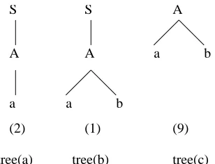
We take as an example the tree bank as given in Figure (3.1), where tree (a) appears two times in the corpus, tree (b) appears once and tree (c) appears nine times. Rank consistency requires that tree (a), which appears twice, should be assigned a higher parse tree probability than tree (b), which appears once in the corpus. This tree bank will generate the corpus fragments as shown in Figure (3.2). The numbers in brackets under fragments indicate their DOP1 weights.
tree(a) tree(b) tree(c) S
A
a
S
A
A
a b
a b
[image:31.612.213.367.71.189.2](2) (1) (9)
Figure 3.1: Example tree bank
a A
S
A
A
a b
a b
(1/6) (10/12) S
a A
A S
(3/6)
(2/6)
[image:31.612.172.408.263.369.2](2/12)
Figure 3.2: Fragments of tree bank in figure 3.1
S
A
a
S
A
a b
S
A
a b
S
A
a
f( )= 2 > f( )=1
P ( )=15/36 < P ( )=21/36 DOP1
DOP1
[image:31.612.183.392.442.625.2]tree probabilities as depicted in Figure (3.3). DOP1 assigns tree (a) a lower parse tree probability than tree (b). Thus, when calculating the most probable parse of a tree, DOP1 does not give the result consistent with trees’ frequencies. Hence, DOP1 is notrank consistent.
DOP1 most probable derivation is not rank consistent
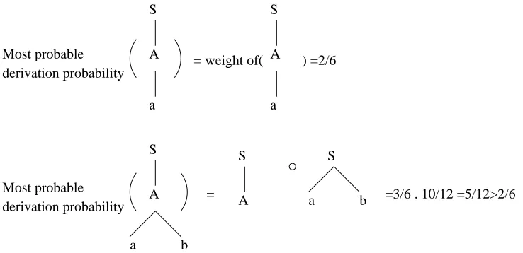
A derivation probability is calculated as product of its fragments’ weights. In DOP1 a fragment’s weight is its relative frequency. If two trees appear in the corpus, these two trees are also in fragment corpus. It would be expected that DOP1’s most probable derivation probabilities would be their weights in the frag-ment corpus. However, this is not always true. If one tree appears in the corpus with low frequency and its subtrees appear in the corpus with high frequencies, a derivation that involves more fragments may be the DOP1 ’s most probable derivation. Thus DOP1’s most probable derivation is not consistent with the tree’s low frequency in the corpus and it is notrank consistent.
We use the tree bank in Figure (3.1) again as an example. From the
fragments’ weights in Figure (3.2) we have the most probable derivation of two trees as depicted in Figure (3.4). DOP1 most probable derivation as-signs tree S,(A,(a,()),(b,()))) higher probability than tree S,(A,(a,())) though S,(A,(a,()),(b,()))) has lower frequency in the tree bank than S,(A,(a,())). So DOP1 most probable derivation is notrank consistent.
Most probable derivation probability
S
A
a
S
A
a
S
A
a b
Most probable derivation probability
= weight of( ) =2/6
S S
A a b
[image:32.612.102.471.395.574.2]= =3/6 . 10/12 =5/12>2/6
3.2.2
A
rank consistent
estimator versus a consistent
es-timator
Consistency and rank consistency are two different properties of estimators. A rank consistent estimator estimates the probabilities of trees in the corpus the same ranking as their frequencies. It uses the assumption that the ranking of trees’ frequencies in the corpus is also the ranking of trees’ probabilities in the language. This assumption is quite reasonable because the training corpus is the only data that the estimator observes from the language. The consistency definition considers the estimator’s result from all the possible training corpora. In this section, we study if a consistent estimation preserves the ranking of tree probabilities as their relative frequencies in the corpus.
We give an example to show that when the training corpus grows to infinity, a consistent estimator is not arank consistent estimator.
However, for any two trees with different probabilities in the language, the total probability of training corpora such that a consistent estimator yields an inconsistent ranking to these trees tends to zero.
In the limit a consistent estimator is not guaranteed to be rank con-sistent
We use again the estimator est in example (3.1.1).
Let Ω ={t1, t2} and PΩ∗(t1) =PΩ∗(t2) = 12
tc is a training corpus sized n of Ω, estimator estn is defined as follows:
estn(tc)(t1) =
1 2−
1
n estn(tc)(t2) = 1 2+
1 n.
Example (3.1.1) shows that estimator est is consistent when the mean-square error is used as estimator error function. However, estimator est always selects the tree t2 as a more probable tree than tree t1. Now we prove that est is not
rank consistent.
Let Ctc(t1) and Ctc(t2) be the frequencies of t1 and t2 in training corpus
tc. The probability of a training corpus tc size n is:
P∗(tc) = (P∗(t1))Ctc(t1)(P∗(t2))Ctc(t2)
= (1 2)
Ctc(t1)(1
2)
Ctc(t2) = (1
2)
Ctc(t1)+Ctc(t2) = (1
2) n.
Estimator est estimates probability of t1 less than t2. So if in training corpus
tcfrequency of treet1 is equal or greater than frequency of tree t2, the estimator
Because each training corpus tc of size n has the same probability 1/2n, the total probabilities of training corpora in which the frequency of tree t1 is equal
or greater than the frequency of tree t2 is at least 1/2 or total probabilities of
training corpora size n that the estimator est estimates trees’ probabilities not consistent with trees’ frequencies is at least 1/2 for all n.
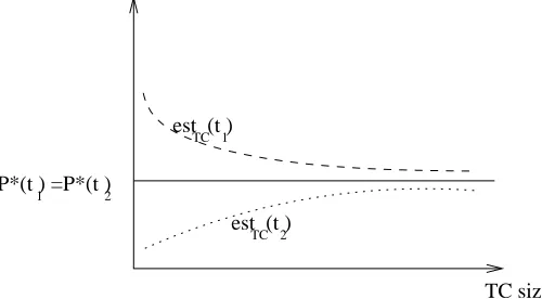
Estimator est and language Ω above are examples of a language in which there are two trees with the same true distribution while estimator est, though consistent, always give the probability of one tree different than the other tree. This situation is depicted in the graph of Figure(3.5)
P*(t ) =P*(t ) 1 2
TC size est (t )
est (t ) TC
TC 1
[image:34.612.161.411.211.349.2]2
Figure 3.5: A consistent estimator est and most probable derivation of two trees in the corpus
For any tree in the language, the difference between a consistent estimator’s result and tree’s actual distribution approaches zero as the training corpus size grows to infinity. However, this property of a consistent estimator does not imply that in the limit the estimator estimates probabilities trees in the corpus consistent with their actual ranking or their relative frequency in the corpus.
In the previous section, we showed that a consistent estimator does not pre-serve the ranking of relative frequencies of all trees in the corpus. However, for any two treest1 and t2 with different probabilities in the language, we will prove
that the consistent estimator estimates their probabilities consistent with their relative frequencies when the corpus size grows to infinity.
The intuition above is stated formally by the following theorem (3.2.2). Given corpus tc, a consistent estimator est estimates tree t1 and t2
prob-abilities estn(tc)(t1) and estn(tc)(t2) consistent with ranking of their relative
frequenciesrftc(t1) andrftc(t2) if
Theorem 3.2.2 Let t1 and t2 be two trees in language Ω with different
proba-bilities. If est is a consistent estimator of Ω, then for all q > 0 there exists an integer N that
X
(estn(tc)(t1)−estn(tc)(t2))(rftc(t1)−rftc(t2))<0
P∗(tc)< q ∀n > N
To prove theorem (3.2.2) we need the following lemma:
Lemma 3.2.3 Let Ω be language with true distribution P∗, est be a consistent
estimator. For all treest0 of Ω and for any real value ε >0, q >0 there exists N
such that
X
|estn(tc)(t0)−P∗(t0)|>ε
P∗(tc)< q ∀n > N
Proof: Because est is a consistent estimator so∀q0 >0, there existsN such that
X
tc∈Ωn
P∗(tc)X t∈Ω
P∗(t)(P∗(t)−estn(tc)(t))2 < q0 ∀n > N (3.2)
Choose q0 =q.P∗(t
0).ε2 and replace to (3.2):
X
tc∈Ωn
P∗(tc)X t∈Ω
P∗(t)(P∗(t)−estn(tc)(t))2 < q.P∗(t0).ε2 (3.3)
Applying
P∗(t0)(P∗(t0)−estn(tc)(t0))2 <
X
t∈Ω
P∗(t)(P∗(t)−estn(tc)(t))2
to (3.3). We have
X
tc∈Ωn
P∗(tc)P∗(t0)(P∗(t0)−estn(tc)(t0))2 < q.P∗(t0).ε2 (3.4)
Applying
X
tc∈Ωn,|est
n(tc)(t0)−P∗(t0)|>ε
P∗(tc)< X
tc∈Ωn
P∗(tc)
to (3.4) we have:
X
tc∈Ωn,|est
n(tc)(t0)−P∗(t0)|>ε
P∗(tc)P∗(t0) (P∗(t0)−estn(tc)(t0))2
| {z }
>ε2
(3.5)
⇒ X
tc∈Ωn,|est
n(tc)(t0)−P∗(t0)|>ε
P∗(tc)P∗(t0).ε2 < q.P∗(t0).ε2. (3.6)
⇒ X
tc∈Ωn,|estn(tc)(t
0)−P∗(t0)|>ε
P∗(tc)< q (3.7)
qed
Note [Zollmann, 2004] proposes a definition of strong consistent estimation. According to him, an estimation is strongly consistent if thesupremumdifference of the estimation result and the true distribution in the whole language con-verges to zero as the training corpus grows large. Then in (theorem (3.1.1), [Zollmann, 2004]), he proved that a strong consistent estimation is also a John-son consistent estimator. The remaining question goes in the opposite direction of his theorem: whether a consistent estimation is also a strong consistent esti-mation? In our lemma (3.2.3), we solve a somewhat weaker form of the question. Given any tree t0, in the limit a consistent estimation will converge on its true
probability. The lemma serves as the main step in the proof of theorem 3.2.2.
Proof of 3.2.2. We use lemma (3.2.3) to prove theorem (3.2.2) as follows:
Choose ε= 1 2|P
∗(t
1)−P∗(t2)|, because P∗(t1)6=P∗(t2) so ε >0.
Suppose P∗(t
1)< P∗(t2) and
|estn(tc)(t1)−P∗(t1)|< ε and |estn(tc)(t2)−P∗(t2)|< ε
⇒estn(tc)(t1)< estn(tc)(t2) (3.8)
Similarly, if
|rftc(t1)−P∗(t1)|< ε and |rftc(t2)−P∗(t2)|< ε
⇒rftc(t1)<rftc(t1) (3.9)
From (3.8) and (3.9) we have
So if (estn(tc)(t1)−estn(tc)(t2))(rftc(t1)−rftc(t2))<0, then
|estn(tc)(t1)−P∗(t1)|> ε or |rftc(t1)−P∗(t1)|> ε
or |estn(tc)(t2)−P∗(t2)|> ε or |rftc(t2)−P∗(t2)|> ε
where ε = 1
2|P
∗(t
1)−P∗(t2)|
(3.10)
Choose q0 = q
4
est is a consistent estimator, apply lemma (3.2.3): there exists Nest1 >0,
Nest2 >0 that
X
tc∈Ωn,|est
n(tc)(t1)−P∗(t1)|>ε
P∗(tc)< q0 ∀n > Nest1
and
X
tc∈Ωn,|est
n(tc)(t2)−P∗(t2)|>ε
P∗(tc)< q0 ∀n > Nest2
Relative frequency estimator (DOPMLE) is also a consistent estimator, apply
lemma (3.2.3): there exists NMLE1 >0 and NMLE2 >0 that
X
tc∈Ωn,|rf(tc)(t
1)−P∗(t1)|>ε
P∗(tc)< q0 ∀n > NMLE1
X
tc∈Ωn,|rf(tc)(t
2)−P∗(t2)|>ε
P∗(tc)< q0 ∀n > NMLE2
Choose N = max{Nest1, Nest2, NMLE1, NMLE2}, we have
X
tc∈Ωn,|est
n(tc)(t1)−P∗(t1)|>ε
P∗(tc)< q0 ∀n > N (3.11)
X
tc∈Ωn,|rf
tc(t1)−P∗(t1)|>ε
P∗(tc)< q0 ∀n > N (3.12)
X
tc∈Ωn,|est
n(tc)(t2)−P∗(t2)|>ε
X
tc∈Ωn,|rf
tc(t2)−P∗(t2)|>ε
P∗(tc)< q0 ∀n > N (3.14)
Sum over (3.11), (3.12), (3.13) and (3.14):
X
tc∈Ωn,|est
n(tc)(t1)−P∗(t1)|>ε
P∗(tc) + X
tc∈Ωn,|rf
tc(t1)−P∗(t1)|>ε
P∗(tc) +
X
tc∈Ωn,|est
n(tc)(t2)−P∗(t2)|>ε
P∗(tc) + X
tc∈Ωn,|rf
tc(t2)−P∗(t2)|>ε
P∗(tc) <
q0+q0+q0 +q0 =q ∀n > N
⇒ X
tc∈Ωn,|est
n(tc)(t1)−P∗(t1)| >ε
or |rftc(t1)−P∗(t1)| >ε
or |estn(tc)(t2)−P∗(t2)| >ε
or |rftc(t2)−P∗(t2)| >ε
P∗(tc)< q ∀n > N (3.15)
Apply result in (3.10) to (3.15) we have
X
(estn(tc)(t1)−estn(tc)(t2))(rftc(t1)−rftc(t2))<0
P∗(tc)< q ∀n > N
qed
3.3
Conclusion
We have discussed the consistency property of probability estimation in Natural Language Processing. A consistent estimator gives the intuition of an estimator assigning true probabilities for trees as their true probability in the language when the training corpus grows to infinity. We show by example that the consistency property of an estimator depends on the definition of error function.
The training corpus is the only evidence of the language for an estimator. If one tree appears with higher frequency than the other tree in a training corpus, intuitively the former tree has higher probability in the language. We defined this estimation’s property asrank consistent and proved that the commonly used DOP1 is notrank consistent.
any two trees with different actual probabilities in the language, in the limit a consistent estimator estimates their probabilities consistent with their frequencies in the tree bank.
Chapter 4
The new DOP estimation -
DOP
α
4.1
Overview
For estimation, a treebank serves as the only evidence of the language, thus the distribution in the treebank is assumed to reflect the true distribution. The purpose of estimation is to approximate this true distribution of the language from the treebank. In the previous chapters, we discuss the rank consistency property that the ranking of parse tree probabilities of trees in the treebank consistent with their frequencies. In this chapter, we will present a rank consistent DOP estimator.
The DOP estimations assume that trees of the language are generated by an STSG that is encoded in the treebank. Thus in arank consistent DOP estimation, the treebank should be regarded not only as a stochastic generating system but also as a sample of the stochastic process.
A naive solution for the DOP model, DOPMLE, assigns probabilities to trees in
the corpus as their relative frequencies and zero probability for the trees outside the corpus. However, the treebank is finite and just contains a portion of the language. The DOPMLE is extremely overfitting and against the DOP spirit that
a new sentence is parsed by combining the syntactic analyses that already appear in the treebank.
the ranking of the fragments is also rank consistent.
Now we discuss the roles of extracted fragments and their weights in the DOP estimation process. If we retrieve only depth-one fragments from the treebank, the resulting PCFG model also generates all the trees and subtrees that DOP generates. However, the PCFG model does not account for the co-occurrence of rules. In DOP, all the fragments of the treebank are extracted. This makes DOP able to capture all the long distance dependencies of the constituents, related lexical items and structures that appear in the treebank.
NP
a
DT N
book
NP
the
DT N
NP
the
DT N
magazine book
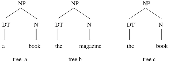
[image:41.612.144.434.185.290.2]tree a tree b tree c
Figure 4.1: Tree (a) and (b) are fragments of the corpus that contains two sen-tences “I read a book” and “He bought the magazine” while tree (c) is not a fragment of the corpus. All three trees can be derived from smaller fragments of the corpus.
Let us consider the toy treebank in Figure (2.1) that contains the parse trees of two sentences “I read a book” and “He bought the magazine”. Tree (a) and tree (b) in Figure (4.1) are fragments of the treebank’s fragment corpus with relative frequencies 0.1 and 0.1 respectively while tree (c) is not a fragment of the treebank. However, all trees (a), (b) and (c) can be generated from their smaller subtrees in the fragment corpus. In DOP, fragments (a), (b) are included in the STSG rules to account for the co-occurrence of their sub-structures in the corpus. Thus the estimation should also assign weights to fragments in such a way that the joint dependency of the fragment’s subtrees are recovered. The dependency of a fragment’s sub-structures is captured by the fragment’s relative frequency in the fragment corpus that DOP extracts from the treebank.
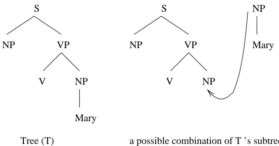
Suppose the STSG G = (VN, VT, S, R, π) generates the language. The STSG grammar treats fragments as if they were disjoint. The dependencies of sub-structures in a tree are recovered by summing up over all the derivations of the tree. Let T be a full parse tree of grammar G. A derivation of T represents a possible combination of fragments in G. Also, a derivation of T is one possible way of generating T from grammar G. The parse tree probability of T, PG(T), is the sum of all the derivations’ probabilities of T.
The STSG model G not only generates full parse trees, it also generates
symbol of the grammar. However, the existing STSG definitions of derivation and parse tree probability are only applicable to full parse trees. As we will explain in section (4.2), the STSG partial derivation concept fails to capture all the possible combinations of fragments to a tree. To support the new view of the corpus as its collection of fragments, the STSG derivation definition is generalized so that it is applicable to an arbitrary tree. We call itderivation∗. Aderivation∗ of tree
t, according to grammarGis a possible combination of fragments in G to treet. The formal definition ofderivation∗ is given in section (4.2). We define the parse
probability of t, PG(t), is the sum of all derivations∗ probabilities. It specifies
how likely t is generated from grammar G and also captures the dependencies of sub-structures in t. For a full parse tree, the new notions of derivation∗ and
probability coincide with the original definition of derivation and full parse tree probability.
From the above discussion, we see the co-occurrences of subtrees from the treebank’s point of view and from the STSG’s point of view. From the treebank’s point of view, the co-occurrences of a tree’s sub-structures is captured by the tree’s relative frequency in the treebank’s fragment corpus. From the STSG point of view, the co-occurrences of a tree’s sub-structures are captured by the parse probability of the tree. So how should the estimator assign weights to fragments such that their probabilities reflect their relative frequencies in the fragment corpus and also the model is rank consistent?
One answer would be an imaginary estimator γ that assigns weights to frag-ments such that Pγ(f) =rfRFrag(f) for all fragmentsf in the fragment corpus Fragtc.1 However, this condition is too strict: There are corpora of a language
such that this condition can not be fulfilled. For example, if we have the tree-bank in Figure (4.2) and its fragment corpus is in Figure (4.3), we cannot assign weights to its fragments that fulfill the condition Pγ(f) = rfRFrag(f).
To fulfill the condition Pγ(f) = rfRFrag(f), the weight of S
A
a b
is calculated
1
tree(a) tree(b) tree(c) S
A
a
S
A
A
a b
a b
[image:43.612.212.366.127.252.2](2) (1) (9)
Figure 4.2: A treebank example
a A
S
A
A
a b
a b
(1/6) (10/12) S
a A
A S
(3/6)
(2/6)
(2/12)
[image:43.612.170.407.444.548.2]from its parse tree probability as follows: Pγ S A a b
=πγ( S
A
)×πγ( A
a b
) +πγ( S A a b ) (4.1) Because πγ( S A
) = Pγ
S
A
=rfRFrag S A πγ( A a b
) = Pγ
A
a b
=rfRFrag A a b .
Apply the above equations to (4.1), we have
⇒rfRFrag
S A a b
=rfRFrag
S
A
×rfRFrag
A
a b
+πγ(
S A a b ) ⇒ 2 6 = 3 6 × 10 12 +πγ(
S A a b ) ⇒πγ( S A a b
) = 2
6 −
5 12 <0.
So it is impossible to assign weights to fragments to fulfill the constraint Pγ(f) =rfRFrag(f) for all fragments f.