Epiphytic bryophytes and habitat microclimate variation in lower montane rainforest, Peru

(1)

Epiphytic bryophytes and habitat

microclimate variation in lower montane

rainforest, Peru.

by

Jerry Romanski BSc.

(University of Tasmania)

(2)

Declaration

This thesis contains no material which has been accepted for the award of any other degree or diploma in any tertiary institution, and to the best of my knowledge and belief, contains no material previously published or written by another person, except where due reference is made in the text of the thesis.

Signed

Jerry Romanski BSc. Signed

Jerry Romanski

(3)

Abstract

A survey of epiphytic bryophytes and a study of microclimatic variation within a tree

crown were conducted in lower montane rainforest at 2400 m in the Peruvian Yungas. A

total of 129 species (87 hepatics, 1 hornwort and 41 mosses) were collected on 3 trees,

using different methodologies. A single Weinmannia sp. host supported 110 species (77

hepatics, 1 hornwort and 32 mosses). Species with a wide distribution on the hosts made

up 47% of the epiphytic assemblage, 22% were limited to the trunks and 31% occurred

only in the crowns. The overall hepatic to moss ratio was 2.15:1. Mosses exhibited a

narrower distributional range than hepatics. The greatest species richness and abundance

was found on the large branches in the mid-crown. Species found in the mid-crown

generally had a broader distribution on hosts than those found on the lower trunk or the

outer crown. Classification and ordination analyses of the species and environmental data

indicated the presence of 4 communities: an outer crown, a mid to mid-outer crown, an

upper trunk and a lower trunk community. Species distribution on hosts in the present

study appeared to be influenced by the intensity of radiation, particularly diffuse radiation,

and relative humidity related to a moisture availability gradient. Temperature appeared

least important. Six species were selected as potential microclimate change indicators.

Variation in temperature, relative humidity, visible sky fraction, leaf area index and

radiation intensity were measured throughout a single canopy a co-dominant Weinmannia

sp. The opposing gradients of temperature and relative humidity displayed similar

fluctuation patterns as found in lowland rainforest, although the range of the gradients was

smaller, possibly due to greater atmospheric mixing facilitated by the more permeable

canopy at the montane rainforest study site. Microclimate stability decreased with

distance above the ground. The lower trunk micro-habitat was the most humid, coolest

and least illuminated. The highest temperature and lowest relative humidity were

recorded in the mid-outer crown, closely followed by the most irradiated crown periphery.

(4)

radiative cooling in the evening. The air above the canopy was warmer at night than any

micro-habitat on the tree host.

The study found 27 bryophytes species (5 mosses, 22 hepatics) not previously recorded for

Peru. Recommendations for methodology in future bryophyte surveys in Peruvian lower

montane rainforest are presented. Future studies must parallel more concerted efforts to

raise the awareness of the local population about the ecological importance of bryophytes,

particularly in cloud forests.

Resumen

Un estudio de briofitas epifitas y de la variación microclimática dentro de la copa de un

árbol fueron conducidos en los bosques mas bajos de montaña a 2400 m. en las Yungas

peruanas. Un total de 129 especies (87 hepáticas, 1 antocerota y 41 musgos) fueron

recolectadas en 3 árboles, usando diferentes metodologías. En un solo Weinmannia sp. se

encontró 110 especies (77 hepáticas, 1 antocerota y 32 musgos). Especies con una amplia

distribución en los árboles contribuyeron 47% de epifitas, 22% fueron limitados a los

troncos y 31% ocurrieron solo en las copas. La totalidad de tasa de hepáticas a musgos fue

2.15:1. Los musgos mostraron un rango de distribución mas estrecho que las hepáticas.

La más grande riqueza y abundancia de especies fue encontrada en las ramas grandes de la

media copa. Las especies encontradas en la media copa generalmente tuvieron una

distribución mas ancha en los árboles que aquellos encontrados en el tronco bajo o en la

copa exterior. Los análisis de clasificación y ordenación de las especies y data de medio

ambiente indicaron la presencia de 4 comunidades: Copa exterior, de media copa a media

copa exterior, parte superior del tronco y la comunidad de la parte baja del tronco. La

distribución en los árboles del presente estudio pareció ser influenciada por la intensidad

de radiación, particularmente radiación difusa y relativa humedad relacionada a la escala

de disponibilidad de agua. La temperatura pareció menos importante. Seis especies

(5)

La variación de la temperatura, humedad relativa, fracción visible de cielo, índice de la

área foliar e intensidad de radiación fueron medidos en todas partes de un co-dominante

Weinmannia sp. Las escalas opuestas de temperatura y humedad relativa mostraron

similar fluctuación como los encontrados en Selva Baja; sin embargo, el rango de las

escalas fue más pequeño, posiblemente a causa de mejor combinación atmosférica

facilitada por el dosel más abierto en bosque de montaña elegido para el presente estudio.

La estabilidad microclimática disminuyo con la distancia del suelo. El micro hábitat en la

parte baja del tronco fue el más húmedo, más fresco y menos iluminado. La temperatura

más alta y humedad relativa mas baja fueron registradas en la media copa exterior,

cercanamente seguido por la periferia de la copa mas irradiada. La temperatura sobre el

dosel permaneció más fresco durante el día que la misma copa del árbol. El promedio de

horario de la temperatura mas bajo fue registrado en la media copa, causado por el rápido

enfriamiento radiativo en la noche. El aire sobre el dosel fue mas caliente en la noche

como en cualquier micro-hábitat en el árbol.

En el estudio se encontró 27 especies de briofitas (5 musgos, 22 hepáticas) que no eran

citados en el Perú. Las recomendaciones para metodología en estudios futuros de briofitas

en los bosques de montaña baja peruana, son incluidas en el presente informe. Futuros

estudios deben suceder paralelos a los esfuerzos concertados para la concientización de la

población sobre la importancia ecológica de las briofitas, particularmente en los bosques

(6)

Acknowledgments

This project would not have become reality without the assistance and support of many, both in Tasmania and Peru. This unusual honours project was made possible by the overwhelming support and encouragement of Professor Jamie Kirkpatrick and Dr. Emma Pharo at the School of Geography and Environmental Studies, University of Tasmania.

The present study was inspired by Damien Catchpole and his study of vascular epiphytes in a Ficus sp. on the slopes of the Yanachaga-Chemillén Range, Peru. He provided much advice and facilitated many aspects of the study and home life in Oxapampa. Also, a thank you to Karen Richards, whose love of nature has always been and will continue to be an inspiration.

Much logistical support was provided by the Instituto Nacional de Recursos Naturales (INRENA). Co-operation of the staff at the Oxapampa office headed by Eduardo De la Cadena is much appreciated. Access to the facilities of the Missouri Botanical Garden Selva Central branch was invaluable. The staff, particularly Rodolfo Vasquez Martinez, his partner Rocio Rojas and Abel Monteagudo made me feel very welcome. I would also like to thank Percy Summers at Pro-Pachitea and the Fundación Peruana para la Conservación de la Naturaleza (Pro-Naturaleza) for their logistical support. A special thanks to Assoc. Prof Carlos Llerena Pinto who assisted with student visa requirements.

The volume of taxonomic literature that was necessary to complete the present study is staggering. Majority of it had to arrive in electronic format to this corner of the Amazon basin. I would like to thank the University and the library and document delivery staff, for their assistance. Prof. Rob Gradstein provided some key literature, as did Rod Seppelt, who also donated his time to demonstrate some laboratory techniques.

Bryologist are rare anywhere and especially so in Peru. A special thank you to Jasmin Opisso Mejia at the Museo de la Historia Natural in Lima, who gave up much time and provided the expertise necessary to clarify many doubts and verify the moss identifications.

(7)

List of figures

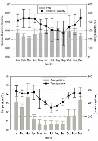
Fig. 1. Lower montane rainforest near the study site “El Cedro” at 2400 m………..…21 Fig. 2. Mean monthly relative humidity, photosynthetically active radiation

(PAR), precipitation and temperature at “El Cedro”, Yanachaga-

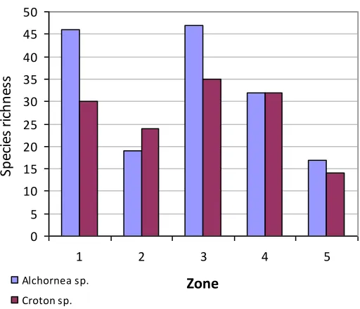
Chemillén National Park, Peru………..22 Fig. 3. Zone species richness in the Alchornea sp. and Croton sp. hosts………....27 Fig. 4 A) Alchornea sp. zone 1 species rarefaction as proportion of species from

a known population; B) zone 4 species rarefaction curve (pooled data

from Alchornea sp. and Croton sp. individuals)………...…..28 Fig. 5 Plot of rank of observed species in 5 Johansson zones (sample area of

0.06 m2_{) and proportion of observed species captured in 0.03 m}2_{in each}

zone……….29 Fig. 6 Stratification of the trunk and crown following Johansson (1974), looking

south………33 Fig. 7 Shielded LogTag temperature and relative humidity logger in zone 4 of the

Weinmannia sp. host………...34

Fig. 8. Box plots of crown temperature (left) and relative humidity data (right) collected over a six week period (Oct-Nov) in a Weinmaina sp., lower

montane forest, Peru………40 Fig. 9 A) Mean temperature and relative humidity in Johansson zones of the

Weinmannia sp. host (Fig. 6) and above the forest canopy. B) The difference between the zone means and the above crown mean for

temperature and relative humidity……….41 Fig. 10 Interquartile range of zone and above the canopy temperature and relative

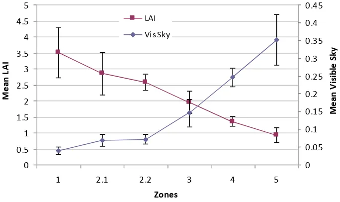
humidity data………...….41 Fig. 11 Box plots of visible sky (VisSky) proportion, leaf area index (LAI), total

below radiation (TotBe), direct below radiation (DirBe), diffuse below

radiation (DifBe) data by Johansson zone……….…43 Fig. 12 Mean visible sky and LAI for Johansson zones and above the canopy………...42 Fig. 13 Means in Johansson zones for total (TotBe), direct (DirBe), diffuse below

(10)

Fig. 14 A) Mean direct and diffuse fractions of radiation below the Weinmannia sp. crown as proportion of total above canopy radiation; B) variation in

ratio of direct to diffuse below crown radiation among zones………...….45 Fig. 15 Hemispherical images showing a typical sky proportion for each zone……….…….46 Fig. 16. Hourly mean temperature and relative humidity in Johansson zones and

above the crown, over the study period………...51 Fig. 17 Means of interquartile ranges for hourly relative humidity and temperature

in Johansson zones and above the canopy………...52 Fig. 18 Proportion of species confined to each zone and the proportion that zone

exclusive species contributed to the total number of bryophytes found

on the Weinmannia host (inset marker)……….…..61 Fig. 19 Hepatic and moss species and the ratio of hepatics to mosses (right) in

Johansson zones………..62 Fig. 20 The proportion of obligate mosses (light grey) and hepatics (dark grey) in

each zone……….63 Fig. 21 The south-western, more exposed side of the lower trunk. The white line

crossing the image is part of a grid delimiting subsections of a 1 ha

study plot used in complementary studies………...…..63 Fig. 22 Site 2.9. Thick species rich mats were typical along the sheltered side of

the trunk……….…….64 Fig. 23. Site 2.10, at the same height but opposite side of the trunk to the above

pictured site 2.9………...….64 Fig. 24 The high-rise of bryophytes - base of the eastern leader. Sixty four species

were found in zone 3 and a mean of 22.2 species were recovered from

0.03 m2_{samples………...………..65}

Fig. 25 The Weinmannia had an open, twiggy crown. Looking up the exposed side

of the trunk………..…….66 Fig. 26 Frullania riojaneirensis doing battle with fruticose lichens for supremacy of

the twig kingdom……….….66 Fig. 27 Species accumulation curve of the observed species (Sobs) on the Weinmannia

host and predictions of species richness by some of the popular estimators…..….67 Fig. 28 Fisher’s alpha and Simpson index for increasing number of epiphytic

(11)

Fig. 29 Rank-abundance plot for the bryophyte community on the Weinmannia sp. and a cumulative frequency-abundance class plot (Gray, 1981)

demonstrating the normal distribution of the collected species abundance

data………..….69 Fig. 30 Above - Classification of sample sites by similarity in species composition

(Bray-Curtis, group average linking, chaining = 12.8%); Below – Classification of zones by similarity of species frequency in zones

(Bray-Curtis, furthest neighbour linking, chaining = 0%)………...…73 Fig. 31 Classification dendrogram of a reduced species database (Bray-Curtis,

group average linking, chaining = 3.41%)……….….74 Fig. 32 NMS plot of species based on occurrence across similar samples of

epiphytic bryophytes on a Weinmannia sp. host………..…75 Fig. 33 The high light specialist Colura tenuiconis, ventral view……… …………...…….……76 Fig. 34 The decorative Lophocolea muricata with perianth……….…………...……….78 Fig. 35 Graphical representation of the variation in environmental variables among

sites as generated by PCA……….…95 Fig. 36 Graphical representation of the relationship between species composition and

environmental variables across sample sites, as interpreted by NMS ordination, with a joint plot overlay of variable vectors………...….96 Fig. 37 NMS ordination plots representing species composition and environmental

data collected on a Weinmannia sp. host in lower montane rainforest, Peru

(stress = 15.5)………...…97 Fig. 38 The number of hepatics and mosses found on 3 tree hosts. Sampling was stratified

by Johansson (1974) zones. The hepatic to moss ratio in each zone is indicated on the right……….……107 Fig. 39 Contribution of obligate species to the overall zone (Johansson, 1974) moss

and hepatic species richness. Species presence was sampled with different methodologies on three tree hosts at 2400 m in lower montane

rainforest, Peru………..………..108 Fig. 40 Crown limited (zones 3-5), trunk limited (zones 1-2) and generalist species

(12)

List of tables

Table 1. Subsample study tree details, including location of zone samples……….26 Table 2. Proportion of a known sample species population revealed by 1 to 6

subsamples………..…..28 Table 3. Proportion of a known zone species population revealed by 1 to 12

subsamples (pooled data from Alchornea sp. and Croton sp. individuals)……….…28 Table 4. Associations between radiation related variables. All correlations (as

Pearson’s r) were significant at P < 0.001………..……47 Table 5. Similarity between zone relative humidity (RH) medians, as identified

by a Bonferroni adjusted Mann-Whitney test. RH medians in zones with

the same letter was found to be statistically similar………47 Table 6. Statistical similarity of zone medians amongst the radiation associated

variables revealed by Mann-Whitney pairwise comparisons………...….48 Table 7. Means for temperature, relative humidity, photosynthetically active

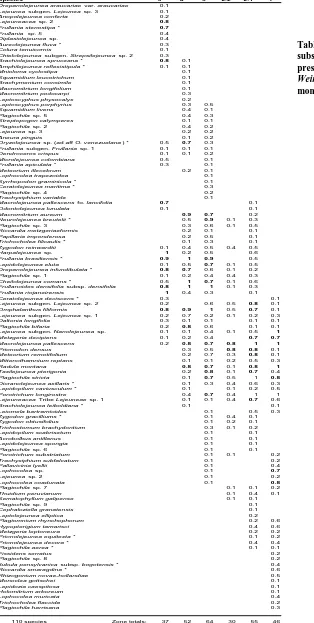
radiation and precipitation for October and November (Catchpole, D. 2007, pers. comm.) and values for the same period in 2006………....….53 Table 9. Genera with highest number of species on the Weinmannia host……….….59 Table 8. The proportion of subsamples in which taxa were present in each zone of a

single Weinmannia sp. host, lower montane rainforest, Peru………....…60 Table 10. Slope of a linear regression of rank (x) on frequency of occurrence (abundance)

in zone samples (y)………...….…69 Table 11. Whittaker’s estimate for turnover within zones (βw in zone), all species between

zones (βw all), hepatics between zones (βw hep) and mosses between zones (βw moss)...70

Table 12. Estimate of similarity in species composition between pairs of zones by the

Jaccard and Sørensen indices………70 Table 13. Ranking of similarity between assemblages of mosses and hepatics in each

zone by the Jaccard index. (15 = most similar)………....…..71 Table 14. Jaccard and Sørensen estimates of similarity between upper and lower trunk

(13)

Table 17. The upper trunk community……….………78

Table 18. The lower trunk community………....……..79

Table 19. An overview of species capture by studies in various habitats………..……..80

Table 20. Correlation of environmental variables (Pearson’s r)……….……93

Table 21. Above - eigenvalues for the first 9 axes of the environmental data PCA……....….94

Table 22. Highest correlations of environmental variables to the first NMS axis………....…96

Table 23. Frequency in zone samples of six species with wide distribution on the Weinmannia sp.. …………...…………...……..……98

(14)

Chapter 1. Introduction

The “tropics” are not a plot of convenient forest in Costa Rica; they are an

enormous realm of patchiness, and any theoretical thinking based on

presumed general properties is bound to become an in-group exercise in

short-lived futility.

- Paulo E. Vanzolini

The Neotropics are home to nearly 4000 bryophyte species or one third of the world’s

population (Gradstein et al., 2001a). This disproportionate diversity, also recorded for

vascular species, is higher than found in tropical Africa or Australasia and may be a

consequence of the extremely broad range of habitats afforded by an altitudinal and

climatic gradient stretching from the humid lowland Amazonia to the glaciated peaks of

Huascaran (6768 m) and the dry Pacific slopes of the tropical Central Andes. Of the 595

bryophyte genera in 120 families, 80 moss and 50 hepatic genera are endemic to tropical

America, making it the world centre of generic endemism (Gradstein et al., 2001a).

The tropical Andes have long been recognized as the jewel in the biodiversity crown of

the Neotropics (Gentry, 1992b). The region boasts an estimated 800-900 hepatics

(liverworts and hornworts) and 1200-1400 moss species (Gradstein et al., 2001a). Most

diverse moss families include Dicranaceae (gen. 34/190 sp.), Daltoniaceae (9/200),

Pilotrichaceae (21/200), Grimmniaceae (8/50) and Pottiaceae (55/361), contribution of the

latter two becoming greater in the dryer areas of the south. Hepatics in the tropical

Andes are rich in Gondwana groups that reach their widest distribution in temperate

Southern Hemisphere and reoccur at high elevations in the tropics. Lejeuneaceae is by far

the most species rich hepatic family, with 70 genera and approximately 400 species. Other

diverse families are Lepidoziaceae (16/110), Plagiochilaceae (4/112) and Jubulaceae

(15)

Woody plant diversity decreases above 1500 m. However, bryophytes reach their peak

species richness in upper montane cloud forests at 2500-3000 m, where cooler

temperatures and high frequency of moisture bearing low cloud encourage luxuriant

growth of this ectohydric group of plants (Gentry, 1992b; Gradstein, 1995; Gradstein et

al., 2001a). Tropical montane cloud forests occur between 1500-3300 m and in the

Neotropics stretch over both the lower montane (1000/1400-2000/2500 m) and upper

montane (2000/2500-3000/4000 m) rainforest types (Bruijnzeel and Proctor, 1995b;

Gradstein et al., 2001a). Population pressure is pushing more colonists into the Andean

montane forests. Both lower montane and upper montane forests are being cleared for

timber, charcoal production and conversion to pasture and agriculture. In the north, 90%

of cloud forest has already been cleared (Doumenge et al., 1995), while in the Central

Andes, Young (1992a) identified the lower montane forest as historically at greatest risk

of conversion, although data about the more recent trends are not easily available.

Considering the area occupied by montane forest, they are being modified at a greater rate

than the lowland forest of Amazonia. This statistic is even more alarming in the light of

the greater species diversity in montane forests than in Amazonia. The Northern Andes is

estimated to support 40,000 species of flowering plants in an area 20 times smaller than

the Amazon basin, which supports an estimated 30,000 species (Henderson et al., 1991).

Besides their considerable contribution to the overall biodiversity of the region,

bryophytes also contribute to the hydrological and nutrient cycles of montane forests

(Veneklaas et al., 1990; Coxson and Nadkarni, 1995). Epiphyte branch cover in upper

montane cloud forests can exceed 80%, with bryophytes heavily contributing to this value.

Harvesting of horizontal precipitation by tropical montane cloud forests can contribute an

additional 5-20% to the annual rainfall (Bruijnzeel and Proctor, 1995b), with this function

particularly valuable during the dry season. Chang et al. (2002) have shown that

bryophytes are efficient captors of fog. Their experiment, carried out in montane cloud

forest in Taiwan, revealed that on average 0.63 g of water was deposited per gram of

bryophyte dry weight per hour, translating to 0.17 mmh-1 on a stand scale or 36% of the

(16)

much as 50% of wet deposited inorganic nitrogen (NO-3). This has important

consequences not just for the availability of this essential and very mobile nutrient in wet

montane forests, but like the intercepted horizontal precipitation contribution to stream

flow, impacts on ecological processes far removed from the stream headwaters (Burns,

2003; Luo et al., 2007). Despite these apparent ecological services, bryophytes remain

poorly studied in the Neotropics and particularly so in the Central Andes of Peru and

Bolivia (Gradstein et al., 2001a). There is a pressing need for bryophyte species

inventories to provide baseline diversity data to assist in conservation planning and to

provide a foundation for further investigations of species dynamics and function.

Most of the species in rainforests are epiphytes; only 20% of those are shade epiphytes

restricted to the low light and very humid environment of the understorey in undisturbed

rainforests (Gradstein et al., 2001a). Variation in species abundance throughout a tree

crown reflects the individual taxa tolerance limits of environmental parameters, as well as

colonization and turnover dynamics (Proctor, 1981; Van Leerdam et al., 1990). A

gradient of temperature, relative humidity and availability of photosynthetically active

radiation exists from the trunk base to the outer crown and crown centre to outer crown,

creating a mosaic of microclimates. Many epiphyte studies have adopted the Johansson

zonation system to divide a host into microclimatically distinct areas (Johansson, 1974;

Van Leerdam et al., 1990; Kelly et al., 2004). Although bryophyte species are quite

sensitive to climate and habitat characteristics, the geographic distribution of individual

species in the Neotropics is much broader than that of vascular plants (Gradstein et al.,

2001a). Studies in tropical rainforests have shown that sampling of 3-5 trees may reveal

up to 80% of the local bryoflora (Wolf, 1993a; Gradstein et al., 1996; Gradstein et al.,

2003b).

1.1 History

Exploration of Andean bryophyte diversity begun a little over 200 years ago. The earliest

collections were those by José Celestino Mutis in Colombia (1783-1808) as subjects of illustrations in the “Flora de la Real Expedición Botanica del Nuevo Reino de Granada”,

(17)

Madrid Botanical Garden, is of greater historical than scientific significance, but has

resulted in some of the earliest illustrations of Andean bryophyte flora (Churchill and

Linares, 1995).

The earliest collections with a scientific interest were made by Alexander von Humboldt

and A. Bondand who collected a few moss and hepatic samples near Ibague during their

expedition to Colombia in 1801 grad. There was nearly a 40 year gap before J. Goudout

(1844-1845) among others continued the exploration of the new world. Perhaps the most

important collections of the 19th century were those of A. Lindig (1859-1865) and J. Weir

(1863-1864) in Colombia, W. Jameson in Ecuador, A. Moritz and W. Fender in Venezuela

and R. Spruce who collected in the latter half of the century in Colombia, Ecuador and

northern Peru (Hampe, 1847; Churchill and Linares, 1995). His Hepticae et Andinae is

still considered a landmark along the path to the modern understanding of Andean

bryophyte flora (Spruce, 1884-1885; Gradstein, 1995).

The 20th century saw more frequent participation by local botanists like H. Garcia

(1934-74) and L. Uribe U. (1939-72), assisted by north Americans W. L. Steere (1942-45) and F.

R. Fosberg (Churchill and Linares, 1995). T. Herzog's expedition to Bolivia in 1916 and

1920 greatly advanced the knowledge of the otherwise little investigated Bolivian

bryophytes (Churchill and Linares, 1995; Gradstein, 1995). Descriptive and taxonomy

focused studies continues into the latter half of the 20th century with important works in

the Colombian Andes by H. Bischler (1964), R. M. Schuster in Venezuala (1978) and E.

and P. Hedgewald in peru (1977), among others. More recent studies conducted under the

umbrella of the Dutch-Colombian Ecoandes project (Gradstein, 1982; van Der Hammen

and Ruiz, 1984) and the BRYOTROP project in northern Peru (Frey, 1987; Kürschner

and Parolly, 1998) among others (Gradstein et al., 1990) adopted a broader focus that

included bryophyte ecology and phytosociology. Wolf's description of communities along

an elevation gradient spanning between 1000 m and 4133 m in the Santa Rosa de Cabal

range, Colombia (Wolf, 1993b; Wolf, 1993c), the work of Gradstein and associates in

(18)

transect of H. Kürschner and G. Parolly in northern Peru (280-3300 m) (1998) provide an

invaluable insight into the ecology of bryophytes in montane habitats.

1.2 Objectives

This thesis presents the findings of a crown to ground epiphytic bryophyte survey

conducted in a lower montane cloud forest on the eastern foothills of the Andes (Peruvian

Yungas), Pasco, Parque Nacional Yanachaga-Chemillén. This is the first study of its kind

in the Selva Central of Peru and one of few for Peru.

The objectives were to:

i) determine the size of a representative subsample for the forest type in

the study area,

ii) characterise the microclimatic variation throughout a single tree host in

lower montane rainforest,

iii) determine the diversity of epiphytic bryophytes on a single tree host in

lower montane rainforest,

iv) identify environmental variables that may have the greatest influence

on the distribution of individual species within a host crown in lower

montane rainforest.

1.3 Structure of the thesis

A brief review of methodology applied in epiphytic bryophyte studies and results of a pilot

study to determine the minimum subsample size are presented in chapter 2.

A description of the microclimatic variation throughout the tree host is provided in chapter

3.

The findings of a single tree epiphytic bryophyte survey are presented in chapter 4. This

chapter also includes the description of four epiphytic bryophyte communities identified

(19)

Results of ordination species and environmental data are presented in chapter 5. A

discussion about the ability of some of the examined variables to explain the observed

species distribution is also included.

The concluding chapter 6, provides a summary of the major findings of the present study,

suggests a sampling methodology for future epiphytic biodiversity studies in the lowland

rainforest of the Yanachaga-Chemillén Range and identifies themes for potential future

studies of bryophyte ecology Peru.

(20)

Chapter 2. Methods

2.1 Study area

The study was conducted in lower montane rain forest on the isolated

Yanachaga-Chemillén Range forming the eastern flank of the Peruvian Andes, Department of Pasco,

central Peru. The approximately north-east extending range is included in the

Yanachaga-Chemillén National Park (120,000 ha) and includes lowland rainforest along its eastern

border, grading into lower montane and upper montane rain forest. The altitudinal range of

the park is 400-3800m, with the tallest peaks near the western extremity of the park.

The area is under the influence of a moist easterly air stream originating as the Atlantic

trade winds in the east. The moist air, recharged by the passage over the central Amazon

basin, is redirected to the south by the Andes (Killeen et al., 2007). Orographic lifting

results in locally high precipitation on the eastern flanks of the Andes, including the

Yanachaga-Chemillén Range. The area experiences a pronounced dry season between

April and September (Fig. 2). Low cloud is common throughout the year. Hillsides are

steep (20-60˚) and landslides common, even in undisturbed forest.

The study site was located at 2400 m a.s.l. on the leeward slope of the range, near its

western extremity (10.32 S, 75.21 W). Mean annual precipitation is 2703 mm and mean

annual temperature is 13.7˚C 1. Expected annual levels of photosynthetically active

radiation and mean annual relative humidity are 23.28 kmol.m-2.yr-1 and 93.4%.

The emergent stratum (to 38 m) of the surrounding forest is dominated by Cedrela

montana. Co-dominant species form a broken canopy of 20-25 m and include Nectaria

reticulate, Ficus gigantosyce, Guarea kunthiana, Ruage pubescens, Croton and

Weinmannia species. The understorey includes small trees and shrubs in the families

Ericaceae, Gesneriaceae, Melastomataceae, Piperaceae and Rubiaceae. Tree ferns in the

1_{Climate data for the site was recorded since 2003 and is provided here courtesy of Damien Catchpole, UTAS. Expected}

PAR is the above canopy value calculated from a hemispherical image.

(21)

Chapter 2. Methods

genera Alsophila, Cyathea and Dicksonia are common. Most tree and shrub stems are

covered with bryophytes. Vascular epiphytes are numerically dominated by Orchidaceae

(Catchpole, 2004). Species in families Araceae, Bromeliaceae, Dryopteridaceae also

[image:21.612.152.541.186.485.2]

abound in the crowns (Fig. 1).

Fig. 1 Lower montane rainforest near the study “El Cedro” site at 2400 m.

The site has been selectively logged for Cedrela montana and Podocarpus oleifoliusup

to some 20 years ago. However, species richness of the community remains quite high.

A complementary study of a 1 ha plot including the site of the current study found 134

woody species among 516 individuals with diameters greater than 0.1m (Requena Rojas,

2007); 195 species of vascular epiphytes were found in a nearby emergent Ficus sp.

(22)

Chapter 2. Methods

[image:22.612.175.508.85.560.2] [image:22.612.177.505.94.317.2]

Fig. 2 Mean monthly relative humidity, photosynthetically active radiation (PAR) , precipitation

and temperature at “El Cedro”, Yanachaga-Chemillén National Park, Peru (Catchpole et al.,

(23)

Chapter 2. Methods

2.2 Methodology review

It is difficult to compare the findings of most species diversity studies, not just because of

the variation in sampling technique, but also due to the myriad of methodologies employed to obtain a “representative” sample of the true populations. The techniques vary

greatly in their emphasis on quantitative accuracy and species capture, potentially leading

to contradictory findings about the characteristics of a community, dependent on the

technique and method used (Newmaster et al., 2005).

Relevé sampling intensively inspects large areas. Its emphasis is on gathering species

presence information (Braun-Blanquet, 1932; Newmaster et al., 2005). Floristic habitat

sampling adopts a slightly more rigorous method, more attuned to the accepted close

relationship between bryophyte species and microhabitat characteristics (Bouchard et al.,

1978; Proctor, 1981), despite their overall broad geographic ranges (Gradstein et al.,

2001a). Some studies have used a list of microhabitats (rocks, logs, cliff crevice, stream

side etc.) present within a mesohabitat (type of forest or landscape unit) to further

formalise the sampling process (Vitt and Belland, 1997; Newmaster et al., 2005). A

survey may be considered adequate when no singleton species remain. Plot sampling

includes a vast array of methodologies, from pin frame samples to area and time limited

sampling. Tokeshi (1993) advises that at least 10 samples should be collected to facilitate

sound statistical analysis. Different plot shapes have been used: square, rectangular, strip

and line plots, each shown to differently capture within landscape habitat heterogeneity

(McCune and Lesica, 1992; Gradstein et al., 1996; Eldridge et al., 2003). The opportunity

to mix and match these approaches is endless.

There is a positive relationship between the overall species richness and sample size

(Magurran, 2004). Large single areas have been shown to better capture species richness

than plot samples of an equivalent area (McCune, 1988; McCune and Lesica, 1992;

Archaux et al., 2007). However, the more extensive methodologies are criticised for their

poor quantitative accuracy (species abundance) (Archaux et al., 2007; McCune and

(24)

Chapter 2. Methods

communities. However, in there lays a paradox as many of the species richness

descriptors rely on information about the rare species that may be overlooked by plot

sampling methodologies (Newmaster and Bell, 2002).2 In short, the negative relationship

between species capture and quantitative accuracy seems to grade from large single

samples being best at revealing species richness, to intermediate performance of elongate

plot samples, with small sample areas providing most reliable abundance measures

(McCune and Lesica, 1992; Newmaster et al., 2005; Archaux et al., 2007). One needs to

be careful when interpreting findings of other studies, but also be clear about the purpose

when designing a study and be aware of the shortcomings of the adopted sampling

methodology.

Difficulties in comparing the findings from multiple studies have long been recognised. A

group of prominent ecologist has been working on a standardised methodology for

investigation of various components of epiphytic species diversity in tropical

environments (Gradstein et al., 1996). The latest “protocol for rapid and representative

sampling of vascular and non-vascular epiphyte diversity of tropical rain forests” has been

presented by Gradstein et al. (2003b). Based on numerous studies, they suggest that the

minimum sample size for vascular epiphytes does not need to be large. Sampling of just

eight trees and surrounding 20 x 20 m plots revealed 80% of the estimated total vascular

species richness for 1 ha of a Bolivian montane forest (Krömer, 2003). The minimum

sample size for non-vascular epiphytes is even smaller. Sampling of 3-5 trees identified

75-80% of total bryophyte diversity of a tropical forest (Acebey et al., 2003). For

epiphytic bryophyte diversity studies, Gradstein et al. (2003) suggest sampling just 5 trees

and woody vegetation within a 20 x 20 m plot around each tree. Sampling of trees should

be conducted in five Johansson (1974) zones using 5 subsamples in each zone3. The

2_{Information on the infrequent species is necessary to reveal the mode of the parametric lognormal species abundance}

distribution, frequently hidden by the “veil line” in incomplete surveys. Magurran AE (2004) 'Measuring biological diversity.' (Blackwell) . Popular non-parametric estimators of Anne Chao, like the Chao1, Chao2, ACE and ICE all rely on rare species data to derive their estimates of species richness. Chao A (1984) Non-parametric estimation of the number of classes in a population. Scandinavian Journal of Statistics 11, 265-270.; Chao A, Hwang WH, Chen YC, Kuo CY (2000) Estimating the number of shared species in two communities. Stat. Sinica10, 227-246.

(25)

Chapter 2. Methods

subsample size in zones 1-3 should be randomly positioned by cardinal direction and

measure 300 x 200 mm. Plots on branches in zones 4-5 should be 600 mm long, 3 located

on the upper and two on the lower branch surface, with total area dependent on branch

size.

The lack of basic species presence data for this region and Peru in general, and very

limited resources for this project force the adoption of a species capture focus. Similar to

other groups of plants, bryophyte species richness varies between different landscape units

or forest types. In the Neotropics, bryophyte diversity increases with elevation and peaks

in the cloud forests of the upper montane belt at 2500-3000 m before dropping again in

sub-alpine formations (Wolf, 1995; Gradstein et al., 2001a). Is it likely that one sampling

method can adequately capture species diversity across this gradient of species richness

and the mosaic of habitats? From the introduction above, it is clear that more extensive

studies yield more complete species lists and some type of stratification by microhabitat of

the sampling effort is desirable to most efficiently use limited resources.

But, how large does a subsample need to be to capture at least 75% of the epiphytic

bryophyte species richness in each section of a tree, in lower montane rainforest on the

Yanachaga-Chemillén Range, Peru?

2.3 Minimum subsample study

2.3.1 Methods

- Two mature canopy codominant trees (Table 1) were selected on the following criteria:

i) apparent richness in epiphytic bryophytes,

ii) contrasting bark type and crown structure,

(26)

Chapter 2. Methods

Table 1. Subsample study tree details, including location of zone samples.

Zone height / diameter (m)

Family Species Hgt (m)

Dia.

(m)* Notes 1 2 3 4 5

Euphorbiaceae Alchornea sp.

25.5 0.42 _{Complex, dense crown of strong} upright young leaders amongst older, previously broken ones. Young bark smooth, older shallowly fissured with prominent lenticels.

1.5 / 0.42 10/ 0.37 19.5/ 0.23 22/ 0.07 24.5/ 0.03 Euphorbiaceae Croton sp.

29.7 0.51 Open decurrent crown, home to a pair of nightjars. Bark smooth throughout. Sap, locally known as "sangre de grado" (blood of the dragon) has medicinal uses as antiseptic on wounds, for fighting stomach infections and ulcers.

1.5 / 0.51 9/ 0.25 20.7/ 0.19 25.5/ 0.09 28.2/ 0.03

* - Trunk diameter measured at 1.3m (DBH)

- A contiguous grid of 6 subsamples of 100 x 100 mm was established in each zone in the two trees. In zones 1-3, the collective sample size was 300 x 200 mm and

600 mm of branch length in zones 4-5. Where possible, the sampling grid was

placed across the trunk or branches in zone 3 to reduce redundancy of microsites

with similar light characteristics. Cardinal aspect of the collections was not

considered. Collections were made on the 19th and 20th of May, 2006.

- The crown was accessed with single rope and arborist techniques (Perry, 1978; Dial, 1994).

- Morphospecies within each subsample were identified using dissecting and compound microscopes.

- The morphospecies data for each sample and across zones in the two trees was examined using sample based rarefaction curves (species accumulation curves)

generated in EstimateS programme (Colwell, 2005). The curves were calculated

(27)

Chapter 2. Methods

- The relationship between the number of morphospecies recorded in entire and reduced samples was examined with the aid of MINITAB v.14 (14.12.0)

programme (Minitab Inc., 2000)

2.3.2 Results

A total of 99 morphospecies (72 hepatics and 27 moss sp.) were found on the Alchornea

sp. and Croton sp., 81 and 65 morphospecies respectively. The Alchornea sp. shared the

same number of morphospecies in zone 4 with the Croton sp., but had fewer in zone 2

(Fig. 3). One subsample from zone 3 of the Alchorea sp. included 35 morphospecies,

while average number across all subsamples was 15.6.

0 5 10 15 20 25 30 35 40 45 50

1 2 3 4 5

Zone

Sp

ec

ie

s

ri

ch

n

es

s

Alchornea sp.

[image:27.612.211.467.331.551.2]

Croton sp.

Fig. 3 Zone species richness in the Alchornea sp. and Croton sp. hosts.

Inspection of the species accumulation curves generated for all samples revealed a

common trend. 75-85.5% of the known species richness included in each sample was

collected in just 3 subsamples (Table 2). Pooled subsamples and morphospecies across

(28)

Chapter 2. Methods

Table 2. Proportion of a known sample species population revealed by 1 to 6 subsamples.

1.1 1.2 2.1 2.2 3.1 3.2 4.1 4.2 5.1 5.2

1 58.70 52.23 50.00 49.29 54.26 50.94 54.69 48.44 51.00 46.43

2 73.76 70.43 68.42 67.50 72.77 69.34 74.78 69.16 68.65 62.86

3 83.59 81.33 79.74 79.17 83.19 80.43 85.47 81.25 79.41 75.00

4 90.72 89.33 88.05 87.79 90.36 88.37 91.88 88.97 87.47 84.79

5 96.02 95.57 94.74 94.46 95.74 94.77 96.34 94.78 94.12 92.86

6 100 100 100 100 100 100 100 100 100 100

50 60 70 80 90 100

1 2 3 4 5 6

Subsamples P ro rt io n o f sp ec ie s 30 40 50 60 70 80 90 100

1 2 3 4 5 6 7 8 9 10 11 12

Subsamples

Fig. 4 A) Alchornea sp. zone 1 species rarefaction as proportion of species from a known

population; B) zone 4 species rarefaction curve (pooled data from Alchornea sp. and Croton

sp. individuals).

Table 3. Proportion of a known zone species population revealed by 1 to 12 subsamples (pooled

data from Alchornea sp. and Croton sp. individuals).

1 2 3 4 5

1 37.42 31.38 36.73 37.50 32.96

2 55.07 48.76 55.97 55.43 47.48

3 66.25 60.35 67.80 65.89 57.26

4 73.96 68.85 75.73 72.82 64.70

5 79.70 75.47 81.41 77.95 70.87

6 84.26 80.79 85.71 82.09 76.26

7 88.02 85.26 89.12 85.64 81.13

8 91.18 89.09 91.93 88.84 85.52

9 93.89 92.38 94.32 91.82 89.57

10 96.23 95.26 96.42 94.64 93.26

11 98.25 97.79 98.31 97.34 96.74

12 100 100 100 100 100

Zone

[image:28.612.138.542.107.383.2] [image:28.612.201.484.531.713.2]

(29)

Chapter 2. Methods

The ranking of total number of observed species was strongly negatively correlated with

the proportion of species captured with 3 subsamples (Fig. 5)

74.00 76.00 78.00 80.00 82.00 84.00 86.00 88.00

0 1 2 3 4 5 6

Rank observed

Pr

o

p

o

rt

io

n

o

b

se

rv

e

d

Fig. 5 Plot of rank of observed species in 5 Johansson zones (sample area of 0.06 m2) and

proportion of observed species captured in 0.03 m2 in each zone.

2.3.3 Discussion

The effort required to process the samples from this small pilot study was substantial. On

average, each subsample took one day to separate into morphospecies. The time required

to complete this study certainly reflects the inexperience of the author with tropical taxa,

but also highlights the species richness of the local bryophyte community. An average of

15.6 morphospecies was identified in each square decimetre and 35 were present in one

subsample from zone 3 of the Alchorea sp.

The samples consisted of interwoven mats of predominantly weft and mat growth-forms

in zones 1-4, giving way to tightly adpressed mats and individual wefts in zone 5. A large

proportion of the species are less than 1 mm across the leafy stems. The advice of

Gradstein et al. (2003b) to separate individual species and attempt their identification

under field conditions does not seem practical. Many morphologically similar hepatic

taxa, particularly among the Lejeuneaceae, and moss species can only be separated

[image:29.612.194.494.146.317.2]

(30)

Chapter 2. Methods

following close examination of their anatomy and cytology, to say nothing of the

morphologic plasticity within taxa.

The EstimateS programme used to produce the rarefaction curves and others, like

PC-ORD, do not consider the spatial arrangement of samples. Samples are assumed to be

non-contiguous (Scheiner, 2003). The worst case of subsample distribution under the

present grid system (3 x 2 subsamples) would be two adjacent subsamples and one

separated by 100 mm, a feature that needs to be considered when designing a larger study.

The ranking of the proportion of species captured by three subsamples within each zone

may reflect the overall zone species density (Table 3). The strong relationship between

rate of capture and overall species richness supports this hypothesis and justifies the doubt

expressed above about the efficiency of a single sampling method to adequately represent

the varying levels of species richness across different forest types (Fig. 5). Lennon et al.

(2001) found that local richness gradients had a large impact on beat diversity estimates

and others observed that species turn over is negatively related to species richness of an

area (Magurran, 2004). The method suggested by Gradstein et al. (2003) is likely to

underestimate the specie richness of less diverse assemblages, exaggerating the contrast

between those and species rich areas.

Gradstein (1995) used the number of hepatic epiphytes found on four trees to compare

hepatic richness in different tropical forest types. He found that the average number of

species in lower montane forest was 46 and in upper montane forest 86. This pilot study

conducted in the upper reaches of the lower montane belt, despite its very small sample

size, found 72 hepatics on just two trees. Could the bryophyte diversity of the forest on

the Yanachaga-Chemillén Range be greater than average?

2.3.4. Conclusion

The effort required to sample and process epiphytic bryophyte samples is montane

(31)

Chapter 2. Methods

unnecessarily large in lower montane cloud forest at 2400 m. on the Yanachaga-Chemillén

Range. Samples of half that size (0.03 m2) can capture 75% of the microsite species

richness. Smaller, but more numerous subsamples strategically placed across niche rich

habitats are likely to be more efficient and produce more accurate species richness

estimates than few large randomly placed samples. This is a contradictory finding to the

general belief that large samples are better at species capture than many randomly placed

small quadrats (McCune and Lesica, 1992; Archaux et al., 2007). The approach suggested

here is not dissimilar to the modified floristic habitat sampling stratified by microhabitat as

applied by Newmaster et al. (2004).

2.4 Single tree study design and methods

2.4.1 The host

A mature canopy co-dominant Weinmannia sp. was chosen as the subject of the single tree

bryophyte epiphyte survey (species name was not determined, despite expert assistance).

Weinmannia L., (Cunoniaceae R.Br.) is a genus of approximately 150 species of trees and

shrubs distributed throughout the montane regions of the Neotropics. Forty-one species

have been recorded for Peru (Pennington et al., 2004).

The tree was chosen for its unremarkable stature, average volume of epiphytes and

importantly, an architecture that promised access to the outer reaches of the crown. The

Weinmannia, unaffectionately called Tree 3, became Mannie over the course of the study.

It was 25.5 m high and its single trunk DBH (at 1.3 m) was 0.7 m. The crown had a

diameter of 10-12 m.

The tree was growing on a narrow shelf of a 40˚ sloping hillside, a north-eastern

escarpment of a narrow valley. The dense understorey occluded the trunk on the eastern,

slope side, but was thinner above 2 m. on the south-western side, leaving the trunk

exposed to the late afternoon sun. The shallowly buttressed lower trunk had a lean of approximately 4˚ into the valley, above a noisy stream some 30m below. Mid and upper

(32)

Chapter 2. Methods

The western side was very sparsely covered and had large, apparently bare areas coloured

by a patchwork of crustose lichens. It appeared obvious that the western side of the trunk

was exposed to the afternoon sun.

The fine, sparse crown was supported by two main leading branches spreading on along

an approximately north-south axis. Their bryophyte-mat covered bases had an

approximate diameter of 200 mm. Long and sinewy, the leaders rose some 11 m to the

twiggy pinnate leafed branch tips. Scaffold branches were few and distantly spaced. The

crown supported surprisingly few large bromeliads and the bryophyte mats were only

occasionally dotted with small orchid species. In the course of the study, a troop of

monkeys occasionally strolled through the nearby tree tops, humming birds were common,

but perhaps the most memorable was the visit by an Andean bear in a neighbouring

crown, and of course, the mosquitos!

2.4.2 Crown stratification and access

Stratification of the trunk and crown following Johansson (1974) is well established

among the canopy ecology researchers and will continue to be used in this study. It is

customary to divide the trunk into the base (generally the first two meters), the lower,

often more humid trunk section and the dryer upper trunk. As indicated above, the trunk

had a pronounced dry side – a common feature of trees in montane forest on steep slopes.

The division of the trunk and crown for the present study is illustrated in Figure 6.

(33)

Chapter 2. Methods

The crown was accessed with single rope and arborist techniques outlined by Perry

(1978), Dial and Toblin (1994) and Jepson (2000). The structure of the host permitted

access to within 1 m of most branch tips.

2.4.3 Floristic sampling and identification.

Epiphyte sampling, conducted in situ, was stratified by Johansson zone. Choice of

subsample location was guided by accessibility and the apparent microhabitat variation.

Ten subsamples were collected from each zone. Subsamples of 0.03 m2 (100 x 300 mm)

(34)

Chapter 2. Methods

of the local topography, cardinal direction was not considered during data collection.

Direct sunlight was blocked by the steep hillside to the north during a large portion of the

day.

Each subsample was placed in a paper bag and processes under both dissecting and

compound microscopes in the comfort of a laboratory. Species identification to genus

heavily relied on the excellent guide by Gradstein et al. (2001) for both hepatics (here

including both liverworts and hornworts) and mosses. A list of taxonomic literature is

provided in Appendix I. It was necessary to consult literature in Spanish, French, German

and English. The multilingual glossary for bryology, published by the Missouri Botanical

Garden proved invaluable (Magill, 1990). Identification of moss species was kindly

confirmed by Jasmin Alexandra Opisso Mejia, a bryologist at the Museo de la Historia

Natural, Lima. Unfortunately, no expert advice was available to confirm the hepatic

determinations.

A voucher collection was deposited at the Selva Central Herbarium (HOXA) of the

Missouri Botanical Garden.

2.4.4 Temperature and relative humidity

Both temperature and humidity data were collected

with LogTag HAXO-8 card loggers

(MicroDAQ.com). The loggers have a temperature resolution greater than 0.1˚C and 0.1% relative

humidity. The sensors were shielded with custom

built 6 plate radiation shields (Fig 7). The loggers

were suspended from custom built metal brackets

attached to branches and trunk. The sensor was

placed within 100 mm of the tree surface, in close

proximity to the epiphyte collection sites. Another

shielded LogTag logger was placed on a

(35)

Chapter 2. Methods

top of the tower and logger position was approximately 6 m above the forest canopy. The

loggers recorded temperature and relative humidity every 10 minutes.

Readings were taken between 15/10/06 and 29/11/06, corresponding to the transition

period between the dry and wet seasons in the Selva Central of Peru. In each zone, one

fixed and two roving loggers were used. The roving loggers were moved every 9 days to

a close proximity of one of 9 remaining epiphyte collection sites within each zone. A full

temperature and relative humidity data set for each sampling site was derived (using zone

1 as example):

i) regression of fixed logger in zone 1 (site 1) on mobile logger 1 (site 2) for

period 1,

ii) the regression model from above was applied to the complete study readings

for the fixed logger in zone 1 (x) to obtain expected complete study period

values for site 2 (y).

Relocation of the loggers took some hours. To allow for reaclimatisation of the shifted

loggers, a full day (day nine) was removed from the climate data.

2.4.5 PAR

Radiation data was obtained from a hemispherical image taken with a NIKON 4500

Coolpix digital camera (3.87 million pixels) and processed by the hemispherical image

analysis programme HemiView (Delta-T Devices Ltd., 2001).

The photos were taken with a FISHEYE 1 setting, sharpening function set to HIGH,

exposure set to -2.0 and using the 10 second timer to reduce jitter. Images were stored at

the highest available resolution. The camera was mounted on a custom built aluminium

staff fitted with perpendicular horizontal levels. The photographs were taken either early

in the morning or late in the afternoon to reduce reflections from foliage and bark. Despite

this, a number of images had to be adjusted to remove light coloured objects from below

the image horizon.4

(36)

Chapter 2. Methods

The solar model used in the calculation of incoming radiation by the HemiView

programme was calculated from real site data (Catchpole, 2004); 2900 μmol m-2s-1, yearly

average transmissivity is 0.39, diffuse proportion is 0.57

2.4.6 Statistical analyses

- Climatic and radiation data were examined and tested with various procedures within the MINITAB v.14 (14.12.0) programme (Minitab Inc., 2000).

o the Kruskal-Wallis test was used to examine the similarity between

medians,

o the Mann-Whitney pair comparison was used to identify similarity between

subsets of zone data.

- EstimateS 7.5.0 programme (Colwell, 2005) was employed to:

o generate species accumulation curves with 100 randomisations of the

sample data without replacement,

o generate species richness estimates and species richness indices,

o assess similarity in species composition between sites and generate

similarity indices.

- PC-ORD v. 4.27 programme (McCune and Mefford, 1999) was used to:

o generate classification dendrograms,

Normal classification was performed with species incidence data to reveal the

similarity between sites. Continuity in community composition was examined

with an inverse classification of species using sum incidence data. Species

with less than 2% frequency were excluded from the analysis (95 species

used). Both analyses were performed without any further transformation of the

data.

A number of distance measures and types of clustering were examined prior to

(37)

Chapter 2. Methods

o perform indicator species analysis,

The analysis employed the method of Dufrene and Legendre (1997).

o perform principal components analysis (PCA) on environmental data,

o perform non-metric multi-dimensional scaling (NMS) ordination,

The analyses performed 40 runs of real data, 50 runs of randomised data.

NMS ordination was performed on a reduced species set (95 species, species

with overall frequency of < 2% were excluded) and a reduced number of

(38)

Chapter 3. Microclimate

3.1 Background

Much has already been published about climatic variation in rainforests (Richards, 1952;

Walter, 1971). In contrast, few studies to date have investigated the microclimatic

gradients within tree crowns and fewer still have taken place in montane rainforests (Kira

and Yoda, 1989; Freiberg, 1997; Szarzynski and Anhuf, 2001; Cardelus and Chazdon,

2005; Catchpole et al., 2005). Sensitivity of bryophytes to variation of light, temperature,

moisture availability, substrate acidity among other factors is well accepted (Barkman,

1958; Proctor, 1981) and the distributional variation of species and growth-forms

throughout tree crowns has not gone unnoticed (Van Leerdam et al., 1990; Wolf, 1994).

Intra crown climatic variation could influence the physiology of both tree hosts and

epiphytes and may assist in forming hypotheses about the observed patterns of epiphyte

species distribution.

Temperature and relative humid generally follow opposing gradients from the ground to

the crown periphery (Kira and Yoda, 1989; Freiberg, 1997). In rainforests, coolest

temperatures generally occur near the ground. This coincides with the highest light

interception levels; on average, as little as 1% of the above canopy radiation reaches the

rainforest floor (Kira and Yoda, 1989). Highest temperatures and lowest humidity occur

in the outer crown, with corresponding low light interception.

The general pattern of diurnal fluctuation of temperature and relative humidity is much

more complex. As the crown heats up during the day, the warmer air in the crown is

decoupled from the cooler air in the understorey and turbulently mixes with the boundary

layer above (Szarzynski and Anhuf, 2001). The rise of temperature and drop in relative

humidity is much more pronounced in the outer crown than near ground level. At night,

radiative cooling at the top of tree crowns results in lower temperatures there than near the

ground, where loss of long-wave radiation is reduced by the overtopping canopy

(Freiberg, 1997; Szarzynski and Anhuf, 2001). There is little variation in humidity

(39)

Chapter 3. Microclimate

A contrasting diurnal pattern was found by Catchpole in his study conducted in a Ficus sp.

in close proximity to the present study site (Catchpole et al., 2005). There, the lowest

nightly temperatures occurred near the ground and above the crown, and maxima in the

crown. Day maxima were reached above the crown and minima in the mid-crown. He

attributes the observed climatic pattern to the characteristics of vascular epiphyte

distribution and crown structure.

Epiphytes in tree crowns may be influenced by microclimatic parameters, but they

themselves also modify the crown microclimate (Freiberg, 1997; Freiberg, 2001; Stuntz et

al., 2002). Temperature fluctuations immediately near branches were shown by Freiberg

(1997, 2001) to be moderated by the presence of epiphytes and crown humus. The effect

was strongest within 100 mm of the branch surface, with little difference beyond 0.75 m

away from the branch (Freiberg 2001). Elevated relative humidity and lower temperatures

associated with the moisture holding capacity of the epiphytic material and canopy humus

not only have the potential to reduce evapotranspiration at microsites near epiphyte

clumps, but also can significantly lower the moisture loss from their host (Stuntz et al.,

2002).

The objective of the present study was to describe the temperature, relative humidity and

radiation characteristics of a canopy co-dominant crown in lower montane rainforest,

during the transition period between dry and wet seasons in the Selva Central, Peru.

3.2 Results

Methods are presented in Chapter 2, section 2.4.

3.2.1 Temperature and relative humidity

Both temperature and relative humidity (RH) data collected from the crown were not

Epiphytic bryophytes and habitat microclimate variation in lower montane rainforest, Peru