Clustering of equine grass sickness cases in the United Kingdom:
a study considering the effect of position-dependent reporting on
the space–time
K
-function
N. P. F R E N C H1*, H. E. M
CC A R T H Y2, P. J. D I G G L E3A N D C. J. P R O U D M A N2
1Institute of Veterinary, Animal and Biomedical Sciences, Massey University, Palmerston North, New Zealand 2
Department of Veterinary Clinical Science and Animal Husbandry, University of Liverpool Faculty of Veterinary Science, Leahurst, Neston, Cheshire, UK
3Department of Mathematics and Statistics, Lancaster University, Lancaster, UK
(Accepted 4 October 2004)
S U M M A R Y
Equine grass sickness (EGS) is a largely fatal, pasture-associated dysautonomia. Although the aetiology of this disease is unknown, there is increasing evidence thatClostridium botulinumtype C plays an important role in this condition. The disease is widespread in the United Kingdom, with the highest incidence believed to occur in Scotland. EGS also shows strong seasonal variation (most cases are reported between April and July). Data from histologically confirmed cases of EGS from England and Wales in 1999 and 2000 were collected from UK veterinary diagnostic centres. The data did not represent a complete census of cases, and the proportion of all cases reported to the centres would have varied in space and, independently, in time. We consider the variable reporting of this condition and the appropriateness of the space–time K-function when exploring the spatial-temporal properties of a ‘ thinned ’ point process. We conclude that such position-dependent under-reporting of EGS does not invalidate the Monte Carlo test for space–time interaction, and find strong evidence for space–time clustering of EGS cases (P<0.001). This may be attributed to contagious or other spatially and temporally localized processes such as local climate and/or pasture management practices.
I N T R O D U C T I O N
Equine grass sickness (EGS) is a largely fatal, pasture-associated dysautonomia of unknown aetiology. The acute disease is characterized primarily by failure of normal alimentary function. The highest incidence of EGS is believed to occur in Scotland where the disease was first identified in 1907, although the disease also occurs throughout England and Wales (for a review see [1]). The temporal pattern of EGS has also been well described, with most cases occurring between April and July [2–4]. However, to date, little has been
done to explore the spatial patterns of EGS in England and Wales. In addition, no studies have considered the joint distribution of EGS cases in space and time.
The well-described spatial distribution might arise as a result of regional variation in the population at risk, reporting bias and other static variables associ-ated with the onset of disease (e.g. soil type, habitat and altitude). Likewise, the temporal pattern might be attributed to seasonal variation in risk factors such as temperature and pasture growth. However, we were interested in exploring the possibility that these spatial and temporal processes interact to provide space–time clustering. Such a situation can arise if there is a contagious element or spatially and tem-porally localized variation in other ‘ driving ’ variables.
* Author for correspondence : Professor N. P. French, Institute of Veterinary, Animal and Biomedical Sciences, Massey University, Palmerston North, New Zealand.
Estimating the extent of clustering might assist in the formulation of disease-prevention strategies in the face of a confirmed case.
There are many approaches to the exploration of space–time clustering in human and animal diseases. The Mantel test, Barton’s method, nearest-neighbour test and Knox’s test are techniques useful for in-vestigating space–time interaction. These and other methods are reviewed in refs [5–7]. Most of these tests concentrate solely on testing the null hypothesis of no space–time interaction and do not consider the scale or nature of space–time interaction. Diggle et al. [8] suggested an alternative approach, which provided a formal, edge-corrected test for space–time interaction and informal graphical methods for describing the nature and scale of space–time clustering. This method extends the use ofK-functions [9] (previously used to describe purely spatial point patterns) to spatial–temporal processes. The technique has been used to describe sporadic cases of human disease but has rarely been used in veterinary epidemiology [10, 11]. We use K-function analysis to examine space–time clustering of EGS in England and Wales and consider the effects of position-dependent under-reporting on the validity of the space–timeK-function.
M E T H O D S Data on EGS
Data from histologically confirmed cases of EGS in England and Wales were collected from UK veterin-ary diagnostic centres. Cases that were diagnosed from clinical signs only were excluded from the study due to the possibility of misdiagnosis. The date used was the date the horse first showed clinical signs or the date the horse was admitted to a veterinary hospital (if applicable). The former was used in preference. Because this is an acute-onset disease the difference between the two was likely to have been less than 2 days. The geographical location where the case occurred was identified as the nearest village or town to the premises where the horse originated. This would have been within 1–2 km of the premises (client confidentiality restricted the authors access to exact premises locations). Each location was converted into a four-figure Ordnance Survey grid reference using theOrdnance Survey Gazetteer of Great Britain(third edition). Information was collected on 133 histologi-cally confirmed cases of grass sickness in the years 1999 and 2000. Two datasets were used in the analysis. The
first comprised all reported cases including multiple cases from the same premises. The second was a slightly smaller (119 cases) database comprising only the first case to be reported on each of the premises during the study period. This smaller dataset was analysed to examine space–time clustering in the absence of very local (i.e. same premises) effects.
Space–time K-function analysis
The technique is fully described by Diggle et al. [8]. Briefly, the observed spatial–temporal point pattern is compared with a pattern that has the same temporal and the same spatial properties as the original data, but no space–time interaction. Like the Knox test this method does not require knowledge of the underlying population at risk. This involves the estimation of three component processes, i.e.K-functions :
K(s,t)=lx1
E [number of further events occurring within distancesand timetof an arbitrary event of the process],
K1(s)=l1x1 E [number of further events occurring within distance s of an arbitrary event of the process],
K2(t)=l2x1 E [number of further events occurring within timetof an arbitrary event of the process],
where E refers to the edge-corrected expected value [e.g. forK1(s) it is the mean number of events within distance s of an arbitrary event, adjusted for edge-effects],l is the expected number of events per unit space per unit time (intensity of the disease process), andl1andl2are the spatial and temporal intensities respectively.
The product of the spatial and temporal K -func-tions K1(s)K2(t) is the expectedK-function under the hypothesis of no space–time interaction and is used as a benchmark for comparison with the observed space–timeK-function :K(s,t).
In addition to providing an edge-corrected Monte Carlo test for space–time interaction (see [8] for full details), the method can be used to estimate and describe proportional and absolute increases in disease risk, attributable to space–time interaction, for a range of spatial and temporal separations. This is achieved by graphing three diagnostic functions. The edge-correction and the additional interpretation of the nature of space–time interaction are advantages of this method over the Knox test.
^ D
D(s,t)=KK^(s,t)xKK^
This function is proportional to the increased num-bers of cases within distance s and time t by com-parison with a process with the same spatial and temporal structures but no space–time interaction. It is analogous to the risk difference in epidemiology and is plotted againstsandt.
^ D
D0(s,t)=DD^(s,t)={KK^1(s)KK^2(t)}: (2)
This is proportional to the relative increase in cases within distancesand timetcompared with a process with the same spatial and temporal structures but no space–time interaction. It is analogous to the relative risk and is plotted againstsandt.
R(s,t)=DD^(s,t)=pffiffiffiffiffiffiffiffiffiffiffiffiffiffiffiffiffi{V(s,t)}, (3)
whereV(s,t) is the variance of Dˆ(s,t) [see [8] for the calculation ofV(s,t)]. When plotted againstK1(s)K2(t) this is analogous to a plot of the standardized residuals against fitted values. If the spatial and temporal processes were independent (i.e. there was no space–time interaction) then we would expect approximately 95 % of the values to lie between the values ¡2. A disadvantage of this plot is that the spatial and temporal scales are no longer explicit and the ‘ residuals ’ are highly interdependent. Rather than a ‘ cloud ’ of points, this lack of independence may produce obvious patterns (e.g. lines of points) within the plot. We suggest that for most applications, the functionDˆ0(s,t) will be of most interest.
Considering the effects of position-dependent thinning (systematic under-reporting)
The data used in this analysis were not a complete census of all cases in England and Wales. Furthermore, the proportion of all cases of EGS included in the analysis varied according to geographical location and may also have varied over time. This is termed ‘ position-dependent thinning ’ and arises from the variation in case reporting throughout the region studied (for example it is likely that proportionally more cases were ascertained in areas closer to the contributing diagnostic centres). This means that the spatial distribution of the cases used in this analysis does not represent the true underlying spatial distribution of EGS cases in England and Wales. Likewise there may be times of the year when proportionally fewer cases are reported. Although tests for purely spatial or purely temporal clustering would be affected by position-dependent thinning or
temporal-dependent thinning respectively, we show that the Monte Carlo test for space–time interaction used in this analysis is not invalidated by such thinning, provided the spatial and temporal thinning operate independently.
For a more formal consideration of the effect of position-dependent thinning on the test of no space–time interaction we consider a spatio-temporal dataset (xi,ti) :i=1, …,ngenerated by a process with no space–time interaction. Hence the complete set of spatial locations,X=(x1, …,xn) is independent of the complete set of temporal locations,T=(t1, …,tn). A spatio-temporal thinning is defined by a function p(x,t) denoting the probability that a point survives in the thinned process, given that it is at space–time location (x,t). If spatial and temporal thinnings operate independently, thenp(x,t)=p1(x)p2(t). If we assume that spatial and temporal thinnings are inde-pendent we can imagine the thinning to take place in two stages : the first according to the spatial thinning functionp1(x) ; the second thinned from the survivors of the first stage according to the temporal thinning functionp2(t). If we call the temporal locations which survive the first stage of thinningT*, and the surviv-ing spatial locations X*, then under the stated assumptions, T* consists of a random sample from the original set T. Since T is independent of X, it follows that T* is independent of any subset of X chosen without reference to T, and in particular is independent ofX*. HenceX* andT* are independent and a test of no space–time interaction in the dataX*, T* is a valid test of no space–time in the original data X, T. If we repeat the argument, applying a second thinning toX*,T* according to the temporal thinning functionp2(t), and reverse the roles of the spatial and temporal locations, we produce thinned data X**, T**. A test of no space–time interaction inX**,T** is also a valid test of no space–time interaction inX*, T* and hence in the original dataX,T.
All analyses were performed using the SPLANCS library [13] in S-PLUS (Insightful Corporation, Seattle, WA, USA).
R E S U L T S
Temporal and spatial patterns of EGS
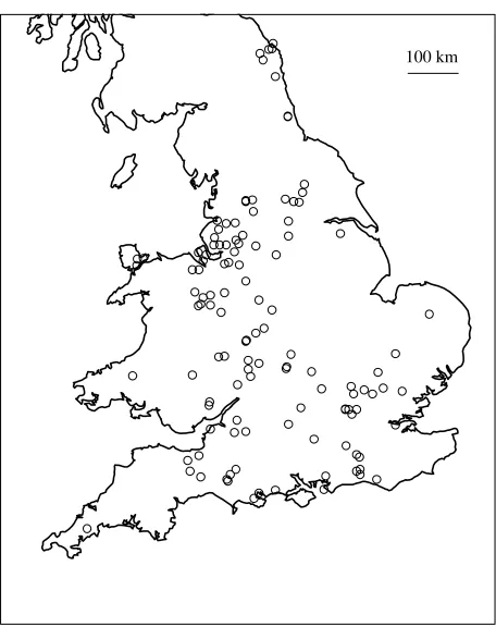
Figure 1 shows a peak in May in the temporal pattern of the 133 EGS cases used in this study. Figure 2 shows the spatial distribution of the 133 histologically confirmed cases of EGS used in this study. The apparent spatial clustering of EGS cases in several parts of England and Wales is potentially misleading. This is most likely due to uneven, clustered reporting of cases, particularly around the major contributing diagnostic centres. Hence purely spatial thinningp(x) is a plausible feature of the problem.
Space–time K-function analysis
When all cases were considered together there was strong evidence of space–time clustering of EGS cases. The Monte Carlo test for space–time interac-tion computed aPvalue of<0.001 providing formal evidence for space–time interaction. The residual plot (Fig. 3) ; referring to spatial separations up to 30 km (in 5-km increments) and temporal separations up to 90 days (in 4-day increments), revealed that almost all of the residuals were >2. This indicated space–time interaction over wide spatial and temporal separ-ations, but particularly for lower values of K1(s)K2(t) corresponding to shorter spatial and temporal dis-tances. This is confirmed by the Dˆ(s,t) plot which showed a sharp rise over the first 10 km and 20 days
(not shown) and demonstrated further in theDˆ0(s,t) plot (Fig. 4) which showed the greatest proportional increase within these distances. High values on the z axis of theDˆ0(s,t) plot indicates that there are many more outbreaks within the given spatial and temporal separation than would be expected if there were no space–time clustering.
When multiple cases were excluded from the analysis this left 119 EGS outbreaks (incident cases). The R(s,t) and Dˆ0(s,t) plots of the 119 EGS outbreaks (Figs 3 and 4) also showed that a large proportion of incident cases within 10 km and 20 days of each other could be attributed to space–time clustering. Thus the exclusion of multiple cases still revealed significant evidence of clustering. The Monte Carlo test for space–time interaction computed a Pvalue of 0.016.
D I S C U S S I O N
By providing both an edge-corrected test for space– time interaction and an estimate of the nature and extent of the process, theK-function has advantages over the Knox test. Furthermore, this method comp-lements the many other approaches to the analysis Jan. Feb. Mar. Apr. May June July Aug. Sept. Oct. Nov. Dec.
0 5 10 15 20 25
[image:4.595.320.548.63.351.2]No. of cases of equine grass sickness
Fig. 1.Seasonal distribution of 133 histologically confirmed cases of equine grass sickness during 1999 (%) and 2000 (&) in England and Wales.
100 km
[image:4.595.77.300.65.227.2]of data with both a spatial and temporal dimension. For example, the space–time scan statistic [14] is use-ful for identifying the location of individual clusters or ‘ galaxies ’ of disease in space–time cylinders. In contrast, K-function analysis helps to describe the more general properties of a space–time process.
In this study it was highly likely that the proportion of cases reported varied across and within regions due to variable degrees of under-reporting by veterinary surgeons and pathologists. Temporal variation in the degree of under-reporting could also occur if, for example, a diagnosis was less likely to be made outside the high-risk months of April, May and June. K-function analysis is not invalidated by random under-reporting or ‘ thinning ’. Furthermore, the test for space–time interaction is not invalidated by position-dependent under-reporting, provided the spatial and temporal thinning were independent. Therefore, unless there was an interaction between spatial and temporal variation in reporting (e.g. a veterinary surgeon reported all cases within a small area over a short time period and only a fraction of other cases encountered) under-reporting would not have invalidated the test for space–time clustering.
This study provided strong evidence for space–time clustering of grass sickness cases in the United Kingdom. Space–time clustering was evident both
when individual EGS cases and individual outbreaks of EGS were investigated. The presence of a space– time interaction on such a local scale is consistent with either an infectious aetiology, and/or risk factors that localize both spatiallyandtemporally.
The causal agent of EGS has yet to be determined but there is increasing evidence for the role of Clostridium botulinum type C [15, 16]. It is possible, therefore, that the observed space–time clustering is due to contagious spread of this organism. However, it has been reported that only one horse in a field of many develops the disease and the occurrence of dis-ease does not follow a typical spread of an infectious disease. It seems more likely that the onset of EGS is attributable to risk factors that are localized in both space and time. Tocher et al. [17] mapped the spread of the disease in Scotland and reported that no theory could explain the spread of disease and was undecided whether the distribution of cases resembled that of a contagious epidemic disease or a disease arising from the spread of a sporing organism. We hypothesize that environmental factors, possibly meteorological, in particular geographical areas, trigger the development
5 10 15 20 25 30 Distan
cein k m 20 40 60 80 Time
in days 0 5 10 15 20 25 30 D0 D0 5 10 15 20 25 30 Dist ance in km
20 40
60 80 Time in
[image:5.595.51.275.67.315.2]days 0 5 10 15 20 (a) (b) ∧ ∧
Fig. 4. A 3-dimensional plot of the Dˆ0(s,t) function for
(a) all 133 cases and (b) 119 incident cases of equine grass sickness reported during 1999 and 2000 in England and Wales.
0 250 000 500 000 750 000 1000000 1250000 1500000
K(s)K(t )
0 250 000 500 000 750 000 1000000 1250000
[image:5.595.294.522.69.354.2]K(s)K(t ) 0 0 1 2 3 4 5 2 4 6 8 10 12 14 R R (a) (b)
Fig. 3.Residual plots ofR(s,t) againstK1(s)K2(t) for (a) all
of disease in susceptible individuals. It is possible that Cl. botulinumtype C is more prevalent in certain areas of the United Kingdom and that disease is triggered in susceptible animals under conditions that stimulate toxin productionin vivo. This might explain the space– time clustering of EGS cases found in this study.
A C K N O W L E D G E M E N T S
This study was funded by The Home of Rest for Horses and forms part of a larger study of EGS. The authors thank Dr Paulo Ribeiro, Dr Helen Clough and Sarah Fenton for their help with the study, and the many veterinary surgeons and pathologists who made data available for the study.
R E F E R E N C E S
1. McCarthy HE, Proudman CJ, French NP. Epidemi-ology of equine grass sickness : a literature review (1909–1999). Vet Rec 2001 ;149: 293–300.
2. Guthrie WJ.Grass sickness in horses. J Roy Agric Soc 1940 ;100: 50–59.
3. Doxey DL, Gilmour JS, Milne E. The relationship between meteorological factors and equine grass sick-ness (dysautonomia). Equine Vet J 1991 ;23: 370–373. 4. Wood JL, Doxey DL, Milne EM.A case-control study
of grass sickness (equine dysautonomia) in the United Kingdom. Vet J 1998 ;156: 7–14.
5. Bailey TC, Gatrell AC.Interactive spatial data analysis. Longman, Harlow, 1995.
6. Ward MP, Carpenter TE. Analysis of time-space clustering in veterinary epidemiology. Prev Vet Med 2000 ;43: 225–237.
7. Carpenter TE. Methods to investigate spatial and temporal clustering in veterinary epidemiology. Prev Vet Med 2001 ;48: 303–320.
8. Diggle PJ, Chetwynd AG, Haggkvist R, Morris SE.
Second order analysis of space-time clustering. Stat Methods Med Res 1995 ;4: 124–136.
9. Ripley BD. The second order analysis of stationary point processes. J Appl Prob 1976 ;13: 255–266. 10. French NP, Berriatua E, Wall R, Smith K, Morgan KL.
Sheep scab outbreaks in Great Britain between 1973 and 1992 : spatial and temporal patterns. Vet Parasitol 1999 ;83: 187–200.
11. French NP, Clough HE, Berriatua E, McCarthy HE, Proudman CJ, Hillyer MH. The use of K-function analysis to detect and describe space-time clustering of animal diseases. In : Proceedings of the Ninth International Society on Veterinary Epidemiology and Economics, Breckenridge, CO (Abstract ID 314) 2000.
12. Fenton SE, Clough HE, Diggle PJ, French NP. An Investigation of the effect of under-reporting of disease cases on the space-time K-function. International Conference on Spatial Point Process Modelling and its Applications (SPPA). Benicassim, Castello´n (Spain), 4–8 April 2004.
13. Rowlingson BS, Diggle PJ. SPLANCS : spatial point pattern analysis code in S-plus. Comput Geosci 1993 ;
19: 627–655.
14. Kulldorff M, Athas WF, Feurer EJ, Miller BA, Key CR. Evaluating cluster alarms : a space-time scan statistic and brain cancer in Los Alamos, New Mexico. Am J Public Health 1998 ;88: 1377–1380.
15. Hunter LC, Poxton IR. Systemic antibodies to
Clostridium botulinum type C : do they protect horses from grass sickness (dysautonomia) ? Equine Vet J 2001 ;33: 547–553.
16. McCarthy HE, French NP, Edwards GB, et al.Equine grass sickness is associated with low antibody levels to
Clostridium botulinum. Findings from a matched case-control study. Equine Vet J 2004 ;36: 123–129. 17. Tocher JF, Tocher JW, Brown W, Buxton JB.Grass
MASSEY RESEARCH ONLINE
http://mro.massey.ac.nz/
Massey Documents by Type Journal Articles