A Modification and Application of Parametric Continuation Method to Variety of Nonlinear Boundary Value Problems in Applied Mechanics

Rochester Institute of Technology

RIT Scholar Works

Theses Thesis/Dissertation Collections

5-3-2016

A Modification and Application of Parametric

Continuation Method to Variety of Nonlinear

Boundary Value Problems in Applied Mechanics

Akshay Patil

[email protected]

Follow this and additional works at:http://scholarworks.rit.edu/theses

This Thesis is brought to you for free and open access by the Thesis/Dissertation Collections at RIT Scholar Works. It has been accepted for inclusion in Theses by an authorized administrator of RIT Scholar Works. For more information, please [email protected].

Recommended Citation

A Modification and Application of Parametric Continuation

Method to Variety of Nonlinear Boundary Value Problems in

Applied Mechanics

by

Akshay Patil

A thesis submitted to the faculty of Rochester Institute of Technology at Rochester in partial

fulfillment of the requirements for the degree of Master of Science in Mechanical Engineering

May 3rd ₂₀₁₆

Advisor: Dr. Alexander Liberson

Committee Member: Dr. Amitabha Ghosh

Committee Member: Dr. Panchapakesan Venkataraman

Department Representative: Dr. Aganemnon Crassidis

KATE GLEASON COLLEGE OF ENGINEERING

1

Committee Approval:

________________________________________________________________________

Dr. Alexander Liberson, Associate Professor

Thesis Advisor, Department of Mechanical Engineering

________________________________________________________________________

Dr. Amitabha Ghosh, Professor

Committee Member, Department of Mechanical Engineering

________________________________________________________________________

Dr. Panchapakesan Venkataraman, Associate Professor

Committee Member, Department of Mechanical Engineering

________________________________________________________________________

Dr. Aganemnon Crassidis, Professor

2

ACKNOWLEDGMENTS

Firstly, I would like to express my sincere gratitude to my advisor Dr. Alexander Liberson for the continuous support of my Master’s study and related research, for his patience, motivation, and immense knowledge. His guidance helped me in all the time of research and writing of this thesis. I could not have imagined having a better advisor and mentor for my thesis.

Besides my advisor, I would like to thank the rest of my thesis committee: Dr. Amitabha Ghosh, Dr.Panchapakesan Venkataraman, and Dr. Aganemnon Crassidis, for their insightful comments and encouragement, but also for the hard question which incented me to widen my research from various perspectives.

Throughout my time at RIT, I have had the opportunity to work with and learn from some of the greatest minds that I have had the pleasure to encounter; the faculty of the Mechanical

Engineering Department especially Dr. Stephen Boedo, Dr. Satish Kandlikar, Dr. Kathleen Lamkin-Kennard, and Dr. William Humphrey. Their mentorship and guidance has had a significant impact of my experience as a student here.

3

ABSTRACT

In the field of engineering, researches often come across strong nonlinear boundary value problems which cannot be solved easily. Numerical convergence for many problems, typically solved by the Newton-Raphson linearization algorithm, is sensitive to the initial approach, relaxation parameters and differential topology. Emphasis in the present work is placed on the alternative approach, the so called parametric imbedding of a particular problem into the family of problems. While this may appear to complicate rather than to simplify the problem, its justification lies in the fact that a relation between infinitesimally close neighboring processes results in a simple Cauchy problem with respect to the introduced parameter.

Many problems in applied mechanics are reduced to the solutions of systems of nonlinear algebraic, transcendental, differential or integral-differential equations containing an explicit parameter. These are problems in the areas of thermo-fluids, gas dynamics, deformable solids, heat transfer, biomechanics, analytical dynamics, catastrophe theory, optimal control and others. A parameter found in these models is not unique, and may be easily identified as a load which could be geometric, structural, and physical or it could be introduced artificially. An important aspect of these problems is a question of the variation of the solution when parameter is incrementally changed.

4

analysis. It was originally introduced by Ambarzumian and Chandrasekar, and intensively studied by Bellman, Kalaba and others. Different problems of applied mechanics and physics with dominant nonlinearities due to convective phenomena, constituent models, finite

deformation, bifurcation and others are analyzed and solved in the present work. The choice of the optimal continuation parameter, which ensures the best conditioning of the corresponding system of nonlinear equations, is discussed. Some modifications for stiff systems of ordinary nonlinear differential equations are suggested and applied. Effectiveness of the continuation method is demonstrated by comparing the results with the stiff boundary value problem

numerical solvers implemented using commercial softwares. The objective of the research is to investigate applicability of the method as a universal approach to the wide range of nonlinear boundary value problems in different areas of mechanics: nonlinear mechanics of solids, bifurcation problems, Newtonian and Non-Newtonian fluids, thermo-fluids, gas-dynamics, control, inverse problems.

5

Table of Contents

Nomenclature ... 6

List of Figures ... 7

List of Tables ... 8

1. PROBLEM INTRODUCTION ... 9

2. THE RESEARCH QUESTION ... 9

3. LITERATURE REVIEW ... 10

4. OBJECTIVES OF THE STUDY ... 12

5. BASIC THEORY DESCRIPTION AND STATEMENTS OF THE ANALYSING PROBLEMS ... 13

5.1 Nonlinear problems described by algebraic or transcendental equations ... 13

5.2 Nonlinear problems described by the system of algebraic or transcendental equations 16 5.3 Examples of applying different forms of CBP method ... 24

5.4 Nonlinear problems described by the system of ODE ... 36

5.5 An Alternative Formulation of Bellman’s Method of Invariant Imbedding ... 54

6. CONCLUSION ... 57

7. REFERENCES ... 58

6

Nomenclature

p - Continuation Parameter

x – Variable

τ – Alternative continuation parameter used to match Newton-Raphson method

F – Vector Function

X – Vector argument

J – Jacobian matrix

P – Continuation Parameter for system of algebraic and transcendental equations

𝜎 - Continuation Parameter for Arc-Length method/length of the solution curve

E – Young’s modulus

A – Cross-sectional Area

J – Polar moment of inertia

N – Compressive force

𝑁𝑐𝑟- Critical Compressive force

𝑤0/𝑤 – Initial and maximum displacement in the bar

K – Equilibrium constant

7

η – Similarity variable

ʋ - Kinematic viscosity

List of Figures

Figure 1: Vorovich and Zipalova’s continuation parameter as the length σ of the solution curve

K……….………21

Figure 2: Application of CBP method……...………25

Figure 3: Application of Newton-Raphson method………...25

Figure 4: Von Misses Truss……….………...26

Figure 5: The numerical solution of the Von Mises’ Truss showing the distribution of vertical displacement and the total potential energy as a function of load..…..……….29

Figure 6: The solution of the Von Mises’ Truss showing the variation in vertical displacement with the applied force as a function of initial imperfection in each bar.………...32

Figure 7: Convergence of the equilibrium mole coefficients………35

Figure 8: Boundary layer over the plate………36

Figure 9: Velocity Profile of a Blasius Solution………41

Figure 10: Boundary Layer Flow around the Wedge………42

Figure 11: Velocity Profile across the distance to the wall for Faulkner-Skan solution…..….…43

8

Figure 13: The plot (top) shows the comparison for velocity distribution between the results obtained by the proposed method (left) and the results obtained from Schlichting………..46

Figure 14: The figure shows the solution of Troesch’s equation using Wolfram Mathematica for n=1, n=2, n=3, and n=4 respectively. Upon further increasing the n, the solution achieves

singularity………..50

Figure 15: The figure shows the solution of Troesch’s equation using Matlab for n=1 and n=2 respectively. Upon further increasing the n, the solution achieves singularity……….52

Figure 16: The figure shows the solution of Troesch’s equation using continuation by parameter method for varying n………..53

Figure 17: The figure shows the solution of Troesch’s equation using invariant imbedding

method for n=12……….56

List of Tables

9

1.

PROBLEM INTRODUCTION

The method of continuation by parameter (CBP method) has been found extremely useful in various fields of mechanics, physics and engineering. The objective of the present work is to analyze the CBP method and different forms derived from this method and make

recommendation of their application to different branches of applied mechanics: nonlinear mechanics of solids, bifurcation problems, fluids, thermo-fluids, gas-dynamics, control, inverse problem of mechanics. Recommendations are given to optimize the choice of a parameter of continuation in different problems, including stiff problems.

2.

THE RESEARCH QUESTION

To solve a nonlinear boundary value problem, iterative quasilinearization based on Newton’s method, is typically used. In the vicinity of a solution Newton’s method converges quadratically and the method can produce results very efficiently. However, the rate of convergence is

typically small (unless the function is quadratic), so that the benefits of a high rate of

10

3.

LITERATURE REVIEW

The concept of CBP was applied to the transformation of a boundary value problem to a Cauchy problem by Ambarzsumian [1] and Chandrasekhar [2], and generalized by Bellman and Kalaba [3], [4]. This method was found extremely useful in various fields of physics, like a neutron transport theory [5], [9], radiative transfer [2], [5], random walk and scattering [6], wave propagation [6], [7], rarefied gas dynamics [3], Hamilton's equation of motion [8], and the flow in chemical reactors [10]. A fairly complete bibliography prior to 1962 can be found in the books by Wing [9] and Bellman et al. [5]. For more recent works, the books by Lee [10], Meyer [11], Scott [12] and Na [13] can be consulted. In the years since then a large number of new studies has been developed and applied to the problems. Recently published book of Grigoluyk et al.

[14] presents application of a CBP method and a contemporary literature to the nonlinear problems in solid mechanics.

The surveys [5], [9], [10], [15] have been compiled decades ago. Our purpose is to review and systemize the latest applications of the CBP method by drawing attention to the related benefits and difficulties of the applications, along with the means to overcome these difficulties.

The basic CBP method is characterized by the presence of a parameter in the boundary value problem (BVP) which may be expressed functionally as,

𝑓(𝑥, 𝑝) = 0, where p is the parameter

11

The choice of an appropriate continuation parameter is one of the crucial aspects of successful continuation. Vorovich and Zipalova [19], and almost at the same time Ricks [20], [21] raise the question of choosing the direction of continuation which ensures the best conditioning of the solution of the linearized system of NxN equations (Jacobian). As a result it is shown that the best direction corresponds to the parametric curve in N+1 dimensional space, created by N dimensional solution vector and originally chosen parameter p. The geometrical interpretation with applications to different problems of nonlinear mechanics is given in [22], [23], [25].

One of the first comparative studies of different continuation methods is presented in [26], [27], where the simplest explicit Euler type continuation method was compared with

Newton-Raphson, Runge-Kutta and others [24]. The Mises three-hinged arch was used as a test problem. It was found that the number of steps in the stepwise CBP method was much less dependent on the magnitude of the final displacement than prescribed other methods. The majority of authors give a preference to the explicit scheme in a predictor step along with a correction of the solution using some appropriate corrector step [17], [18]. The question of a step length is as a rule

concluded by numerical experiments.

12

4.

OBJECTIVES OF THE STUDY

The objective of the research is to:

 Investigate applicability of the method as a universal approach to the wide spectrum of nonlinear boundary value problems in different areas of mechanics and engineering

 Compare different forms of the CBP methods

13

5.

BASIC THEORY DESCRIPTION AND STATEMENTS OF THE

ANALYSING PROBLEMS

5.1Nonlinear problems described by algebraic or transcendental equations

5.1.1 Basic approach

To introduce the idea consider the algebraic equation, where x is unknown, and p is a parameter

𝑓(𝑥, 𝑝) = 0

Assume x= x(p) is a monotonic and a smooth function. By differentiating with respect to parameter p, arrive to

𝜕𝑓

𝜕𝑝+

𝜕𝑓 𝜕𝑥

𝑑𝑥

𝑑𝑝= 0

wherefrom,

𝑑𝑥

𝑑𝑝 = −

𝜕𝑓 𝜕𝑝 𝜕𝑓 𝜕𝑥

14

𝑥𝑖+1 = 𝑥𝑖 −[ 𝜕𝑓

𝜕𝑝 𝜕𝑓

𝜕𝑥 ⁄ ]

𝑖

∆𝑝 + 𝑂(∆𝑝2), ∆𝑝 = 𝑝𝑖+1− 𝑝𝑖 (1)

It is not difficult to construct algorithms for other schemes having a higher order of accuracy, such as Runge-Kutta, Adams or modified Euler methods. We will be focusing on principle features of CBP methods, increasing if needed, the discrete cell numbers to match the known canonical solutions, obtained using different methods.

It is interesting to compare CBP method algorithm with the classical Newton-Raphson algorithm, which being applied to the original problem looks as the following

𝑥𝑖+1= 𝑥𝑖 − [𝑓(𝑥) 𝜕𝑓 𝜕𝑥 ⁄ ]

𝑖

+𝑂(∆𝑥2) (2)

Easy to see that the CBP and Newton-Raphson algorithms are not identical, and could be quite different depending on the choice of the parameter of continuation ‘p’.

5.1.2 Specific form of a parameter of continuation equivalent to the Newton-Raphson

procedure

Before we conclude, we mention some specific possibility of using the CBP method for the nonlinear equation,

ℎ(𝑥) = 0 (1)

15

𝑓(𝑥, 𝑝) = ℎ(𝑥) − (1 − 𝑝)ℎ(𝑥0) (2)

Here the parameter p is introduced so that 𝑥₀ is a solution when p=0. And when p=1 the equation transforms into the original one. A new the parameter 𝜏 is introduced so as to obtain the solution in Newtonian form,

1 − 𝑝 = 𝑒−𝜏_{, 𝜏 ∈ [0, ∞]}

The equation becomes

𝑓(𝑥, 𝜏) = ℎ(𝑥) − 𝑒−𝜏_ℎ(𝑥

0) (3)

Differentiation with respect to parameter 𝜏 results in

𝜕ℎ 𝜕𝑥

𝜕𝑥

𝜕𝜏 + 𝑒

−𝜏_ℎ(𝑥 0) = 0

Wherefrom

𝜕𝑥

𝜕𝜏 = −

𝑒−𝜏ℎ(𝑥0) 𝜕ℎ 𝜕𝑥

= −ℎ(𝑥)𝜕ℎ 𝜕𝑥

(4)

which leads to the Newton –Raphson method with the step ∆𝜏 = 1,

𝑥𝑖+1= 𝑥𝑖− [ℎ(𝑥) 𝜕ℎ 𝜕𝑥 ⁄ ]

𝑖

(5)

16

5.2Nonlinear problems described by the system of algebraic or transcendental

equations

5.2.1 Basic approach

Consider a system of m nonlinear equations with m unknowns, containing a parameter P

𝐹𝑖(𝑋1, 𝑋2, . . . . , 𝑋𝑚, 𝑃) = 0, 𝑖 = 1, 2, . . . , 𝑚 (1)

Using vector notations,

𝑋 = [𝑋1, 𝑋2, . . . . , 𝑋𝑚]𝑇 (2)

𝐹 = [𝐹₁, 𝐹₂, . . . . , 𝐹_𝑚]𝑇 (3)

we present the system of equations in a vector form

𝐹(𝑋, 𝑃) = 0 (4)

Introducing Jacobian matrix

𝐽 =𝜕𝐹 𝜕𝑋=

𝜕(𝐹1,𝐹2,....,𝐹𝑚) 𝜕(𝑋1,𝑋2,....,𝑋𝑚)=[

𝜕𝐹𝑖

𝜕𝑋𝑗] (5)

and differentiating the vector system of nonlinear equation, we arrive at

𝐽𝜕𝑋 𝜕𝑃+

𝜕𝐹

𝜕𝑃=0, (6)

17

𝑋(𝑖+1) = 𝑋(𝑖)− 𝐽−1(𝑋(𝑖), 𝑃𝑖)𝐹𝑃(𝑋(𝑖), 𝑃𝑖)∆𝑃, 𝑖 = 1, 2, … . , 𝑛 (8)

where,

∆𝑃 = 𝑃_𝑖+1− 𝑃_𝑖, 𝐹_𝑃 =𝜕𝐹

𝜕𝑃 (9)

Analogously to the scalar case, analyzed in 5.1.1, the obtained equation looks different from the Newton-Raphson procedure applied to the nonlinear system of equations.

5.2.2 Application of CBP to the system of nonlinear differential equations

Consider application of the CBP method to the nonlinear system of differential equations. For the purpose of illustration consider the system of 2 non-linear ordinary differential equations:

𝑢′= 𝑓(𝑢, 𝑣)

𝑣′ = 𝑔(𝑢, 𝑣) (1)

𝑢(0) = 𝑢₀; 𝑣(1) = 𝑣₁

Parameter ‘p’ can be introduced in multiple ways, for instance,

𝑢′ _{= 𝑓(𝑢, 𝑣)}

𝑣′_{= 𝑔(𝑢, 𝑣) (2)}

𝑢(0) = 𝑝𝑢0; 𝑣(0) = 𝑝𝑣1

18

Assume ‘u’ and ‘v’ are continuous functions of p. We are going to create the Cauchy problem across parameter ‘p’, when 𝑢(𝑝 = 0) and 𝑣(𝑝 = 0) are the known values and 𝑢(𝑝 = 1) and

𝑣(𝑝 = 1) are the required solutions.

Introducing derivatives (sensitivities by p),

𝑢̅ =𝜕𝑢

𝜕𝑝 and 𝑣̅ = 𝜕𝑣 𝜕𝑝

Differentiating equation (2) by p,

𝑢′= 𝜕𝑓 𝜕𝑢𝑢̅ +

𝜕𝑓

𝜕𝑣𝑣̅ ; 𝑢(0) = 𝑢0

(3)

𝑣′ =𝜕𝑔 𝜕𝑢𝑢̅ +

𝜕𝑔

𝜕𝑣𝑣̅ ; 𝑣(0) = 𝑣1

Equation (3) with respect to sensitivities 𝑢 and 𝑣 is linear. We apply reduction to Cauchy method, presenting solution 𝑢, 𝑣 as a result of superposition.

𝑢 = 𝑢1_{+ 𝜇𝑢}2

(4)

𝑣 = 𝑣1_{+ 𝜇𝑣}2

Each component 𝑢1_{, 𝑣}1 _{and 𝑢}2_{, 𝑣}2 _{is the solution of a Cauchy problem}

𝑢1_{(0) = 𝑢}

0; 𝑣1(0) = 0

19

Introduce vectors 𝑧1 = (𝑢 1

𝑣1) and 𝑧2 = (𝑢 2

𝑣2), so that

𝑑𝑧1

𝑑𝑥 = 𝐴𝑧1 𝑧1(𝑥 = 0) = ( 𝑢0

0)

𝑑𝑧₂

𝑑𝑥 = 𝐴𝑧2 𝑧2(𝑥 = 0) = ( 0 1)

Each equation is integrated using implicit numerical scheme,

𝑧𝑘+1− 𝑧𝑘

ℎ = 𝐴𝑧

𝑘+1_{→ 𝑧}𝑘+1 _{= [𝐼 − ℎ𝐴]}−1_𝑧𝑘

(h-a finite difference step, 𝑧𝑘_{-unknown vector associated with the Kth node)}

As a result, total solution is composed based on superposition

𝑧 = 𝑧1_{+ 𝜇𝑧}2

(5)

Or (𝑢

𝑣) = (𝑢̅ 1

𝑣̅1) + 𝜇 (𝑢̅ 2

𝑣̅2)

This satisfies to original ODE and left boundary condition.

To satisfy to the right boundary condition choose μ according to,

𝑣̅(1) = 𝑣̅1(1) + 𝜇𝑣̅2(1) = 𝑣1 → 𝜇 =

𝑣1−𝑣̅1(1)

𝑣̅2₍₁₎ (6)

The current elementary p-steps is processed as

20

𝑢(𝑝 + ∆𝑝) = 𝑢(𝑝) + 𝑢̅(𝑝). ∆𝑝

(7)

𝑣(𝑝 + ∆𝑝) = 𝑣(𝑝) + 𝑣̅(𝑝). ∆𝑝

Procedure is continued until p =1.

5.2.3 Arch-Length Continuation (Vorovich and Zipalova [19], Ricks [21])

According to Vorovich, Zipalova [19] and Rick [21], parameter ‘p’is introduced such that

𝑋⃗⃗⃗ (𝑝 = 𝑝₀) = 𝑋⃗⃗⃗⃗ 0 (1)

Another parameter ‘𝜎’ is introduced as a new continuation parameter. Assuming 𝑋𝑖 = 𝑋𝑖(𝜎) and 𝑝 = 𝑝(𝜎) equation (1) from section 5.2.1 is differentiating by the new parameter ‘𝜎’.

∑ 𝜕𝐹𝑖

𝜕𝑋𝑖 𝑑𝑋𝑗 𝑑𝜎 + 𝜕𝐹𝑖 𝜕𝑃 𝑚 𝑖=1 𝑑𝑃

𝑑𝜎 = 0, 𝑖 = 1, … , 𝑚; (2)

The system of ‘N’ equations contains (N+1) unknown variables,

𝑑𝑋𝑖

𝑑𝜎 , 𝑖 = 1,2, … , 𝑚; 𝑎𝑛𝑑 𝑑𝑃

𝑑𝜎. (3)

The supplemental equation

∑ (𝑑𝑋𝑖 𝑑𝜎)

2 + (𝑑𝑃

𝑑𝜎) 2 𝑚

𝑖=1 = 1 (4)

being added to the system (2), allows us to calculate all the sensitivities 𝑑𝑋𝑖

𝑑𝜎 , 𝑖 =

21

Figure 1 illustrates arc length continuation strategy in a three-dimensional space: (X1, X2, P)

Figure 1: Vorovich and Zipalova’s arc length continuation strategy

Ricks [22] proved that the choice of a parameter ‘𝜎’, as the length of a solution curve, ensures the best conditioning of the solution of the corresponding system of linear equations.

Introducing the following matrix and vector – column notations:

𝐴 = [𝜕𝐹𝑖

𝜕𝑋_𝑗], 𝐹𝑃 = [ 𝜕𝐹_𝑖

𝜕𝜎], 𝑋̅ = [ 𝜕𝑋_𝑖

𝜕𝜎] ; 𝑃̅ = 𝜕𝑃 𝜕𝜎

the basic system can be transformed to the compact form

𝐴𝑋̅ = −𝐹_𝑃𝑃̅ (3)

𝑋̅𝑇𝑋̅ + 𝑃̅2 = 1 (4)

22

𝐴𝑋̅₁ = −𝐹_𝑃 (5)

Then 𝑋̅ = 𝑋̅₁𝑃̅ , and 𝑃̅ follows from quadratic equation

𝑃̅ = 1

√1+𝑋̅₁𝑇_𝑋̅ 1

(6)

The corresponding algorithm looks as the following:

1. Set i=0 andlet. 𝑋0 be the known solution at P=0.

2. Based on 𝑋0calculate 𝐴 = [ 𝜕𝐹𝑖

𝜕𝑋𝑗], 𝐹𝑃 = [ 𝜕𝐹𝑖

𝜕𝜎]

3. Find vector 𝑋̅₁solving equation 𝐴𝑋̅₁ = −𝐹_𝑃

4. Find optimized parameter 𝑃̅ = 1 √1+𝑋̅₁𝑇_𝑋̅

1

and vector 𝑋̅ = 𝑋̅1𝑃̅

5. Set i=i+1. Calculate 𝑋_𝑖+1=𝑋_𝑖+ 𝑋̅₁∆𝜎 and 𝑃_𝑖+1=𝑃_𝑖+ 𝑃̅₁∆𝜎

6. Go to step 1, until reaching the nominal value for P

5.2.4 Simplified Arch-Length Continuation (P=0)

Here we analyze the case when parameter P could be omitted from consideration, Let us consider for simplicity the two-dimensional problem

𝐹(𝑋1, 𝑋2) = 0 (1)

23

According to Vorovich-Zipalova (see 5.2.2), the optimal continuation parameter is the length σ of the solution curve K, Figure 1, on a plane (𝑋₁, 𝑋₂). In the absence of a parameter P,

𝑑𝜎2 _{= 𝑑𝑋}

12+ 𝑑𝑋22, or 𝑋̅12 + 𝑋̅22 = 1, 𝑋̅1 = 𝑑𝑋1

𝑑𝜎 ; 𝑋̅2 = 𝑑𝑋2

𝑑𝜎 (2)

On differentiation the function F with respect to σ, obtain (𝐹₁ = 𝜕𝐹

𝜕𝑋1, 𝐹2 = 𝜕𝐹 𝜕𝑋2)

𝐹₁𝑋̅₁ + 𝐹₂𝑋̅₂ = 0 (3)

𝑋̅₁2 + 𝑋̅₂2 = 1 (4)

Solution of these equations can be presented in the form

𝑋̅₁ = 𝐹2 √𝐹12+𝐹22

; 𝑋̅₂ = −𝐹1 √𝐹12+𝐹22

(5)

The corresponding algorithm looks as the following:

1. Set i=0 andlet. 𝑋1 𝑎𝑛𝑑 𝑋2 𝑏𝑒 𝑡ℎ𝑒 known solution at σ =0.

2. Specify increment of parameter ∆σ

3. Based on 𝑋₁ 𝑎𝑛𝑑 𝑋₂ calculate 𝐹₁ = 𝜕𝐹

𝜕𝑋1, 𝐹2 = 𝜕𝐹 𝜕𝑋2

4. Find sensitivities of solution to σ:𝑋̅1 = 𝐹2

√𝐹12+𝐹22

; 𝑋̅2 = −𝐹1

√𝐹12+𝐹22

5. Set i=i+1. Calculate 𝑋1=𝑋1+ 𝑋̅1∆𝜎; 𝑋2=𝑋2+ 𝑋̅2∆𝜎.

24

5.3Examples of applying different forms of CBP method

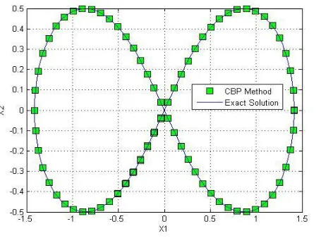
5.3.1 Bernoulli’s lemniscate.

We consider the construction of Bernoulli’s lemniscate by the CBP method. This is a complex curve in a form of a lying figure eight, comprising two loops, which makes it a good example to demonstrate effectiveness of CBP and its advantage over the classical Newton-Raphson method.

The equation of lemniscate in the x1, x2 axes is of the form

𝑓(𝐱) = (𝑥₁2+ 𝑥₂2)2_{− 2𝑎}2_(𝑥

12 − 𝑥22) = 0, 𝑋 = (𝑥1,𝑥2)𝑇 (1)

Using the simplified version of Vorovich-Zipalova’s algorithm, we obtain

𝑓1𝑥̅ 1 + 𝑓2𝑥̅2 = 0 (2)

𝑥̅₁2 _{+ 𝑥̅}

22 = 1 (3)

Where

𝑓₁ = 𝜕𝑓

𝜕𝑥1 = 4𝑥1(𝑥1 2_{+ 𝑥}

22− 𝑎2) (4)

𝑓2 = 𝜕𝑓

𝜕𝑥2= 4𝑥2(𝑥1 2_{+ 𝑥}

22 + 𝑎2) (5)

𝑥̅₁ = 𝜕𝑥1

𝜕𝜎 ; 𝑥̅2 = 𝜕𝑥₂

𝜕𝜎

25

𝑥̅1 = 𝑓2

𝑓12+𝑓22; 𝑥̅2 = −𝑓1

𝑓12+𝑓22 (6)

Starting from the point 𝜎 = 0, 𝑥₁ = 𝑎√2 , 𝑥2 = 0), we proceed iterations

𝑥₁=𝑥₁+ 𝑥̅₁∆𝜎; 𝑥₂=𝑥₂+ 𝑥̅₂∆𝜎 (7)

Figure 1 presents the results of integrating the Cauchy problem with the use of an explicit parameter ‘𝜎’. Figure 2 presents the result obtained by integration according to the classical Newton-Raphson scheme. Unlike the CBP, the Newton-Raphson method is not capable to pass the points with a vertical tangent line where Jacobian turns to zero. The corresponding Matlab code is presented in the appendix.

Figure 2: Application of CBP method (a=1) Figure 3: Application of Newton-Raphson

26

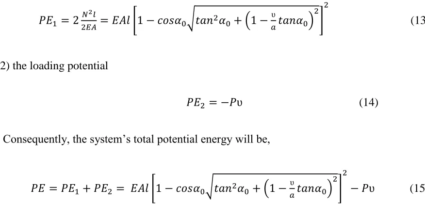
5.3.2 Stability of an imperfect Von Mises Truss

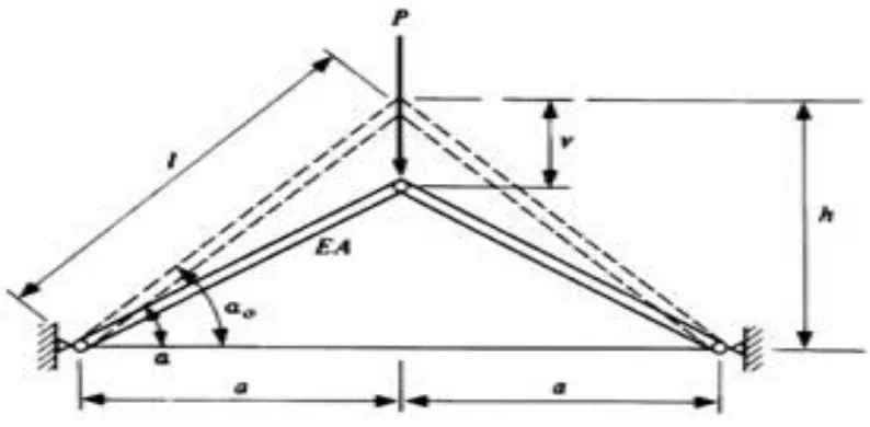
The Von Mises’ truss is a classic example of instability of a geometrically nonlinear mechanical system comprised of perfectly straight elastic bars. The present investigation considers imperfect structures, where each bar is characterized by initial deviation from the straight line. Geometric notation is presented by the Fig.4. Let E – be the Young modulus of the material, w0,w – initial and current maximum values of the bars’ deviation from the straight direction; A,J – the area and moment of inertia of the cross section, Ncr – critical compressing (buckling) force, 𝑁𝑐𝑟 = 𝜋2𝐸𝐽/ 𝑙2, N – the compressive force

Figure 4: Von Misses Truss

The compatibility equation is of the form,

𝑁𝑙

𝐸𝐴+ 𝜋2

4𝑙(𝑤 2_{− 𝑤}

02) = 𝑎 𝑐𝑜𝑠𝛼0−

𝑎

27

The first term on the left of the equal sign quantifies the shortening of the bar due to the

compressive force; the second term – shortening due to the bending of the initially geometrically imperfect bar. The term on the right is the overall change of the length, expressed via geometric parameters.

Introducing critical buckling force into the expression for the normal displacement w,

𝑤 = 𝑤0

1−𝑁 𝑁⁄ 𝑐𝑟 , arrive at the following transcendental equation

𝐹(𝑃, ∝) = 𝑁𝑙

𝐸𝐴+ 𝜋2_𝑤

0 2

4𝑙 [ 1

(1−𝑁 𝑁𝑐𝑟⁄ )2− 1] + 𝑎 𝑐𝑜𝑠𝛼−

𝑎

𝑐𝑜𝑠𝛼0= 0 (2)

where,

𝑁 = 𝑃/(2𝑠𝑖𝑛 ∝)

As it follows from the Figure 4, the vertical displacement of the joint of both bars can be presented as

𝑣 = 𝑎(𝑡𝑎𝑛 ∝₀− tan ∝)

Introducing non-dimensional quantities

𝑁̅ = 𝑁

𝐸𝐴; 𝑃̅ = 𝑃

𝐸𝐴 ; 𝑣̅ = 𝑣

𝑎 ; 𝑎1 = 𝜋2

4 ( 𝑤0

𝑖 ) 2

; 𝑎2 = 𝐴𝑙2

𝜋2_𝐽; (3)

we can present basic equations in the following compact form

𝐹(𝑃̅, ∝) = 𝑁̅ + 𝑎₁[ 1

(1−𝑎2𝑁̅)2− 1] + 𝑐𝑜𝑠𝛼0

𝑐𝑜𝑠𝛼 − 1 = 0 (4)

28

𝑣̅ = 𝑡𝑎𝑛 ∝0− tan ∝ (6)

Using the simplified version of Vorovich-Zipalova algorithm, obtain

𝐹_𝑝𝑃̅_𝜎 + 𝐹_𝛼𝛼̅_𝜎 = 0 (7)

𝑃̅𝜎 2

+ 𝛼̅𝜎 2 = 1 (8)

where

𝐹𝑝 = 𝜕𝐹 𝜕𝑃̅=

𝜕𝐹 𝜕𝑁̅

𝜕𝑁̅

𝜕𝑃̅; 𝐹𝛼 = 𝜕𝐹 𝜕∝ =

𝜕𝐹 𝜕𝑁̅

𝜕𝑁̅

𝜕∝ (9)

𝑃̅ =𝜕𝑃̅

𝜕𝜎; 𝛼̅𝜎 = 𝜕∝̅

𝜕𝜎 (10)

Solution of these equations is presented in the form

𝑃̅_𝜎 = 𝐹𝛼 √𝐹𝑝2+𝐹𝛼2

; 𝛼̅_𝜎 = − 𝐹𝑝 √𝐹𝑝2+𝐹𝛼2

(11)

Starting from the point 𝜎 = 0, 𝑃 = 0 , ∝=∝₀, proceed iterations

𝑃=𝑃 + 𝑃̅𝜎 ∆𝜎; ∝=∝ +𝛼̅𝜎 ∆𝜎 (12)

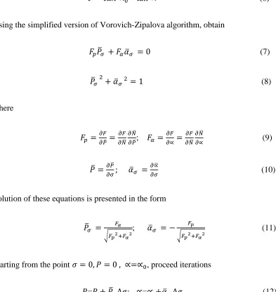
Figure 5 presents the results of integrating the Cauchy problem with the use of an explicit parameter ‘𝜎’. The plot on the top represents the force versus vertical displacement curve which describes equilibrium conditions for the Mises truss. The plot at the bottom shows the total potential energy as a function of displacement.

29

characterizing geometric non-perfectness . The corresponding MATLAB code is presented in the appendix.

Figure 5: The numerical solution of the Von Mises’ Truss showing variation of load P (top)

30

The loading process could be understood from the plot of Figure 5 describing equilibrium condition in terms of a load versus displacement. Let us now suppose that the loading process occurs monotonically from zero (the point zero). It is evident that after the system achieves the state characterized by the point 3, the system should execute a jump immediately to the section III (point 7) on the plot of Figure 5. Two different configurations of the system corresponds to one and the same load 𝑃3 = 𝑃7, i.e., immediately prior to the jump and immediately after it.

Upon further increasing the force P, still higher points of the section III will correspond to equilibrium states of the system.

The process of unloading the system is described by the section III, which starts from some point 8 above point 7 on the same blue curve, and the system’s equilibrium states will be characterized successively by the points 8-7-6-5. If the system is loaded to point 8 and then completely

unloaded to the point 6, the system will not return to its original state. The negative (i.e. upward force) loads P will cause a transition of the system from 6 to 5. Further decreasing the force P (i.e. upon an increase in the load directed upward) the system will complete its reverse jump to the first section (point 2), and then a monotonic process of deformation is established downward along the section I.

The equilibrium points characterized by the points of section II and figure 5 are not realized in the entire process. We are convinced that unstable states correspond to these points. Now it is necessary to discuss the states of the system described by all the points of the horizontal straight line i.e. not only the equilibrium states but also the non-equilibrium states.

31

1) the potential energy of the deformation, which we can specify by equation

𝑃𝐸1 = 2 𝑁2𝑙

2𝐸𝐴 = 𝐸𝐴𝑙 [1 − 𝑐𝑜𝑠𝛼0√𝑡𝑎𝑛

2_𝛼

0+ (1 −

ʋ

𝑎𝑡𝑎𝑛𝛼0) 2

] 2

(13)

2) the loading potential

𝑃𝐸₂ = −𝑃ʋ (14)

Consequently, the system’s total potential energy will be,

𝑃𝐸 = 𝑃𝐸₁+ 𝑃𝐸₂ = 𝐸𝐴𝑙 [1 − 𝑐𝑜𝑠𝛼₀√𝑡𝑎𝑛2_𝛼

0+ (1 −

ʋ

𝑎𝑡𝑎𝑛𝛼0) 2

] 2

− 𝑃ʋ (15)

The relationship between the total potential energy and the vertical displacement is shown in figure 5 with the red plot (bottom figure).

Now the stability of each point on the curve could be understood by the total potential energy curve. Suppose we are given 3 points A, B and C on the force versus displacement curve. These 3 points A, B and C corresponds to the same load ‘P’. Now we plot the total potential energy curve for the corresponding load ‘P’ and position our points A, B and C accordingly. As per the theory suggests, the points with lower potential energy are stable whereas the points with higher potential energy are unstable. Now looking at the plot, we see points A and C have lower

32

The classical Newton-Raphson method being applied to the bifurcation Mises truss problems diverges, since Jacobian turns zero at the extreme points.

Figure 6: The solution of the Von Mises’ Truss showing the variation of equilibrium curves

33

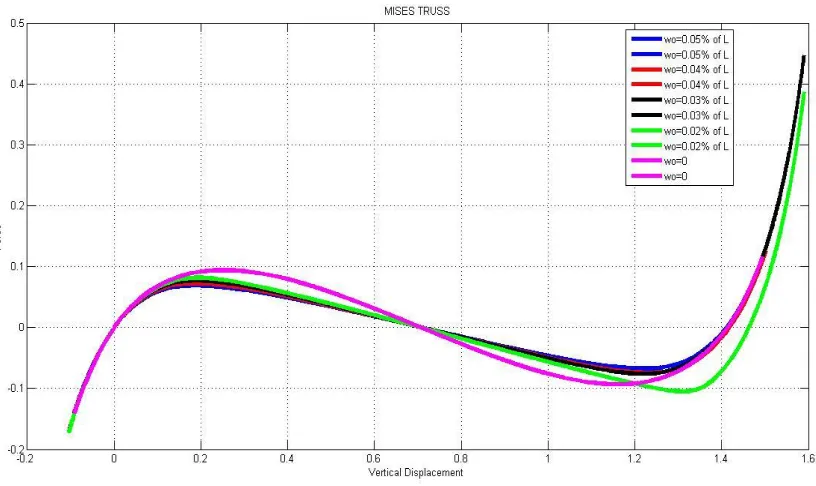
5.3.3 Equilibrium composition of a gas mixture at high temperature

The theoretical determination of equilibrium compositions in the flow of chemically reacting fluids is complicated by the fact that it is necessary to obtain the simultaneous solutions of a system of nonlinear algebraic equations. Let us consider a one mole of CO2 at 10 atm which is heated in a steady-flow constant pressure process. It is required to find the equilibrium

compositions at a total pressure of 10 atm and a range of temperature from 1000 to 6000 K. The equilibrium composition is assumed to consist of CO2, CO, and O2, and is characterized by the unknown constants α, β and γ - the number of moles, as shown by the following balance equation

𝐶𝑂2 → 𝛼𝐶𝑂2+ 𝛽𝐶𝑂 + 𝛶𝑂2 (1)

For the balance equations we can write:

-according to the balance of element C:

𝛼 + 𝛽 = 1 (2)

-according to the balance of the element O

2𝛼 + 𝛽 + 2𝛶 = 2 (3)

According to the statement of a law of mass action

𝛽√𝛶 𝛼

1

√𝛼 + 𝛽 + 𝛶√𝑃𝑟 = 𝐾

34

𝛽2𝛾𝑃_𝑟− 𝐾2𝛼2(𝛼 + 𝛽 + 𝛾) = 0 (4)

Where K – is the equilibrium constant, 𝑃_𝑟 – total pressure, given by the attached table

Introduce parameter of continuation p as the following

∝ +𝛽 − 1 = (1 − 𝑝)(∝₀+ 𝛽₀− 1) (5)

2 ∝ +𝛽 + 2𝛾 − 2 = (1 − 𝑝)(2 ∝0+ 𝛽0+ 2𝛾0 − 2) (6)

𝛽2_𝛾𝑃

𝑟− 𝐾2 ∝2 (∝ +𝛽 + 𝛾) = (1 − 𝑝)(𝛽02𝛾0𝑃𝑟− 𝐾2 ∝02 (∝0+ 𝛽0+ 𝛾0) (7)

Where mole numbers marked by zero indices, are the relating initial approach, all chosen as 0.5

Differentiating by parameter, arrive to the following system

𝐴𝑉 = 𝑅 (8)

where,

𝐴 = [

1 1 0

2 1 2

−𝐾2(3 ∝2+ 2 ∝ 𝛽 + 2 ∝ 𝛾) 2𝛾𝛽𝑃𝑟− 𝐾2 ∝2 𝛽2𝑃𝑟− 𝐾2 ∝2

] (9)

35

𝑉 = ⌈𝑑∝_𝑑𝑝 𝑑𝛽_𝑑𝑝 𝑑𝛾_𝑑𝑝⌉𝑇 (11)

Starting from the point 𝑝 = 0, 𝑃𝑟 = 0 , ∝= 𝛽 = 𝛾 = 0.5, proceed iterations until 𝑝 = 1

𝑉= 𝑉 + 𝐴−1𝑅∆𝑝;

Figure 7 tracks evolution of mole coefficients during integration of the Cauchy problem with the use of an explicit parameter ‘𝑝’. The final results are practically the same obtained in [13]. The relating MATLAB based text code is presented in the attachment.

36

5.4Nonlinear problems described by the system of ODE

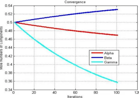
5.4.1 Blasius Solution in the Boundary Layer Theory

We present the basic idea of application of a CBP method to ODE based on Blasius boundary value problem.

Figure 8: Boundary layer over the plate

Consider the flow of an incompressible fluid over a semi-infinite flat plate, as shown in Fig. 8. By introducing the boundary layer assumptions (i.e., the existence of a very thin layer), the Navier-Stokes equations becomes,

𝜕𝑢 𝜕𝑥+

𝜕𝑣 𝜕𝑥 = 0

(1)

𝑢𝜕𝑢

𝜕𝑥+ 𝑣

𝜕𝑢

𝜕𝑦 = 𝑣

37

subject to the boundary conditions

𝑦 = 0; 𝑢 = 𝑣 = 0

(2)

𝑦 = ∞; 𝑢 = 𝑈_∞

Blasius introduced the following transformation

𝑢 =𝜕𝛹

𝜕𝑦, 𝑣 = − 𝜕𝛹

𝜕𝑥 (3)

𝜂 = 𝑦√𝑈∞

𝑣𝑥

(4)

𝑓(𝜂) = 𝛹/√𝑣𝑥𝑈∞

which transform the N-S equations to,

𝑑

3_𝑓

𝑑𝜂3+ 1 2𝑓

𝑑2𝑓

𝑑𝜂2 = 0 (5)

subject to the boundary conditions

𝑓(0) =𝑑𝑓(0)

𝑑𝜂 = 0,

𝑑𝑓(∞)

𝑑𝜂 = 1

The following algorithm is presented as a sequence of steps:

Step 1: Present BVP in a canonical form as a system of the 1st _{order ODE}

38

𝐹₃′= −0.5𝐹1𝐹3, 𝐹1(0) = 0 (6)

𝐹₂′= 𝐹₃, 𝐹₂(0) = 0 (7)

𝐹₁′= 𝐹₂; 𝐹₂(∞) = 1 (8)

Step 2: Introduce parameter p, and imbed obtained ODE in a p –parametric family

𝐹₃′= −0.5[(𝐹1− 1)𝑝 + 1]𝐹3, 𝐹1(0) = 0 (9)

𝐹₂′= 𝐹₃, 𝐹₂(0) = 0 (10)

𝐹₁′= 𝐹₂; 𝐹₂(∞) = 1 (11)

Step 3: Obtain initial conditions at 𝒑 = 𝟎,

𝐹3 = 0.5𝑒−𝜂/2 (12)

𝐹₂ = 1 − 𝑒−𝜂/2 (13)

𝐹₁ = 𝜂 − 2(1 − 𝑒−𝜂2) ₍₁₄₎

Step 4:Differentiating by parameter ‘𝒑’, arrive at the following system with respect to

sensitivities to the parameter 𝒑,

𝑉′= 𝐴𝑉 + 𝑅, (15)

Where

𝐴 = [

0 1 0

0 0 1

−0.5𝑝𝐹3 0 −0.5(𝑝𝐹3+ 1)

] ; 𝑅 = [

0 0

−0.5𝐹3(𝐹1− 1)

39

𝑉 =𝑑𝐹

𝑑τ; 𝐹 = [ 𝐹₁ 𝐹2 𝐹₃

] (17)

Step 5: Apply superposition principle and specify Cauchy problem for each component

𝑉 = 𝑎𝑈 + 𝑊 (18)

Where U,W – unknown vector functions; a – unknown “blend” coefficient

Solving the following two Cauchy problems for each component

𝑈′= 𝐴𝑈; 𝑈(0) = [ 0 0 1

] (19)

𝑊′= 𝐴𝑊 + 𝑅; 𝑊(0) = [ 0 0 0

] (20)

we satisfy then automatically to the original ODE

(𝑎𝑈 + 𝑊)′_{= 𝐴(𝑎𝑈 + 𝑊) + 𝑅 (21)}

Or

(𝑎𝑈′− 𝐴𝑈) + (𝑊′− 𝐴𝑊 − 𝑅) = 0 (22)

and left boundary conditions.

Step 6: Solution of the Cauchy problems

Numerical scheme used in this work, is an implicit scheme, presented in the following form (I –

identity matrix)

𝑈𝑖+1−𝑈𝑖

Δ𝜂 = 𝐴𝑈

40

𝑊𝑖+1−𝑊𝑖

Δ𝜂 = 𝐴𝑊

𝑖+1_{+ 𝑅; 𝑜𝑟 (𝐼 − Δ𝜂𝐴)𝑊}𝑖+1_{= 𝑊}𝑖 _{+ Δ𝜂𝑅 (24)}

wherefrom,

𝑈𝑖+1_{= (𝐼 − Δ𝜂𝐴)}−1_𝑈𝑖 ₍₂₅₎

𝑊𝑖+1_{= (𝐼 − Δ𝜂𝐴)}−1_(𝑊𝑖 _{+ Δ𝜂𝑅) (26)}

Step 7: Satisfy to the right BC by choosing the corresponding “blend” coefficient

Since the original right BC is applied only for the function F2 , as F2=1, solving ODE for sensitivities we need to apply V2=0, which in matrix form looks as (J=[0 1 0] )

𝐽 ∗ 𝑉 = 0, 𝑜𝑟 𝐽 ∗ (𝑎𝑈 + 𝑊) = 0 (27)

wherefrom, 𝑎 = −𝐽∗𝑊

𝐽∗𝑈 (28)

41

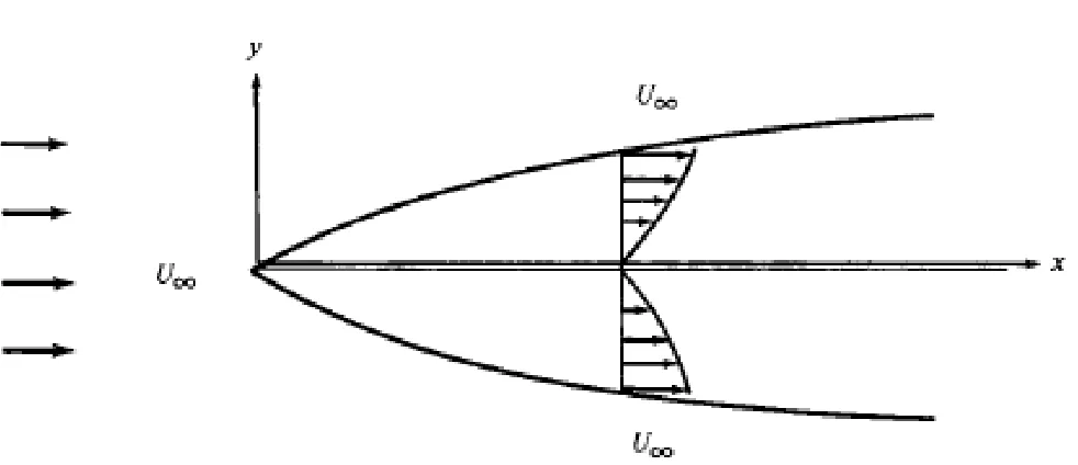
42

5.4.2 Faulkner-Skan Solution of the Boundary Layer Flow over Wedges

Figure 10: Boundary Layer Flow around the Wedge

We will now apply the method of parameter differentiation to the boundary layer equations governing the flow of fluids over the wedge as shown in Fig.10. The governing differential equations, derived from the Navier-Stokes equations, are identical to equations presented in section 5.4.1 except for an additional term, resulting from the fact that the mainstream velocity, i.e. the velocity at the edge of the boundary layer, is now a function of x. Similar to the Blasius equation, which derivation is based on a similarity transformation, the Falkner-Skan equation results in

𝑑𝑒𝑓 𝑑𝜂3+ 𝑓

𝑑2𝑓

𝑑𝜂2+ 𝛽 [1 − ( 𝑑𝑓 𝑑𝜂)

2

43

subject to the boundary conditions

𝜂 = 0; 𝑓 = 0, 𝑑𝑓 𝑑𝜂= 0

(2)

𝜂 = ∞; 𝑑𝑓

𝑑𝜂 = 1

where ‘β’ relates to the power of a flow velocity profile. Solution of this equation has attracted the attention of both applied mathematicians and aeronautical engineers.

The mathematical algorithm of solving the Falkner-Skan equation is very similar to the one used for the solution of a Blasius boundary layer model, and is not presented here. Fig. 11 presents distribution of an axial velocity (non-dimensioned) as a function of a normal distance to the wall for different β. Distributions are in an excellent agreement with results presented in [37]. The corresponding MATLAB based text code is presented in Appendix.

44

5.4.3 Rotating Disc Boundary Layer Flow

Figure 12: Flow over a rotating disc

The flow due to the rotating disc in a viscous fluid, as shown in the figure 12, was originally solved by Von Karman [32]. The original problem definition is available in Schlichting [32]. A disk of radius R is rotating with an angular velocity ω in still fluid. The flow is steady,

45

the dimensionless functions F, G and H, and an equation for the dimensionless dynamic pressure P in the fluid above the disk [33]:

2𝐹 + 𝐻̇ = 0

𝐹2+ 𝐹̇𝐻 − 𝐺2− 𝐹̈ = 0

(1)

2𝐹𝐺 + 𝐻𝐺̇ − 𝐺̈ = 0

𝑃̇ + 𝐻𝐻̇ − 𝐻̈ = 0

The following boundary conditions supplement the ODE system (1),

𝜂 = 0 ; 𝐹 = 0; 𝐺 = 1; 𝐻 = 0; 𝑃 = 0

(2)

𝜂 = ∞ ; 𝐹 = 0; 𝐺 = 0

46

E.M. Sparrow and J.J Gregg values

CBP method values (Coarse Mesh-100 cells)

CBP method values (Fine Mesh-3500 cells)

η Ḟ −Ġ −Ḣ Ḟ −Ġ −Ḣ Ḟ −Ġ −Ḣ

0 0.510 0.6159 0 0.5284 0.6216 0 0.5133 0.6189 0

∞ 0 0 0.8845 0.0001 0.0001 0.8644 0.0001 0.0001 0.8859

Time for convergence of solution 2.3 seconds 65 seconds

Table 1: Shows the comparison of the solution values obtained by E.M. Sparrow and J.J.

Gregg, and the values obtained by the proposed CBP method.

The graphical representations of these results are shown below. Results were compared with the published results obtained by Schlichting and the results obtained using Bezier functions to solve the differential equation with the given boundary conditions [32]. Figure 13 shows the

comparison between CBP method results and results presented by Schlichting [32].

Figure 13: The plot shows the comparison for velocity distribution between the results

47

5.4.4 General Solution for Troesch's Problem

Troesch' problem is an excellent example for testing different numerical schemes. Originally derived to predict the confinement of a plasma column, it serves as a difficult testing case for different algorithms. The continuation by parameter method is employed to obtain the solution for the nonlinear differential equation which describes Troesch’s problem. In contrast to other reported solutions obtained by various methods, the proposed solution shows the highest degree of accuracy in the results for a remarkable wide range of values of Troesch’s parameter.

Troesch's boundary value problem, in terms of dimensionless variables can be written as:

𝑑2𝑦

𝑑𝑥2 = 𝑛 sinh 𝑛𝑦 (1)

subject to the boundary conditions

𝑦(0) = 0, 𝑦(1) = 1 (2)

Following the described procedure relating to the CBP method, we present equation (1) in a form of a system of two nonlinear equations of the first order.

𝑦′_{= 𝑧}

𝑧′ _{= 𝑛 sinh 𝑛𝑦}

Differentiating with parameter ‘n’ results in the following “sensitivity” equations

𝑦̅ =𝑑𝑦

𝑑𝑛; 𝑧̅ = 𝑑𝑧 𝑑𝑛

𝑦̅′_{= 𝑧̅}

48

being supplemented by the boundary conditions,

𝑦̅(0) = 0; 𝑦̅(1) = 0

Following stepwise procedure and updating the solution for incrementally increased parameter ‘n’ provides a single step solutions which looks as,

𝑦(𝑛 + 𝑑𝑛) = 𝑦(𝑛) + 𝑦̅∆𝑛

𝑧(𝑛 + 𝑑𝑛) = 𝑧(𝑛) + 𝑧̅∆𝑛

In matrix form, 𝑉̅′ _{= 𝐴𝑉̅ + 𝐹}

𝑉 = (𝑦_𝑧) 𝑉̅ = (𝑦̅ 𝑧̅)

𝐴 = ( 0 1

𝑛2cosh 𝑛𝑦 0) ; 𝐹 = (

0

sinh 𝑛𝑦 + 𝑛𝑦 cosh 𝑛𝑦)

Furthermore,

𝑉(𝑛 + ∆𝑛) = 𝑉(𝑛) + 𝑉̅∆𝑛 (3)

Easy to see that the large number for ‘n’ correspond to the steep edge effect at the right boundary condition for the presented nonlinear BVP. Troesch [34] and Ehrlich [35] pointed out that this two-point boundary value problem is unstable and difficult to solve. Roberts and Shipman [36] suggested that the equation can be solved by combination of three different methods, namely, the perturbation technique, the parallel shooting method, and the continuation method. The

49

n=1

50

Figure 14: The figure shows the solution of Troesch’s equation using Wolfram

Mathematica for n=1, n=2, n=3 and n=4 respectively

n=3

51

52

Figure 15: The figure shows the solution of Troesch’s equation using MatLab for n=1 and

53

The MATLAB’s ODE toolbox was also used to solve the Troesch’s equation. As compared to the solution obtained by Mathematica, the solution obtained using MATLAB was stable for lower parametric values but as the parametric values goes above 2, the program crashes and MATLAB is unable to provide any results. We can see that it is really difficult to obtain a solution for large parametric values.

Figure 16: The figure shows the solution of Troesch’s equation using continuation by

54

An efficient algorithm based on the continuation by parameter method has been successfully applied to Troesch’s problem which provides the stable solutions for higher values of parameter ‘n’. As it can be seen from the figure 17, the continuation by parameter provides us a stable solution for a parametric value up to n=100. It is important to emphasize that for the first time in the literature of the Troesch’s problem, the solution is plotted for large values of n=100.

5.5An Alternative Formulation of Bellman’s Method of Invariant Imbedding

The classical invariant imbedding is based on a partitioning of an interval of integration, with a following integration across each partition [3], [4], [5], [6].

We suggest a modification based on an introduction of a parameter of continuation, which is a range of integration of a relating BVP, varying from zero to the nominal value

𝑑𝑌

𝑑𝑥 = 𝐹(𝑥, 𝑌); 𝑥 = 𝑥̅𝑙; 𝑌̂ = 𝑑𝑌

𝑑𝑙 - sensitivities to the length change

𝑑𝑌

𝑑𝑥̅ = 𝑙𝐹(𝑥, 𝑌); 𝑙=0 – corresponds to initial approach

Linear equation for the vector of sensitivities 𝑑𝑌̂

𝑑𝑥̅− 𝑙𝐹𝑌𝑌̂ = 𝐹 + 𝑙𝐹𝑥𝑥̅

Solution update

55

Discrete counterpart can be suggested as well. Approximating original ODE by finite difference equation of a second order of accuracy, obtain

𝑦𝑖−1− 2𝑦𝑖+ 𝑦𝑖+1

𝐿2 𝑁2 = 𝑛sinh (𝑛𝑦𝑖)

Or

𝑦_𝑖−1− 2𝑦_𝑖+ 𝑦_𝑖+1= 𝑙

𝑁2 𝑛sinh (𝑛𝑦𝑖), 𝑙 = 𝐿2

Introducing derivatives by 𝑙, 𝑑𝑦

𝑑𝑙 = 𝑦̅, rewrite basic equations in terms of sensitivities to the span

variation

𝑦𝑖−1

̅̅̅̅̅ − 2𝑦̅ + 𝑦𝑖 ̅̅̅̅̅ =𝑖+1 𝑙

𝑁2 𝑛[sinh(𝑛𝑦𝑖) + 𝑙𝑐𝑜𝑠ℎ(𝑛𝑦𝑖)𝑛𝑦̅𝑖],

The final tri-diagonal system that is one with a bandwidth of 3 can be expressed as

𝑎𝑦̅_𝑖−1+ 𝑏𝑦̅_𝑖 + 𝑐𝑦̅_𝑖+1= 𝑟_𝑖

𝑎 = 𝑐 = 1; 𝑏 = −2 − (𝑛 𝑁)

2

𝑙𝑐𝑜𝑠ℎ(𝑛𝑦_𝑖); 𝑟 = 𝑛

𝑁2𝑠𝑖𝑛ℎ(𝑛𝑦𝑖)

Solution of obtained tridiagonal equations is obtained by the Thomas method. Updated solution is given as,

𝑦_𝑖 = 𝑦_𝑖 + 𝑦̅_𝑖∆𝑙, i=1,…, N.

At initial point, when span is equal to zero, solution is a linear interpolation of boundary values inside domain, i.e. 𝑦_𝑖 = 𝑖−1

56

Figure 17: The figure shows the solution of Troesch’s equation using invariant imbedding

57

6.

CONCLUSION

Continuation by parameter method has been applied to different nonlinear boundary value problems from different areas of engineering like fluid mechanics, mechanics of solid, stability, etc.

58

7.

REFERENCES

[1]. Ambarzumian, V. A., "Theoretical Astrophysics," Pergamon, Oxford, 1958. [2]. Chandrasekhar, S., "Radiative Transfer," Dover, New York, 1960.

[3]. Arosesty, J., Bellman, R., Kalaba, R., and Ueno, S., Invariant imbedding and rarefied gas dynamics, Proc. Natl. Acad. Sci. 50,222 (1963).

[4]. Bellman, R., Kalaba, R., and Prestrud, M. C., "Invariant Imbedding and Radiative Transfer in Slabs of Finite Thickness," American Elsevier, New York, 1963.

[5]. Bellman, R., Kagiwada, H. H., Kalaba, R. E., and Prestrud, M. c., "Invariant Imbedding and Time-Dependent Transport Processes," American Elsevier, New York, 1964.

[6]. Bellman, R., and Kalaba, R. E., Invariant imbedding, random walk, and scattering, J. Math. Mech. 9, 411 (1960).

[7]. Bellman, R., and Kalaba, R. E., Wave branching processes and invariant imbedding,

Proc. Natl. Acad. Sci. 47, 1507 (1961).

[8]. Bellman, R., and Kalaba, R. E., A Note on Hamilton's equations and invariant imbedding, Q. Appl. Math. 21, 166 (1963).

[9]. Wing, G. M., "An Introduction to Transport Theory," Wiley, New York, 1962. [10]. Lee, E. S., "Quasilinearization and Invariant Imbedding," Academic Press, New York, 1968.

[11]. Meyer, G. H., "Initial Value Methods for Boundary Value Problems," Academic Press, New York, 1973.

59

Equations: An Introduction," Addison-Wesley, Reading, Massachusetts, 1973. [13]. Na T.Ya. Computational methods in boundary value problems. Mathematics in science and engineering. Volume 145. 1979

[14]. Grigolyuk E.I.,Shalashilin V.I. Problems of nonlinear deformation. 1991 [15]. Ortega, J.M.,Rheinboldt, W.C., “Itertaive Solution of Nonlinear Equations in Several Variables”, Academic Press. New Ypork – London, 1970

[16]. Bittner, L. ISNM, International Series of Numerical Mathematics, Vol. 7, Verlag, Basel, SHttgart (1987), pp.114-135

[17]. Distefano, N., Todeschini, R. A quasolinearization approach to the solution of elastic beams on nonlinear foundations, Int. J. Solids Struct, 11,No 1, 89-97, 1975 [18]. El-Zanaty, M.H., Murray D.W. Non linear finite element analysis of steel frames, J.Struct Eng., 109, 2, 353-368, 1983

[19]. Vorovich I.I.,Zipalova, V.F. Solution of nonlinear boundary value problems by passing to a Cauchy problem. Applied Mathematics and Mechanics., 29, N4, 357-367, 1965

[20].On the numerical solution of snapping problems in the theory of elastic stability. Sudaar #410, Stanford, CA, 1982

[21]. Ricks, An incremental approach to the solution of snapping and buckling problems. Int. J. Solids Structures 15,524-551 (1979).

[22]. Ricks, E. The application of Newton’s method to the problem of elasticity, Trans. ASME J.Appl Mech, E39, No4, 1060-1065, 1972

60

[24]. Waszczyszyn, Z Numerical problems of nonlinear stability analysis. Comput. Structures, 17, No 1, 69-72, 1983

[25]. Watson , L.T., Holzer, S.M. Quadratic convergence of Crisfield’s method. Comput. Structures, 17. No1, 69-72, 1983

[26]. Walker A.S., Hall D.G. AN analysis of the large deflection of beams using finite element method. Aeronaut. Quart., 19. No4, 357-367, 1968

[27]. Weinitschke H.J., On the calculation of limit and bifurvation points in stability problems of elastic shells. Int, J. Solid. Struct, 24, No1, 79-85, 1985

[28]. Valli, A. M., Elias, R. N., Carey, G. F., & Coutinho, A. L. (2009). PID adaptive control of incremental and arclength continuation in nonlinear applications. International Journal for Numerical Methods in Fluids Int. J. Numer. Meth. Fluids, 61(11), 1181-1200. doi:10.1002/fld.1998

[29]. Keller H.B. Numerical solution of bifurcation and nonlinear eigenvalue problems. In P.H.Rabinowitz, Application of bifurcation theory, 359-384, Academic Press, NY, 1977

[30]. Stability and oscillation of elastic systems: Modern concepts, paradoxes and errors : Panovko, Y. G. : Free Download & Streaming : Internet Archive. (n.d.). Retrieved March 10, 2016, from https://archive.org/details/nasa_techdoc_19740006513

61

[33]. Venkataraman, P. (n.d.). Explicit Solutions for Differential equations. Retrieved March 10, 2016, from https://people.rit.edu/~pnveme/ExplictSolutions2/ Explicit Solutions to Differential Equations, Flow over a Rotating Disk

[34]. B.A. Troesch, Intrinsic difficulties in the numerical solution of a boundary value problem, Internal Report NN–142, TRW Inc., Redondo Beach, California, 1960

[35]. L. EHRLICH, Experience with Numerical Methods for a Boundary Value Problem, Internal Report NN-141, TRW Inc., Redondo Beach, Calif., 1960

62

A.

APPENDIX

MATLAB Computer Text Codes

Bernoulli Lemniscate

1. clc; clear all; close all

2. %Plot Bernoulli Lemniscate

3. x1=sqrt(2); x2=0;

4. AX1(1)=x1; AX2(1)=x2; tau=0.00001; a=1; 5.

6. for i=2:1000000

7. J1=(x1^2+x2^2)*x1-a^2*x1; 8. J2=(x1^2+x2^2)*x2+a^2*x2; 9. J=sqrt(J1^2+J2^2);

10. x1=x1+tau*J2/J; x2=x2-tau*J1/J; 11. AX1(i)=x1; AX2(i)=x2;

12.end

13.%Filter points for plotting

14.k=0;

15.for i=1:10000:1000000 16. k=k+1;

17. X(k)=AX1(i); Y(k)=AX2(i); 18.end

19.% plot(AX1,AX2); grid on; xlabel('X1'); ylabel('X2');

63

21.plot(X,Y,'rs','MarkerEdgeColor','k',...

22. 'MarkerFaceColor','g',...

23. 'MarkerSize',10) 24.%Exact solution

25.t=linspace(0,2*pi);

26.X=a*sqrt(2)*cos(t)./(1+sin(t).^2); 27.Y=a*sqrt(2)/2*sin(2*t)./(1+sin(t).^2); 28.hold on

29.plot(X,Y);

30.grid on; xlabel('X1'); ylabel('X2'); 31.legend('CBP Method','Exact Solution') 32.

33.%Newton=-Raphson

34.

35.x=-sqrt(2); y=1; 36.for ii=1:101 37. for k=1:100

38. F=(x^2+y^2)^2-2*a^2*(x^2-y^2); 39. DFY=4*((x^2+y^2)*y+a^2*y); 40. DY=F/DFY;

41. y=y-DY;

64

44. break

45. end ; 46. end%k

47. XN(ii)=x; YN(ii)=y; 48. ii,x=x+2*sqrt(2)/100 49.end%ii

50.figure

51.plot(XN,YN,'rs','MarkerEdgeColor','k',...

52. 'MarkerFaceColor','g',...

53. 'MarkerSize',10); 54.hold on

55.plot(X,Y);

56.grid on; xlabel('X1'); ylabel('X2'); 57.

65

Gas mixture composition

%Equilibrium Mixture

clc; close all; clear all

Ntau=100; %number of intervals

dtau=1/Ntau; TAU=0:dtau:1;

al=0.5; bt=0.5; gm=0.5;

AL(1)=al; BT(1)=bt; GM(1)=gm; K=exp(0.61); p=10; V=[al bt gm ]; %Initial vector at tau=0

A(1,1)=1; A(1,2)=1; A(1,3)=0; A(2,1)=2; A(2,2)=1; A(2,3)=2;

for i=1:Ntau F(1)=-(al+bt-1);

F(2)=-(2*al+bt+2*gm-2);

F(3)=K^2*al^2*(al+bt+gm)-bt^2*gm*p;

A(3,1)=-K^2*(3*al^2+2*al*bt+2*al*gm); A(3,2)=2*bt*gm*p-K^2*al^2

66

DV=A\F'; V=V+DV'*dtau; %Updated

al=V(1); bt=V(2); gm=V(3);

AL(i+1)=al; BT(i+1)=bt; GM(i+1)=gm;

end

V

plot(AL,'--rs','LineWidth',2,...

'MarkerEdgeColor','k',...

'MarkerFaceColor','r',...

'MarkerSize',10) hold on

plot(BT,'--bd','LineWidth',2,...

'MarkerEdgeColor','k',...

'MarkerFaceColor','b',...

'MarkerSize',10) hold on

plot(GM,'--cd','LineWidth',2,...

'MarkerEdgeColor','k',...

'MarkerFaceColor','g',...

67

title('Mole Coefficients. Convergence ') grid on

legend('Alpha','Betta','Gamma') xlabel('Iterations')

68

Blasius Boundary Layer Model

% Solving Blasius BV problem:

%f'''+0.5*f*f''=0; f(0)=f'(0)=0; f'(inf)=1;

clc; close all; clear all

N=100; %number of layers from eta=0 to eta=10 (inf)

Ntau=100; %number of tau imcrements

dtau=1/Ntau; deta=10/N;

%Exact solution of a simplified model at initial state (tau=0)

ETA=linspace(0,10,N+1); F3=0.5*exp(-ETA/2); F2=1-exp(-ETA/2);

F1=ETA-2*(1-exp(-ETA/2)); plot(ETA,F2,'LineWidth',2) hold on

tau=0;

for itau=1:Ntau

U=[0;0;1]; %initial conditions for sensitivities

W=[0;0;0];

AU(1,:)=U; AW(1,:)=W;

for i=1:N %integrate eq for sensitivities U and W

69

M=[0 1 0; 0 0 1; -tau*F3(i)/2 0 -(tau*(F1(i)-1)+1)/2]; R=[0;0;-F3(i)*(F1(i)-1)/2];

DINV=inv(eye(3)-deta*M); U=DINV*U;

W=DINV*(W+deta*R); AU(i+1,:)=U; AW(i+1,:)=W; end%i

%Blend coefficient

A=-W(2)/U(2);

%Total vector of sensitivities

AV=A*AU+AW;

%Update F functions

F1=F1+dtau*AV(:,1)'; F2=F2+dtau*AV(:,2)'; F3=F3+dtau*AV(:,3)'; tau=tau+dtau;

end %itau

70

grid on

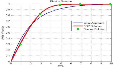
xlabel('ETA'); ylabel('Axial Velocity'); title('Blasius Solution')

hold on

XX=[ETA(10), ETA(30), ETA(50), ETA(70), ETA(100)]; YY=[F2(10), F2(30), F2(50), F2(70), F2(100)];

plot(XX,YY,'bd',...

'MarkerEdgeColor','k',...

'MarkerFaceColor','g',...

'MarkerSize',10)

71

Falkner-Skan Flow across the edge

% Solving Falkner-Skan BV problem:

clc; close all; clear all

N=100; %number of layers from eta=0 to eta=10 (inf)

Ntau=100; %number of tau imcrements

dtau=1/Ntau; deta=4/N;

b=-0.3; b=0; b=0.3; b=0.6

for ib=1:5

b=-0.3+(ib-1)*0.3;

% for b=-0.3:0.3:1.2 %-0.3:0.3:0.6

%Exact solution of a simplified model at initial state (tau=0)

ETA=linspace(0,4,N+1); F3=exp(-ETA);

F2=1-exp(-ETA);

F1=-1+ETA+exp(-ETA );

72

% hold on

tau=0;

for itau=1:Ntau

U=[0;0;1]; %initial conditions for sensitivities

W=[0;0;0];

AU(1,:)=U; AW(1,:)=W;

for i=1:N %integrate eq for sensitivities U and W

M=[0 1 0; 0 0 1; -tau*F3(i) 2*tau*b*F2(i) -(tau*(F1(i)-1)+1)]; R=[0;0;-F3(i)*(F1(i)-1)+b*(F2(i)^2-1)];

DINV=inv(eye(3)-deta*M); U=DINV*U;

W=DINV*(W+deta*R); AU(i+1,:)=U; AW(i+1,:)=W; end%i

%Blend coefficient

A=-W(2)/U(2);

73

AV=A*AU+AW;

%Update F functions

F1=F1+dtau*AV(:,1)'; F2=F2+dtau*AV(:,2)'; F3=F3+dtau*AV(:,3)'; AF2(:,ib)=F2;

end %itau

% get(0,'DefaultAxesColorOrder');

% plot(ETA,F2,'r','LineWidth',3)

% hold on

end

get(0,'DefaultAxesColorOrder'); plot(ETA,AF2,'LineWidth',2); legend('b=-3','b=0','b=0.3','b=0.6')

ylabel('Scaled Axial Velocity'); xlabel('Scaled Distance From the Wall')

grid on

74

Stability of an imperfect Von Mises’ truss

clc; clear all; close all

%Input Data

%==========

L=1; AL0=pi/4; a=L*cos(AL0); w0=0; tan0=tan(AL0); cos0=cos(AL0); a1=(pi*w0/(2*L))^2;

A=0.5^2; J=0.5^4/12; a2=A*L^2/(pi^2*J);

%Initial data

AL(1)=AL0; AP(1)=0; V(1)=0;%displacement

dsig=0.001;

for i=2:1800 %Derivatives

s=sin(AL(i-1)); c=cos(AL(i-1)); p=AP(i-1); FP=1+2*a1*a2*s^3/(s-a2*p)^3; %Derivative by P

NUM1=3*s^2*c*(s-a2*p)^2; NUM2=s^3*2*(s-a2*p)*c; DEN=(s-a2*p)^4;

75

ALD=-FP/sqrt(FP^2+FAL^2); PD=FAL/sqrt(FAL^2+FP^2); AL(i)=AL(i-1)+ALD*dsig; AP(i)=AP(i-1)+PD*dsig; V(i)=L*(sin(AL0)-s);

end

plot(V,AP,'linewidth', 4); grid on

xlabel('Vertical Displacement'); ylabel('Force'); title('MISES TRUSS')

hold on % clear V AP

AP1(1)=0; V1(1)=0;%displacement

EE(1)=0; %potential energy in the absense of load for i=2:200

%Derivatives

s=sin(AL(i-1)); c=cos(AL(i-1)); p=AP1(i-1); FP=1+2*a1*a2*s^3/(s-a2*p)^3;

76

DEN=(s-a2*p)^4;

FAL=a1*(NUM1-NUM2)/DEN+cos(AL0)/c^2-c; ALD=FP/sqrt(FP^2+FAL^2);

PD=-FAL/sqrt(FAL^2+FP^2); AL(i)=AL(i-1)+ALD*dsig; AP1(i)=AP1(i-1)+PD*dsig; V1(i)=L*(sin(AL0)-s);

end

plot(V1,AP1,'linewidth', 4); grid on

hold on

%Total Potential energy

%=============================

for i=2:1800 %Derivatives

s=sin(AL(i-1)); c=cos(AL(i-1)); p=AP(i-1); FP=1+2*a1*a2*s^3/(s-a2*p)^3; %Derivative by P

NUM1=3*s^2*c*(s-a2*p)^2; NUM2=s^3*2*(s-a2*p)*c; DEN=(s-a2*p)^4;

FAL=a1*(NUM1-NUM2)/DEN+cos(AL0)/c^2-c; %derivative by ALFA

77

PD=FAL/sqrt(FAL^2+FP^2); AL(i)=AL(i-1)+ALD*dsig; AP(i)=AP(i-1)+PD*dsig; V(i)=L*(sin(AL0)-s); %Potential energy

Pbar=0.1;

EE(i)=(1-cos0*sqrt(tan0^2+(1-V(i)/a*tan0)^2))^2-Pbar*V(i)/L;

end

plot(V,EE,'r','linewidth',4); grid on

78

Rotating Disc Boundary Layer Flow

% Solving Flow around Rotating disk

clc; close all; clear all

N=100; %number of layers from eta=0 to eta=10 (inf)

Ntau=200; %100; %number of tau imcrements

L=10; %length

dtau=1/(Ntau-1); %step n load increments

deta=L/N;

% at initial state (tau=0)

ETA=linspace(0,10,N+1);

%Vectors initialization

X1=zeros(N+1,1); X2=zeros(N+1,1); X3=zeros(N+1,1); %X3(1)=tau - corrected inside loop

X4=zeros(N+1,1); X5=zeros(N+1,1); P=zeros;

%Sensitivities (bar variables)

X1B=zeros(N+1,1); X2B=zeros(N+1,1); X3B=zeros(N+1,1); X4B=zeros(N+1,1); X5B=zeros(N+1,1);

%3 componenets of each sensitivity

79

X4B0=zeros(N+1,1); X5B0=zeros(N+1,1);

X1B1=zeros(N+1,1); X2B1=zeros(N+1,1); X3B1=zeros(N+1,1); X4B1=zeros(N+1,1); X5B1=zeros(N+1,1);

X1B2=zeros(N+1,1); X2B2=zeros(N+1,1); X3B2=zeros(N+1,1); X4B2=zeros(N+1,1); X5B2=zeros(N+1,1);

%5 elements components at current node

Z0=zeros(5,1); Z1=zeros(5,1); Z2=zeros(5,1);

%Fixed elements of transfer matrix A

A=zeros(5);

A(1,2)=1; A(3,4)=1; A(5,1)=-2;

for itau=1:Ntau

%Initial condition for X3 until it reaches 1 - real BC

X3(1)=(itau-1)*dtau;

%Initial conditions for components Z0 Z1 Z2