Quantum Steampunk: Quantum Information, Thermodynamics, Their Intersection, and Applications Thereof Across Physics

(1)

Quantum information, thermodynamics, their

intersection, and applications thereof across physics

Thesis by

Nicole Yunger Halpern

In Partial Fulfillment of the Requirements for the

Degree of

Doctor of Philosophy in Physics

CALIFORNIA INSTITUTE OF TECHNOLOGY

Pasadena, California

2018

(2)

c

2018

Nicole Yunger Halpern ORCID: 0000-0001-8670-6212

(3)

ACKNOWLEDGEMENTS

I am grateful to need to acknowledge many contributors. I thank my parents for

the unconditional support and love, and for the sacrifices, that enabled me to arrive

here. Thank you for communicating values that include diligence, discipline, love

of education, and security in one’s identity. For a role model who embodies these

virtues, I thank my brother.

I thank my advisor, John Preskill, for your time, for mentorship, for the

communi-cation of scientific values and scientific playfulness, and for investing in me. I have

deeply appreciated the time and opportunity that you’ve provided to learn and

cre-ate. Advice about “thinking big”; taking risks; prioritizing; embracing breadth and

exhibiting nimbleness in research; and asking, “Are you having fun?” will remain

etched in me. Thank you for bringing me to Caltech.

Thank you to my southern-California family for welcoming me into your homes

and for sharing holidays and lunches with me. You’ve warmed the past five years.

The past five years have seen the passing of both my grandmothers: Dr. Rosa

Halpern during year one and Mrs. Miriam Yunger during year four. Rosa Halpern

worked as a pediatrician until in her 80s. Miriam Yunger yearned to attend college

but lacked the opportunity. She educated herself, to the point of erudition on

Rus-sian and American history, and amassed a library. I’m grateful for these role models

who shared their industriousness, curiosity, and love.

I’m grateful to my research collaborators for sharing time, consideration, and

ex-pertise: Ning Bao, Daniel Braun, Lincoln Carr, Mahn-Soo Choi, Elizabeth Crosson,

Oscar Dahlsten, Justin Dressel, Philippe Faist, Andrew Garner, José Raúl Gonzalez

Alonso, Sarang Gopalakrishnan, Logan Hillberry, Andrew Keller, Chris Jarzynski,

Jonathan Oppenheim, Patrick Rall, Gil Refael, Joe Renes, Brian Swingle, Vlatko

Vedral, Mordecai Waegell, Sara Walker, Christopher White, and Andreas Winter.

I’m grateful to informal advisors for sharing experiences and guidance: Michael

Beverland, Sean Carroll, Ian Durham, Alexey Gorshkov, Daniel Harlow, Dave Kaiser, Shaun Maguire, Spiros Michalakis, Jenia Mozgunov, Renato Renner, Barry

Sanders, many of my research collaborators, and many other colleagues and peers.

Learning and laughing with my quantum-information/-thermodynamics colleagues has been a pleasure and a privilege: Álvaro Martín Alhambra, Lídia del Río, John

(4)

aforemen-tioned collaborators, and many others.

I’m grateful to Caltech’s Institute for Quantum Information and Matter (IQIM) for

conversations, collaborations, financial support, an academic and personal home,

and more. I thank especially Fernando Brandão, Xie Chen, Manuel Endres, David

Gosset, Stacey Jeffery, Alexei Kitaev, Alex Kubica, Roger Mong, Oskar Painter, Fernando Pastawski, Kristan Temme, and the aforementioned IQIM members. Thanks

to my administrators for logistical assistance, for further logistical assistance, for

hallway conversations that counterbalanced the rigors of academic life, for your

be-lief in me, and for more logistical assistance: Marcia Brown, Loly Ekmekjian, Ann

Harvey, Bonnie Leung, Jackie O’Sullivan, and Lisa Stewart.

For more such conversations, and for weekend lunches in the sun on Beckman

Lawn, I’m grateful to too many friends to name. Thank you for your camaraderie,

candidness, and sincerity. Also too many to name are the mentors and teachers I

encountered before arriving at Caltech. I recall your guidance and encouragement

more often than you realize.

Time ranks amongst the most valuable resources a theorist can hope for. I deeply

ap-preciate the financial support that has offered freedom to focus on research. Thanks to Caltech’s Graduate Office; the IQIM; the Walter Burke Institute; the Kavli In-stitute for Theoretical Physics (KITP); and Caltech’s Division of Physics,

Math-ematics, and Astronomy for a Virginia Gilloon Fellowship, an IQIM Fellowship,

a Walter Burke Graduate Fellowship, a KITP Graduate Fellowship, and a Barbara

Groce Fellowship. Thanks to John Preskill and Gil Refael for help with securing

funding. Thanks to many others (especially the Foundational Questions Institute’s

Large Grant for "Time and the Structure of Quantum Theory", Jon Barrett, and

Os-car Dahlsten) for financial support for research visits. NSF grants PHY-0803371,

PHY-1125565, and PHY-1125915 have supported this research. The IQIM is an NSF Physics Frontiers Center with support from the Gordon and Betty Moore

(5)

ABSTRACT

Combining quantum information theory (QIT) with thermodynamics unites

21st-century technology with 19th-21st-century principles. The union elucidates the spread

of information, the flow of time, and the leveraging of energy. This thesis

con-tributes to the theory of quantum thermodynamics, particularly to QIT

thermody-namics. The thesis also contains applications of the theory, wielded as a toolkit, across physics. Fields touched on include atomic, molecular, and optical physics;

nonequilibrium statistical mechanics; condensed matter; high-energy physics; and

chemistry. I propose the name quantum steampunk for this program. The term derives from the steampunk genre of literature, art, and cinema that juxtaposes

(6)

PUBLISHED CONTENT

The following publications form the basis for this thesis. The multi-author papers resulted from collaborations to which all parties contributed equally.

[1] N. Yunger Halpern, A. J. P. Garner, O. C. O. Dahlsten, and V. Vedral, New Journal of Physics 17, 095003 (2015), 10.1088/1367-2630/17/9/095003.

[2] N. Yunger Halpern and J. M. Renes, Phys. Rev. E 93, 022126 (2016), 10.1103/PhysRevE.93.022126.

[3] N. Yunger Halpern, Journal of Physics A: Mathematical and Theoretical 51, 094001 (2018), 10.1088/1751-8121/aaa62f.

[4] N. Bao and N. Yunger Halpern, Phys. Rev. A 95, 062306 (2017), 10.1103/PhysRevA.95.062306.

[5] O. C. O. Dahlsten et al., New Journal of Physics 19, 043013 (2017), 10.1088/1367-2630/aa62ba.

[6] N. Yunger Halpern, A. J. P. Garner, O. C. O. Dahlsten, and V. Vedral, Phys. Rev. E 97, 052135 (2018).

[7] N. Yunger Halpern, Toward physical realizations of thermodynamic resource theories, inInformation and Interaction: Eddington, Wheeler, and the Limits of Knowledge, edited by I. T. Durham and D. Rickles, Frontiers Collection, Springer, 2017, 10.1007/978-3-319-43760-6.

[8] N. Yunger Halpern and C. Jarzynski, Phys. Rev. E 93, 052144 (2016), 10.1103/PhysRevE.93.052144.

[9] N. Yunger Halpern, P. Faist, J. Oppenheim, and A. Winter, Nature Communi-cations 7, 12051 (2016), 10.1038/ncomms12051.

[10] N. Yunger Halpern, Phys. Rev. A 95, 012120 (2017), 10.1103/ Phys-RevA.95.012120.

[11] N. Yunger Halpern, B. Swingle, and J. Dressel, Phys. Rev. A 97, 042105 (2018), 10.1103/PhysRevA.97.042105.

[12] N. Yunger Halpern, C. D. White, S. Gopalakrishnan, and G. Refael, ArXiv e-prints (2017), 1707.07008.

[13] N. Yunger Halpern and E. Crosson, ArXiv e-prints (2017), 1711.04801.

(7)

(8)

INTRODUCTION

The steampunk movement has invaded literature, film, and art over the past three

decades.1 Futuristic technologies mingle, in steampunk works, with Victorian and

wild-west settings. Top hats, nascent factories, and grimy cities counterbalance

time machines, airships, and automata. The genre arguably originated in 1895,

with the H.G. Wells novelThe Time Machine. Recent steampunk books include the best-sellingThe Invention of Hugo Cabret; films include the major motion picture Wild Wild West; and artwork ranges from painting to jewelry to sculpture.

Steampunk captures the romanticism of fusing the old with the cutting-edge.

Tech-nologies proliferated during the Victorian era: locomotives, Charles Babbage’s

an-alytical engine, factories, and more. Innovation facilitated exploration. Add time

machines, and the spirit of adventure sweeps you away. Little wonder that fans

flock to steampunk conventions, decked out in overcoats, cravats, and goggles.

What steampunk fans dream, quantum-information thermodynamicists live.

Thermodynamics budded during the late 1800s, when steam engines drove the

In-dustrial Revolution. Sadi Carnot, Ludwig Boltzmann, and other thinkers wondered

how efficiently engines could operate. Their practical questions led to fundamental insights—about why time flows; how much one can know about a physical system;

and how simple macroscopic properties, like temperature, can capture complex

be-haviors, like collisions by steam particles. An idealization of steam—the

classi-cal ideal gas—exemplifies the conventional thermodynamic system. Such systems

contain many particles, behave classically, and are often assumed to remain in equi-librium.

But thermodynamic concepts—such as heat, work, and equilibrium—characterize

small scales, quantum systems, and out-of-equilibrium processes. Today’s

experi-mentalists probe these settings, stretching single DNA strands with optical

tweez-ers [4], cooling superconducting qubits to build quantum computtweez-ers [5, 6], and

extracting work from single-electron boxes [7]. These settings demand

(11)

tion with 19th-century thermodynamics. We need a toolkit for fusing the old with

the new.

Quantum information (QI) theory provides such a toolkit. Quantum phenomena

serve as resources for processing information in ways impossible with classical

systems. Quantum computers can solve certain computationally difficult prob-lems quickly; quantum teleportation transmits information as telephones cannot;

quantum cryptography secures messages; and quantum metrology centers on

high-precision measurements. These applications rely on entanglement (strong

correla-tions between quantum systems), disturbances by measurements, quantum

uncer-tainty, and discreteness.

Technological promise has driven fundamental insights, as in thermodynamics. QI

theory has blossomed into a mathematical toolkit that includes entropies,

uncer-tainty relations, and resource theories. These tools are reshaping fundamental

sci-ence, in applications across physics, computer scisci-ence, and chemistry.

QI is being used to update thermodynamics, in the field ofquantum thermodynam-ics(QT) [8, 9]. QT features entropies suited to small scales; quantum engines; the roles of coherence in thermalization and transport; and the transduction of informa-tion into work, à la Maxwell’s demon [10].

This thesis (i) contributes to the theory of QI thermodynamics and (ii) applies the

theory, as a toolkit, across physics. Spheres touched on include atomic, molecular,

and optical (AMO) physics; nonequilibrium statistical mechanics; condensed

mat-ter; chemistry; and high-energy physics. I propose the name quantum steampunk for this program. The thesis contains samples of the research performed during my

PhD. See [11–24] for a complete catalog.

Three vertebrae form this research statement’s backbone. I overview the

contribu-tions here; see the chapters for more context, including related literature. First, the

out-of-time-ordered correlator signals the scrambling of information in quantum many-body systems that thermalize internally. Second, athermal systems serve as

resources in thermodynamic tasks, such as work extraction and information

stor-age. Examples includemany-body-localized systems, for which collaborators and I designed a quantum many-body engine cycle. Third, consider a small quantum

system thermalizing with a bath. The systems could exchange quantities, analogous to heat and particles, that fail to commute with each other. The small system would

(12)

Related PhD research is mentioned where relevant. One paper has little relevance to

thermodynamics, so I will mention it here: Quantum votingillustrates the power of nonclassical resources, in the spirit of quantum game theory, through elections [14].

Information scrambling and quantum thermalization: Chaotic evolution

scram-bles information stored in quantum many-body systems, such as spin chains and

black holes. QI spreads throughout many degrees of freedom via entanglement.

The out-of-time-ordered correlator (OTOC) registers this spread—loosely speak-ing, the equilibration of QI [25].

Chaos and information scrambling smack of time’s arrow and the second law of

thermodynamics. So dofluctuation relationsin nonequilibrium statistical mechan-ics. The best-known fluctuation relations include Jarzynski’s equality, he−βWi =

e−β∆F [26]. W represents the work required to perform a protocol, such as push-ing an electron onto a charged island in a circuit [27]. h.i denotes an average

over nonequilibrium pushing trials; β denotes the inverse temperature at which the

electron begins; and ∆F denotes a difference between equilibrium free energies. Chemists and biologists use ∆F; but measuring ∆F proves difficult. Jarzynski’s equality suggests a measurement scheme: One measures the work W in each of many finite-time trials (many pushings of the electron onto the charged island).

One averages e−βW over trials, substitutes into the equation’s left-hand side, and solves for∆F. Like∆F, the OTOC is useful but proves difficult to measure.

I developed a fluctuation relation, analogous to Jarzynski’s equality, for the OTOC [20]

(Ch. 2). The relation has three significances. First, the equality unites two

dis-parate, yet similar-in-spirit concepts: the OTOC of AMO, condensed matter, and

high energy with fluctuation relations of nonequilibrium statistical mechanics.

Sec-ond, the equality suggests a scheme for inferring the OTOC experimentally. The

scheme hinges on weak measurements, which fail to disturb the measured system much. Third, the equality unveils a quantity more fundamental than the OTOC: a

quasiprobability.

Quasiprobability distributions represent quantum states as phase-space densities represent classical statistical-mechanical states. But quasiprobabilities assume

non-classical values (e.g., negative and nonreal values) that signal nonnon-classical physics

(e.g., the capacity for superclassical computation [28]). Many classes of

quasiprob-abilities exist. Examples include the well-known Wigner function and its obscure

(13)

An extension of the KD quasiprobability, I found, underlies the OTOC [20].

Collab-orators and I characterized this quasiprobability in [21] (Ch. 3). We generalized KD

theory, proved mathematical properties of the OTOC quasiprobability, enhanced the weak-measurement scheme, and calculated the quasiprobability numerically and

analytically in examples. The quasiprobability, we found, strengthens the parallel

between OTOCs and chaos: Plots of the quasiprobability bifurcate, as in

classical-chaos pitchfork diagrams. QI scrambling, the plots reveal, breaks a symmetry in

the quasiprobability.

The Jarzynski-like equality for the OTOC (Ch. 2) broadens my earlier work on

fluctuation relations. Collaborators and I merged fluctuation relations with two QI

toolkits: resource theories (QI-theoretic models, discussed below, including for thermodynamics) and one-shot information theory (a generalization of Shannon theory to small scales) [11, 15, 16]. We united mathematical tools from distinct

dis-ciplines, nonequilibrium statistical mechanics and QI. The union describes

small-scale thermodynamics, such as DNA strands and ion traps.

I applied our results with Christopher Jarzynski [18]. We bounded, in terms of an

entropy, the number of trials required to estimate∆F with desired precision. Our work harnesses QI for experiments.

Experimental imperfections can devastate OTOC-measurement schemes (e.g., [20,

21, 29–31]). Many schemes require experimentalists to effectively reverse time, to negate a Hamiltonian H. An attempted negation could map H to −H + ε for some small perturbation ε. Also, environments can decohere quantum systems.

Brian Swingle and I proposed a scheme for mitigating such errors [24]. The

mea-sured OTOC signal is renormalized by data from easier-to-implement trials. The

scheme improves the weak-measurement scheme and other OTOC-measurement

schemes [29–31], for many classes of Hamiltonians.

The weak-measurement scheme was improved alternatively in [32]. Collaborators

and I focused on observablesOjthat square to the identity operator: (Oj)2= 1.

Ex-amples include qubit Pauli operators. Consider time-evolving such an observable in

the Heisenberg picture, formingOj(tj). Define a correlatorC = hO1(t1)O2(t2). . .Om(tm)i

from m observables. C can be inferred from a sequence of measurements inter-spersed with time evolutions. Each measurement requires an ancilla qubit coupled

to the system locally. The measurements can be of arbitrary strengths, we showed,

(14)

Athermal states as resources in thermodynamic tasks: work extraction and information processing Many-body localization(MBL) defines a phase of quan-tum many-body systems. The phase can be realized with ultracold atoms, trapped ions, and nitrogen-vacancy centers. MBL behaves athermally: Consider measuring

the positions of MBL particles. The particles stay fixed for a long time afterward.

For contrast, imagine measuring the positions of equilibrating gas particles. The

particles thereafter random-walk throughout their container.

Athermal systems serve as resources in thermodynamic tasks: Consider a hot bath

in a cool environment. The hot bath is athermal relative to the atmosphere. You

can connect the hot bath to the cold, let heat flow, and extract work. As work has

thermodynamic value, so does athermality.

MBL’s athermality facilitates thermodynamic tasks, I argued with collaborators [22]

(Ch. 4). We illustrated by formulating an engine cycle for a quantum many-body

system. The engine is tuned between deep MBL and a “thermal” regime.

“Ther-mal” Hamiltonians exhibit level repulsion: Any given energy gap has a tiny

proba-bility of being small. Energy levels tend to lie far apart. MBL energy spectra lack

level repulsion.

The athermality of MBL energy spectra curbs worst-case trials, in which the engine

would output net negative workWtot <0; constrains fluctuations inWtot; and offers flexibility in choosing the engine’s size, from mesoscale to macroscopic. We

calcu-lated the engine’s power and efficiency; numerically simulated a spin-chain engine; estimated diabatic corrections to results, using adiabatic perturbation theory; and

modeled interactions with a bosonic bath.

This project opens MBL—a newly characterized phase realized recently in experiments— to applications. Possible applications include engines, energy-storing ratchets, and

dielectrics. These opportunities should point to new physics. For example,

formu-lating an engine cycle led us to define and calculate heat and work quantities that, to

our knowledge, had never been defined for MBL. Just as quantum thermodynamics

provided a new lens onto MBL, MBL fed back on QT. Quantum statesρ_, e−βH/Z are conventionally regarded as athermal resources. Also gap statistics, we showed,

offer athermal tools.

(15)

process QI [23]. We abstracted out the logical operations from Fisher’s physics,

defining the model of Posner quantum computation. Operations in the model, we showed, can be used to teleport QI imperfectly. We also identified quantum error-detecting codes that could flag whether the molecules’ QI has degraded.

Ad-ditionally, we identified molecular states that can serve as universal resources in

measurement-based quantum computation [34]. Finally, we established a

frame-work for quantifying Fisher’s conjecture that entanglement can influence

molecular-binding rates. This work opens the door to the QI-theoretic analysis and

applica-tions of Posner molecules.

Non-Abelian thermal state: Consider a small quantum system S equilibrating with a bathB. Sexchanges quantities, such as heat, with B. Each quantity is con-served globally; so it may be called acharge. If exchanging just heat and particles, S equilibrates to a grand canonical ensemble e−β(H−µN)/Z. S can exchange also electric charge, angular momentum, etc.: m observables Q1, . . .Qm. Renes and I

incorporated thermodynamic exchanges of commuting quantities into resource

the-ories [12, 13].

What if theQj’s fail to commute? Can S thermalize? What form would the

ther-mal state γ have? These questions concern truly quantum thermodynamics [13].

Collaborators and I used QI to characterize γ, which we dubbed the non-Abelian thermal state(NATS) [19] (Ch. 5). Parallel analyses took place in [35, 36].

We derived the form of γ in three ways. First, we invoked typical subspaces, a QI tool used to quantify data compression. Second, thermal states are the fixed

points of ergodic dynamics. We modeled ergodic dynamics with a random unitary.

Randomly evolved states have been characterized with another QI tool,canonical typicality [37–40]. We applied canonical typicality to our system’s time-evolved state. The state, we concluded, lies close to the expectede−Pmj=1µjQj/_Z_.

Third, thermal states arecompletely passive: Work cannot be extracted even from infinitely many copies of a thermal state [41]. We proved the complete passivity of

e−Pmj=1µjQj/_Z_{, using a thermodynamic resource theory.}

Resource theoriesare QI models for agents who transform quantum states, using a restricted set of operations. The first law of thermodynamics and the ambient

temperatureT restrict thermodynamic operations. Restrictions prevent agents from preparing certain states, e.g., pure nonequilibrium states. Scarce states have value,

(16)

to quantify states’ usefulness, to identify allowed and forbidden transformations

be-tween states, and to quantify the efficiencies with which tasks (e.g., work extraction) can be performed outside the large-system limit (e.g., [42–45]. The efficiencies are quantified with quantum entropies for small scales [46]. Most of my PhD

contribu-tions were mentioned above [11–13, 19]. Such theoretical results require testing. I

(17)

BIBLIOGRAPHY

[1] N. Yunger Halpern, Steampunk quantum, Quantum Frontiers, 2013.

[2] N. Yunger Halpern, Quantum steampunk: Quantum information applied to thermodynamics, Colloquium, Cal State LA, 2016.

[3] N. Yunger Halpern, Bringing the heat to Cal State LA, Quantum Frontiers, 2016.

[4] A. Mossa, M. Manosas, N. Forns, J. M. Huguet, and F. Ritort, Journal of Statistical Mechanics: Theory and Experiment 2009, P02060 (2009).

[5] J. M. Gambetta, J. M. Chow, and M. Steffen, npj Quantum Information 3, 2 (2017).

[6] C. Neillet al., ArXiv e-prints (2017), 1709.06678.

[7] O.-P. Sairaet al., Phys. Rev. Lett. 109, 180601 (2012).

[8] J. Goold, M. Huber, A. Riera, L. del Río, and P. Skrzypczyk, Journal of Physics A: Mathematical and Theoretical 49, 143001 (2016).

[9] S. Vinjanampathy and J. Anders, Contemporary Physics 57, 545 (2016).

[10] K. Maruyama, F. Nori, and V. Vedral, Rev. Mod. Phys. 81, 1 (2009).

[11] N. Yunger Halpern, A. J. P. Garner, O. C. O. Dahlsten, and V. Vedral, New Journal of Physics 17, 095003 (2015), 10.1088/1367-2630/17/9/095003.

[12] N. Yunger Halpern and J. M. Renes, Phys. Rev. E 93, 022126 (2016), 10.1103/PhysRevE.93.022126.

[13] N. Yunger Halpern, Journal of Physics A: Mathematical and Theoretical 51, 094001 (2018), 10.1088/1751-8121/aaa62f.

[14] N. Bao and N. Yunger Halpern, Phys. Rev. A 95, 062306 (2017), 10.1103/PhysRevA.95.062306.

[15] O. C. O. Dahlsten et al., New Journal of Physics 19, 043013 (2017), 10.1088/1367-2630/aa62ba.

(18)

[18] N. Yunger Halpern and C. Jarzynski, Phys. Rev. E 93, 052144 (2016), 10.1103/PhysRevE.93.052144.

[19] N. Yunger Halpern, P. Faist, J. Oppenheim, and A. Winter, Nature Communi-cations 7, 12051 (2016), 10.1038/ncomms12051.

[20] N. Yunger Halpern, Phys. Rev. A 95, 012120 (2017), 10.1103/ Phys-RevA.95.012120.

[21] N. Yunger Halpern, B. Swingle, and J. Dressel, Phys. Rev. A 97, 042105 (2018), 10.1103/PhysRevA.97.042105.

[22] N. Yunger Halpern, C. D. White, S. Gopalakrishnan, and G. Refael, ArXiv e-prints (2017), 1707.07008.

[23] N. Yunger Halpern and E. Crosson, ArXiv e-prints (2017), 1711.04801.

[24] B. Swingle and N. Yunger Halpern, ArXiv e-prints (in press), 1802.01587, accepted by Phys. Rev. E.

[25] A. Kitaev, A simple model of quantum holography, 2015.

[26] C. Jarzynski, Physical Review Letters 78, 2690 (1997).

[28] R. W. Spekkens, Phys. Rev. Lett. 101, 020401 (2008).

[29] B. Swingle, G. Bentsen, M. Schleier-Smith, and P. Hayden, Phys. Rev. A 94, 040302 (2016).

[30] N. Y. Yaoet al., ArXiv e-prints (2016), 1607.01801.

[31] G. Zhu, M. Hafezi, and T. Grover, Phys. Rev. A 94, 062329 (2016).

[32] J. Dressel, J. Raúl González Alonso, M. Waegell, and N. Yunger Halpern, ArXiv e-prints (2018), 1805.00667.

[33] M. P. A. Fisher, Annals of Physics 362, 593 (2015).

[34] R. Raussendorf, D. E. Browne, and H. J. Briegel, Phys. Rev. A 68, 022312 (2003).

[35] M. Lostaglio, D. Jennings, and T. Rudolph, New Journal of Physics 19, 043008 (2017).

[36] Y. Guryanova, S. Popescu, A. J. Short, R. Silva, and P. Skrzypczyk, Nature Communications 7, 12049 EP (2016), Article.

(19)

[38] J. Gemmer, M. Michel, and G. Mahler, 18 Equilibrium Properties of Model Systems(Springer, 2004).

[39] S. Popescu, A. Short, and A. Winter, Nature Physics 2, 754 (2006).

[40] N. Linden, S. Popescu, A. J. Short, and A. Winter, Phys. Rev. E 79, 061103 (2009).

[41] W. Pusz and S. Woronowicz, Communications in Mathematical Physics 58, 273 (1978).

[42] E. H. Lieb and J. Yngvason, Physics Reports 310, 1 (1999).

[43] D. Janzing, P. Wocjan, R. Zeier, R. Geiss, and T. Beth, Int. J. Theor. Phys. 39, 2717 (2000).

[44] F. G. S. L. Brandão, M. Horodecki, J. Oppenheim, J. M. Renes, and R. W. Spekkens, Physical Review Letters 111, 250404 (2013).

[45] M. Horodecki and J. Oppenheim, Nat. Commun. 4, 1 (2013).

(20)

C h a p t e r 2

JARZYNSKI-LIKE EQUALITY FOR THE

OUT-OF-TIME-ORDERED CORRELATOR

This chapter was published as [1].

The out-of-time-ordered correlator (OTOC)F(t) diagnoses the scrambling of quan-tum information [2–7]: Entanglement can grow rapidly in a many-body quanquan-tum

system, dispersing information throughout many degrees of freedom. F(t) quanti-fies the hopelessness of attempting to recover the information via local operations.

Originally applied to superconductors [8], F(t) has undergone a revival recently. F(t) characterizes quantum chaos, holography, black holes, and condensed matter. The conjecture that black holes scramble quantum information at the greatest

pos-sible rate has been framed in terms of F(t) [7, 9]. The slowest scramblers include disordered systems [10–14]. In the context of quantum channels,F(t) is related to the tripartite information [15]. Experiments have been proposed [16–18] and

per-formed [19, 20] to measure F(t) with cold atoms and ions, with cavity quantum electrodynamics, and with nuclear-magnetic-resonance quantum simulators.

F(t) quantifies sensitivity to initial conditions, a signature of chaos. Consider a quantum system S governed by a Hamiltonian H. Suppose that S is initialized to a pure state |ψi and perturbed with a local unitary operatorV. S then evolves forward in time under the unitary U = e−iHt for a duration t, is perturbed with a local unitary operator W, and evolves backward under U†. The state |ψ0i := U†WUV|ψi = W(t)V|ψiresults. Suppose, instead, that S is perturbed withV not at the sequence’s beginning, but at the end: |ψi evolves forward under U, is perturbed withW, evolves backward underU†, and is perturbed withV. The state

|ψ00i:= VU†WU|ψi= VW(t)|ψiresults. The overlap between the two possible final states equals the correlator: F(t) := DW†(t)V†W(t)VE = hψ00|ψ0i. The decay ofF(t) reflects the growth of [W(t),V] [21, 22].

Forward and reverse time evolutions, as well as information theory and diverse

applications, characterize not only the OTOC, but also fluctuation relations.

Fluc-tuation relations have been derived in quantum and classical nonequilibrium

sta-tistical mechanics [23–26]. Consider a Hamiltonian H(t) tuned from Hi to Hf at

(21)

∆F := F(Hf)−F(Hi) denote the difference between the equilibrium free energies

at the inverse temperature β:1 F(H`) = −1_βlnZβ,`, wherein the partition function is Zβ,` := Tr(e−βH`_{) and} ` = _i,_f_{. The free-energy di}ff_{erence has applications in}

chemistry, biology, and pharmacology [28]. One could measure ∆F, in principle, by measuring the work required to tune H(t) from Hi to Hf while the system

re-mains in equilibrium. But such quasistatic tuning would require an infinitely long

time.

∆Fhas been inferred in a finite amount of time from Jarzynski’s fluctuation relation,

D

e−βWE = e−β∆F. The left-hand side can be inferred from data about experiments in which H(t) is tuned from Hi to Hf arbitrarily quickly. The work required to

tune H(t) during some particular trial (e.g., to drive the electrons) is denoted by W. W varies from trial to trial because the tuning can eject the system arbitrarily far from equilibrium. The expectation value h.iis with respect to the probability

distribution P(W) associated with any particular trial’s requiring an amountW of work. Nonequilibrium experiments have been combined with fluctuation relations

to estimate∆F[27, 29–36]:

∆F = −1

β log

D

e−βWE . (2.1)

Jarzynski’s Equality, with the exponential’s convexity, implies hWi ≥ ∆F. The average workhWirequired to tuneH(t) according to any fixed schedule equals at least the work∆F required to tune H(t) quasistatically. This inequality has been regarded as a manifestation of the Second Law of Thermodynamics. The Second

Law governs information loss [37], similarly to the OTOC’s evolution.

I derive a Jarzynski-like equality, analogous to Eq. (2.1), for F(t) (Theorem 1). The equality unites two powerful tools that have diverse applications in quantum

information, high-energy physics, statistical mechanics, and condensed matter. The

union sheds new light on both fluctuation relations and the OTOC, similar to the

light shed when fluctuation relations were introduced into “one-shot” statistical

mechanics [38–43]. The union also relates the OTOC, known to signal quantum

behavior in high energy and condensed matter, to a quasiprobability, known to

sig-nal quantum behavior in optics. The Jarzynski-like equality suggests a platform-nonspecific protocol for measuring F(t) indirectly. The protocol can be imple-mented with weak measurements or with interference. The time evolution need not

1 _F₍_H

`) denotes the free energy in statistical mechanics, whileF(t) denotes the OTOC in high

(22)

be reversed in any interference trial. First, I present the set-up and definitions. I

then introduce and prove the Jarzynski-like equality forF(t).

2.1 Set-up

LetSdenote a quantum system associated with a Hilbert spaceH of dimensionality d. The simple example of a spin chain [17–20] informs this paper: Quantities will be summed over, as spin operators have discrete spectra. Integrals replace the sums

if operators have continuous spectra.

Let W = P

w`,αw`w`|w`, αw`ihw`, αw`| and V =

P

v`,λv` v`|v`, λv`ihv`, λv`| denote

local unitary operators. The eigenvalues are denoted by w` andv`; the degeneracy parameters, byαw` andλv`. WandV may commute. They need not be Hermitian.

Examples include single-qubit Pauli operators localized at opposite ends of a spin

chain.

We will consider measurements of eigenvalue-and-degeneracy-parameter tuples (w`, αw`)

and (v`, λv`). Such tuples can be measured as follows. A Hermitian operator

GW = Pw`,αw`g(w`)|w`, αw`ihw`, αw`| generates the unitary W. The generator’s

eigenvalues are labeled by the unitary’s eigenvalues: w = eig(w`)_{. Additionally,} there exists a Hermitian operator that shares its eigenbasis withWbut whose

spec-trum is nondegenerate: ˜GW = Pw`,αw`g˜(αw`)|w`, αw`ihw`, αw`|, wherein ˜g(αw`)

denotes a real one-to-one function. I refer to a collective measurement ofGW and

˜

GW as a ˜Wmeasurement. Analogous statements concernV. Ifdis large,

measur-ing ˜W and ˜V may be challenging but is possible in principle. Such measurements may be reasonable ifS is small. Schemes for avoiding measurements of theαw`’s

andλv`’s are under investigation [44].

Let H denote a time-independent Hamiltonian. The unitary U = e−iHt evolves S forward in time for an interval t. Heisenberg-picture operators are defined as

W(t) :=U†WUandW†(t) =[W(t)]† =U†W†U.

The OTOC is conventionally evaluated on a Gibbs statee−H/T/Z, whereinTdenotes a temperature: F(t) =Tre−H_Z/TW†(t)V†W(t)V. Theorem 1 generalizes beyond e−H/T/Z to arbitrary density operators ρ = P

jpj|jihj| ∈ D(H). [D(H) denotes

the set of density operators defined onH.]

2.2 Definitions

(23)

two such random variables. I label these variablesW andW0.

Two stepping stones connectWandV toW andW0. First, I define a complex prob-ability amplitude Aρ(w2, αw2;v1, λv1;w1, αw1;j) associated with a quantum proto-col. I combine amplitudes Aρ into a Ãρ inferable from weak measurements and from interference. Ãρresembles a quasiprobability, a quantum generalization of a probability. In terms of the w`’s and v`’s in Ãρ, I define the measurable random variablesW andW0.

Jarzynski’s Equality involves a probability distribution P(W) over possible values of the work. I define a complex analogP(W,W0). These definitions are designed to parallel expressions in [45]. Talkner, Lutz and Hänggi cast Jarzynski’s Equality in

terms of a time-ordered correlation function. Modifying their derivation will lead

to the OTOC Jarzynski-like equality.

Quantum probability amplitude Aρ

The probability amplitude Aρis defined in terms of the following protocol,P:

1. Prepare ρ.

2. Measure the eigenbasis of ρ,{|jihj|}.

3. EvolveSforward in time underU.

4. Measure ˜W.

5. EvolveSbackward in time underU†.

6. Measure ˜V.

7. EvolveSforward underU.

8. Measure ˜W.

An illustration appears in Fig. 3.2a. Consider implementing P in one trial. The

complex probability amplitude associated with the measurements’ yielding j, then (w1, αw1), then (v1, λv1), then (w2, αw2) is

Aρ(w2, αw2;v1, λv1;w1, αw1;j) := hw2, αw2|U|v1, λv1i

× hv1, λv1|U

†_|

w1, αw1ihw1, αw1|U|ji

√

(24)

The square modulus |Aρ(.)|2 equals the joint probability that these measurements yield these outcomes.

Suppose that [ρ, H] = 0. For example, suppose that S occupies the thermal state

ρ=e−H/T/Z. (I set Boltzmann’s constant to one: kB=1.) ProtocolPand Eq. (2.2) simplify: The first U can be eliminated, because [ρ,U] = 0. Why [ρ,U] = 0 obviates the unitary will become apparent when we combine Aρ’s into ˜Aρ.

The protocolP defines Aρ;Pis not a prescription measuring Aρ. Consider imple-mentingPmany times and gathering statistics about the measurements’ outcomes.

From the statistics, one can infer the probability|Aρ|2, not the probability amplitude Aρ. Pmerely is the process whose probability amplitude equals Aρ. One must cal-culate combinations ofAρ’s to calculate the correlator. These combinations, labeled

˜

Aρ, can be inferred from weak measurements and interference.

Experiment time 0

-t

j (v1, v1)

Measure ˜W. Measure ˜W.

(w1, ↵w1) (w2, ↵w2)

Prepare

⇢.

Measure

{|jihj|}.

Measure ˜

V .

U U† U

(a)

Experiment time 0

-t

j

Measure ˜W. Measure ˜W.

(w2, ↵w2)

Prepare

⇢.

Measure

{|jihj|}.

Measure ˜

V .

U U† U

(w3, ↵w3)

(v2, v2)

(b)

Figure 2.1:Quantum processes described by the complex amplitudes in the Jarzynski-like

equality for the out-of-time-ordered correlator (OTOC): Theorem 1 shows that the OTOC

depends on a complex distributionP(W,W0). ThisP(W,W0) parallels the probability

distribution over possible values of thermodynamic work in Jarzynski’s Equality.

P(W,W0) results from summing productsA∗_ρ(.)Aρ(.). EachAρ(.) denotes a probability

amplitude [Eq. (2.2)], so each product resembles a probability. But the amplitudes’

arguments differ, due to the OTOC’s out-of-time ordering: The amplitudes correspond to

different quantum processes. Figure 3.2a illustrates the process associated with theAρ(.);

and Fig. 3.2b, the process associated with the A∗_ρ(.). Time runs from left to right. Each

process begins with the preparation of the state ρ=P

jpj|jihj|and a measurement of the

state’s eigenbasis. Three evolutions (U,U†,U) then alternate with three measurements of

observables ( ˜W, ˜V, ˜W). If the initial state commutes with the HamiltonianH(e.g., if

ρ=e−H/T/Z), the firstU can be omitted. Figures 3.2a and 3.2b are used to define

P(W,W0), rather than illustrating protocols for measuringP(W,W0).P(W,W0) can be

inferred from weak measurements and from interferometry.

Combined quantum amplitude Aρ˜

(25)

resembles the Kirkwood-Dirac quasiprobability [44, 46–48]. We gain insight into ˜

Aρby supposing that [ρ,W]= 0, e.g., thatρis the infinite-temperature Gibbs state

1/d. Ãρ can reduce to a probability in this case, and protocols for measuring Ãρ simplify. I introduce weak-measurement and interference schemes for inferring Ãρ experimentally.

Definition of the combined quantum amplitude Aρ˜

Consider measuring the probability amplitudes Aρ associated with all the possible measurement outcomes. Consider fixing an outcome septuple (w2, αw2;v1, λv1;w1, αw1;j). The amplitude Aρ(w2, αw2;v1, λv1;w1, αw1;j) describes one realization, illustrated in Fig. 3.2a, of the protocolP. Call this realizationa.

Consider theP realization, labeled b, illustrated in Fig. 3.2b. The initial and final measurements yield the same outcomes as in a [outcomes j and (w2, αw2)]. Let (w3, αw3) and (v2, λv2) denote the outcomes of the second and third measurements

inb. Realizationbcorresponds to the probability amplitudeAρ(w2, αw2;v2, λv2;w3, αw3;j).

Let us complex-conjugate the b amplitude and multiply by the a amplitude. We marginalize over jand over (w1, αw1), forgetting about the corresponding measure-ment outcomes:

˜

Aρ(w,v, αw, λv) := X

j,(w1,αw₁)

A∗_ρ(w2, αw2;v2, λv2;w3, αw3;j)

× Aρ(w2, αw2;v1, λv1;w1, αw1;j). (2.3) The shorthand w encapsulates the list (w2,w3). The shorthands v, αw and λv are

defined analogously.

Let us substitute in from Eq. (2.2) and invoke hA|Bi∗ = hB|Ai. The sum over (w1, αw1) evaluates to a resolution of unity. The sum over jevaluates to ρ:

˜

Aρ(w,v, αw, λv) =hw3, αw3|U|v2, λv2ihv2, λv2|U

†_|

w2, αw2i

× hw2, αw2|U|v1, λv1ihv1, λv1|ρU

†_|

w3, αw3i. (2.4)

This ˜Aρ resembles the Kirkwood-Dirac quasiprobability [44, 48]. Quasiprobabil-ities surface in quantum optics and quantum foundations [49, 50].

Quasiproba-bilities generalize probaQuasiproba-bilities to quantum settings. Whereas probaQuasiproba-bilities remain

between 0 and 1, quasiprobabilities can assume negative and nonreal values.

(26)

quasiprobabilities include the Wigner function, the Glauber-SudarshanP represen-tation, and the Husimi Q representation. Kirkwood and Dirac defined another quasiprobability in 1933 and in 1945 [46, 47]. Interest in the Kirkwood-Dirac quasiprobability has revived recently. The distribution can assume nonreal values,

obeys Bayesian updating, and has been measured experimentally [51–54].

The Kirkwood-Dirac distribution for a stateσ ∈ D(H) has the formhf|aiha|σ|fi, wherein{|fihf|}and{|aiha|}denote bases forH [48]. Equation (2.4) has the same form except contains more outer products. Marginalizing ˜Aρover every variable ex-cept onew` [or onev`, one (w`, αw`), or one (v`, λv`)] yields a probability, as does

marginalizing the Kirkwood-Dirac distribution over every variable except one. The

precise nature of the relationship between ˜Aρ and the Kirkwood-Dirac quasiprob-ability is under investigation [44]. For now, I harness the similarity to formulate a

weak-measurement scheme for ˜Aρin Sec. 2.2. ˜

Aρis nearly a probability: ˜Aρresults from multiplying a complex-conjugated prob-ability amplitude A∗_ρby a probability amplitude Aρ. So does the quantum mechan-ical probability densityp(x) =ψ∗(x)ψ(x). Hence the quasiprobability resembles a probability. Yet the argument of theψ∗equals the argument of theψ. The argument

of the A∗_ρdoes not equal the argument of the Aρ. This discrepancy stems from the OTOC’s out-of-time ordering. ˜Aρ can be regarded as like a probability, differing due to the out-of-time ordering. ˜Aρreduces to a probability under conditions dis-cussed in Sec. 2.2. The reduction reinforces the parallel between Theorem 1 and

the fluctuation-relation work [45], which involves a probability distribution that

re-sembles ˜Aρ.

Simple case, reduction of Aρ˜ to a probability

Suppose thatρshares the ˜W(t) eigenbasis: ρ= ρW(t) := Pw`,αw` pw`,αw`U

†_|_w

`, αw`ihw`, αw`|U.

For example, ρmay be the infinite-temperature Gibbs state1/d. Equation (2.4) be-comes

˜

Aρ_W₍_t₎(w,v, αw, λv)= hw3, αw3|U|v2, λv2i

× hv2, λv2|U

†_|

w2, αw2ihw2, αw2|U|v1, λv1i

× hv1, λv1|U

†_|

w3, αw3ipw3,αw₃. (2.5)

(27)

Equation (2.5) reduces to a probability if (w3, αw3) = (w2, αw2) or if (v2, λv2) = (v1, λv1). For example, suppose that (w3, αw3) = (w2, αw2):

˜

AρW(t)((w2,w2),v,(αw2, αw2), λv) = |hv2, λv2|U

†_|

w2, αw2i| 2

× |hv1, λv1|U

†_|

w2, αw2i| 2

pw2,αw2 (2.6)

= p(v2, λv2|w2, αw2)p(v1, λv1|w2, αw2)pw2,αw₂. (2.7)

The pw2,αw2 denotes the probability that preparing ρand measuring ˜

W will yield

(w2, αw2). Each p(v`, λv`|w2, αw2) denotes the conditional probability that prepar-ing |w2, αw2i, backward-evolving underU

†_{, and measuring ˜}_V _{will yield (}_v

`, λv`).

Hence the combination ˜Aρ of probability amplitudes is nearly a probability: ˜Aρ reduces to a probability under simplifying conditions.

Equation (2.7) strengthens the analogy between Theorem 1 and the fluctuation

re-lation in [45]. Equation (10) in [45] contains a conditional probability p(m,tf|n)

multiplied by a probability pn. These probabilities parallel the p(v1, λv1|w1, αw1) and pw1,αw₁ in Eq. (2.7). Equation (2.7) contains another conditional probability,

p(v2, λv2|w1, αw1), due to the OTOC’s out-of-time ordering.

Weak-measurement scheme for the combined quantum amplitude A˜ρ ˜

Aρis related to the Kirkwood-Dirac quasiprobability, which has been inferred from weak measurements [51–56]. I sketch a weak-measurement scheme for inferring

˜

Aρ. Details appear in Appendix A.1.

LetP_weakdenote the following protocol:

1. Prepare ρ.

2. Couple the system’s ˜V weakly to an ancillaAa. MeasureAastrongly.

4. Couple the system’s ˜Wweakly to an ancillaAb. MeasureAbstrongly.

5. EvolveSbackward underU†.

6. Couple the system’s ˜V weakly to an ancillaAc. MeasureAc strongly.

(28)

Consider performing P_weakmany times. From the measurement statistics, one can

infer the form of ˜Aρ(w,v, αw, λv).

P_weakoffers an experimental challenge: Concatenating weak measurements raises the number of trials required to infer a quasiprobability. The challenge might be

re-alizable with modifications to existing set-ups (e.g., [57, 58]). Additionally,P_weak

simplifies in the case discussed in Sec. 2.2—if ρshares the ˜W(t) eigenbasis, e.g., if ρ = 1/d. The number of weak measurements reduces from three to two. Ap-pendix A.1 contains details.

Interference-based measurement of Aρ˜

˜

Aρ can be inferred not only from weak measurement, but also from interference. In certain cases—if ρ shares neither the W˜ (t) nor the ˜V eigenbasis—also quan-tum state tomography is needed. From interference, one infers the inner products

ha|U |biin ˜Aρ. Eigenstates ofW˜ and ˜V are labeled by a andb; andU = U,U†. The matrix elementhv1, λv1|ρU

†_|_w

3, αw3iis inferred from quantum state tomogra-phy in certain cases.

The interference scheme proceeds as follows. An ancillaAis prepared in a

super-position √1

is in |1i, S is rotated to |ai. The ancilla’s state is rotated about the x-axis [if the imaginary part =(ha|U |bi) is being inferred] or about the y-axis [if the real part

<(ha|U |bi) is being inferred]. The ancilla’s σz and the system’s {|ai} are

mea-sured. The outcome probabilities imply the value of ha|U |bi. Details appear in Appendix A.2.

The time parametert need not be negated in any implementation of the protocol. The absence of time reversal has been regarded as beneficial in OTOC-measurement

schemes [17, 18], as time reversal can be difficult to implement.

Interference and weak measurement have been performed with cold atoms [59],

which have been proposed as platforms for realizing scrambling and quantum chaos [16,

17, 60]. Yet cold atoms are not necessary for measuring ˜Aρ. The measurement schemes in this paper are platform-nonspecific.

Measurable random variablesW andW0

(29)

Consider complex-conjugating two outcomes: w3 7→ w₃∗, and v2 7→ v₂∗. The four

values are combined into

W := w∗₃v₂∗ and W0:= w2v1. (2.8)

Suppose, for example, thatWandV denote single-qubit Paulis. (W,W0) can equal (1,1),(1,−1),(−1,1), or (−1,−1). W and W0 function analogously to the ther-modynamic work in Jarzynski’s Equality: W, W0, and work are random variables calculable from measurement outcomes.

Complex distribution functionP(W,W0)

Jarzynski’s Equality depends on a probability distributionP(W). I define an analog P(W,W0) in terms of the combined quantum amplitude ˜Aρ.

Consider fixing W and W0. For example, let (W,W0) = (1,−1). Consider the set of all possible outcome octuples (w2, αw2;w3, αw3;v1, λv1;v2, λv2) that satisfy

the constraintsW = w₃∗v₂∗ andW0 = w2v1. Each octuple corresponds to a set of combined quantum amplitudes ˜Aρ(w,v, αw, λv). These ˜Aρ’s are summed, subject

to the constraints:

P(W,W0) := X

w,v,αw,λv

˜

Aρ(w,v, αw, λv)

× δW(w₃∗v∗₂)δW0₍_w

2v1). (2.9)

The Kronecker delta is denoted byδab.

The form of Eq. (2.9) is analogous to the form of theP(W) in [45] [Eq. (10)], as ˜Aρ is nearly a probability. Equation (2.9), however, encodes interference of quantum

probability amplitudes.

P(W,W0) resembles a joint probability distribution. Summing any function f(W,W0) with weightsP(W,W0) yields the average-like quantity

f(W,W0)

:= X

W,W0

f(W,W0)P(W,W0). (2.10)

2.3 Result

The above definitions feature in the Jarzynski-like equality for the OTOC.

Theorem 1. The out-of-time-ordered correlator obeys the Jarzynski-like equality

F(t)= ∂ 2

∂ β ∂ β0

D

e−(βW+β0W0)E_β,β₀

=0, (2.11)

(30)

Proof. The derivation of Eq. (2.11) is inspired by [45]. Talkner et al. cast Jarzyn-ski’s Equality in terms of a time-ordered correlator of two exponentiated

Hamilto-nians. Those authors invoke the characteristic function

G(s) :=

Z

dW eisWP(W), (2.12)

the Fourier transform of the probability distributionP(W). The integration variable sis regarded as an imaginary inverse temperature:is= −β. We analogously invoke the (discrete) Fourier transform ofP(W,W0):

G(s,s0) := X

W

eisWX

W0

eis0W0P(W,W0), (2.13)

whereinis =−β andis0= −β0.

P(W,W0) is substituted in from Eqs. (2.9) and (2.4). The delta functions are summed over:

G(s,s0)= X

w,v,αw,λv

eisw∗3v

∗

2 eis

0

w2v1_h_w

3, αw3|U|v2, λv2i

× hv2, λv2|U

†_|

w2, αw2ihw2, αw2|U|v1, λv1i

× hv1, λv1|U

†_ρ

(t)|w3, αw3i. (2.14)

The ρU†in Eq. (2.4) has been replaced withU†ρ(t), wherein ρ(t) :=UρU†.

The sum over (w3, αw3) is recast as a trace. Under the trace’s protection, ρ(t) is shifted to the argument’s left-hand side. The other sums and the exponentials are

distributed across the product:

G(s,s0)= Tr ρ(t)

" X

w3,αw₃

|w3, αw3ihw3, αw3|

× U X

v2,λv2

eisw3∗v2∗|v₂, λ_v

2ihv2, λv2|U

†

#

× "

X

w2,αw₂

|w2, αw2ihw2, αw2|

× U X

v1,λv1

eis0w2v1_|_v

1, λv1ihv1, λv1|U

†

# !

(31)

Thev` andλv` sums are eigendecompositions of exponentials of unitaries:

G(s,s0) =Tr ρ(t)

" X

w3,αw₃

|w3, αw3ihw3, αw3|U e

isw₃∗V†

U†

#

× "

X

w2,αw2

|w2, αw2ihw2, αw2|U e

is0_w

2V_U†

# !

. (2.16)

The unitaries time-evolve theV’s:

G(s,s0) = Tr ρ(t)

" X

w3,αw3

|w3, αw3ihw3, αw3|e

isw∗

2V

†₍₋_t₎#

× "

X

w2,αw₂

|w2, αw2ihw2, αw2|e

is0w2V(−t)

# !

. (2.17)

We differentiate with respect tois0 = −β0and with respect tois = −β. Then, we take the limit as β, β0→0:

∂2

∂ β ∂ β0G iβ,iβ 0

β,β0₌₀ (2.18)

=Tr ρ(t)

" X

w3,αw3

w∗₃|w3, αw3ihw3, αw3|V

†

(−t)

#

(2.19)

× "

X

w2,αw₂

w2|w2, αw2ihw2, αw2|V(−t)

# !

=Tr(ρ(t)W†V†(−t)WV(−t)). (2.20)

Recall that ρ(t) := UρU†. Time dependence is transferred from ρ(t), V(−t) = UV†U†, andV†(t) =UVU†toW†andW, under the trace’s cyclicality:

∂2

∂ β ∂ β0G(iβ,iβ 0

)_β,β₀

=0 =Tr

ρW†(t)V†W(t)V (2.21)

= D

W†(t)V†W(t)VE= F(t). (2.22)

By Eqs. (2.10) and (2.13), the left-hand side equals

∂2

∂ β ∂ β0

D

e−(βW+β0W0)E_β,β₀

=0. (2.23)

Theorem 1 resembles Jarzynski’s fluctuation relation in several ways. Jarzynski’s

(32)

difficult-to-calculate F(t) from realizable nonequilibrium trials. ∆F depends on just a temperature and two Hamiltonians. Similarly, the conventionalF(t) (defined with respect to ρ = e−H/T/Z) depends on just a temperature, a Hamiltonian, and two unitaries. Jarzynski relates ∆F to the characteristic function of a probability distribution. Theorem 1 relatesF(t) to (a moment of) the characteristic function of a (complex) distribution.

The complex distribution,P(W,W0), is a combination of probability amplitudes ˜Aρ related to quasiprobabilities. The distribution in Jarzynski’s Equality is a

combi-nation of probabilities. The quasiprobability-vs.-probability contrast fittingly arises

from the OTOC’s out-of-time ordering. F(t) signals quantum behavior (noncom-mutation), as quasiprobabilities signal quantum behaviors (e.g., entanglement). Time-ordered correlators similar to F(t) track only classical behaviors and are moments of (summed) classical probabilities [44]. OTOCs that encode more time reversals

than F(t) are moments of combined quasiprobability-like distributions lengthier than ˜Aρ[44].

2.4 Conclusions

The Jarzynski-like equality for the out-of-time correlator combines an important

tool from nonequilibrium statistical mechanics with an important tool from

quan-tum information, high-energy theory, and condensed matter. The union opens all

these fields to new modes of analysis.

For example, Theorem 1 relates the OTOC to a combined quantum amplitude ˜Aρ. This ˜Aρ is closely related to a quasiprobability. The OTOC and quasiprobabilities have signaled nonclassical behaviors in distinct settings—in high-energy theory and

condensed matter and in quantum optics, respectively. The relationship between

OTOCs and quasiprobabilities merits study: What is the relationship’s precise

na-ture? How does ˜Aρ behave over time scales during which F(t) exhibits known behaviors (e.g., until the dissipation time or from the dissipation time to the

scram-bling time [16])? Under what conditions does ˜Aρ behave nonclassically (assume negative or nonreal values)? How does a chaotic system’s ˜Aρ look? These ques-tions are under investigation [44].

As another example, fluctuation relations have been used to estimate the free-energy

difference ∆F from experimental data. Experimental measurements of F(t) are possible for certain platforms, in certain regimes [16–20]. Theorem 1 expands the

(33)

mea-surements [51–54], now offers access to F(t). Inferring small systems’ ˜Aρ’s with existing platforms [57] might offer a challenge for the near future.

Finally, Theorem 1 can provide a new route to bounding F(t). A Lyapunov ex-ponent λL governs the chaotic decay of F(t). The exponent has been bounded, including with Lieb-Robinson bounds and complex analysis [7, 61, 62]. The

(34)

BIBLIOGRAPHY

[1] N. Yunger Halpern, Phys. Rev. A 95, 012120 (2017).

[2] S. H. Shenker and D. Stanford, Journal of High Energy Physics 3, 67 (2014).

[5] D. A. Roberts, D. Stanford, and L. Susskind, Journal of High Energy Physics 3, 51 (2015).

[6] D. A. Roberts and D. Stanford, Physical Review Letters 115, 131603 (2015).

[7] J. Maldacena, S. H. Shenker, and D. Stanford, ArXiv e-prints (2015), 1503.01409.

[8] A. Larkin and Y. N. Ovchinnikov, Soviet Journal of Experimental and Theo-retical Physics 28 (1969).

[9] Y. Sekino and L. Susskind, Journal of High Energy Physics 2008, 065 (2008).

[10] Y. Huang, Y.-L. Zhang, and X. Chen, ArXiv e-prints (2016), 1608.01091.

[11] B. Swingle and D. Chowdhury, ArXiv e-prints (2016), 1608.03280.

[12] R. Fan, P. Zhang, H. Shen, and H. Zhai, ArXiv e-prints (2016), 1608.01914.

[13] R.-Q. He and Z.-Y. Lu, ArXiv e-prints (2016), 1608.03586.

[14] Y. Chen, ArXiv e-prints (2016), 1608.02765.

[15] P. Hosur, X.-L. Qi, D. A. Roberts, and B. Yoshida, Journal of High Energy Physics 2, 4 (2016), 1511.04021.

[16] B. Swingle, G. Bentsen, M. Schleier-Smith, and P. Hayden, ArXiv e-prints (2016), 1602.06271.

[17] N. Y. Yaoet al., ArXiv e-prints (2016), 1607.01801.

[18] G. Zhu, M. Hafezi, and T. Grover, ArXiv e-prints (2016), 1607.00079.

[19] J. Liet al., ArXiv e-prints (2016), 1609.01246.

[20] M. Gärttneret al., ArXiv e-prints (2016), 1608.08938.

(35)

[22] J. Polchinski and V. Rosenhaus, Journal of High Energy Physics 4, 1 (2016), 1601.06768.

[23] C. Jarzynski, Physical Review Letters 78, 2690 (1997).

[24] G. E. Crooks, Physical Review E 60, 2721 (1999).

[25] H. Tasaki, arXiv e-print (2000), cond-mat/0009244.

[26] J. Kurchan, eprint arXiv:cond-mat/0007360 (2000), cond-mat/0007360.

[28] C. Chipot and A. Pohorille, editors, Free Energy Calculations: Theory and Applications in Chemistry and Biology, Springer Series in Chemical Physics Vol. 86 (Springer-Verlag, 2007).

[29] D. Collinet al., Nature 437, 231 (2005).

[30] F. Douarche, S. Ciliberto, A. Petrosyan, and I. Rabbiosi, EPL (Europhysics Letters) 70, 593 (2005).

[31] V. Blickle, T. Speck, L. Helden, U. Seifert, and C. Bechinger, Phys. Rev. Lett. 96, 070603 (2006).

[32] N. C. Harris, Y. Song, and C.-H. Kiang, Phys. Rev. Lett. 99, 068101 (2007).

[33] A. Mossa, M. Manosas, N. Forns, J. M. Huguet, and F. Ritort, Journal of Statistical Mechanics: Theory and Experiment 2009, P02060 (2009).

[34] M. Manosas, A. Mossa, N. Forns, J. M. Huguet, and F. Ritort, Journal of Statistical Mechanics: Theory and Experiment 2009, P02061 (2009).

[35] T. B. Batalhãoet al., Physical Review Letters 113, 140601 (2014), 1308.3241.

[36] S. Anet al., Nature Physics 11, 193 (2015).

[37] K. Maruyama, F. Nori, and V. Vedral, Rev. Mod. Phys. 81, 1 (2009).

[38] J. Åberg, Nature Communications 4, 1925 (2013), 1110.6121.

[39] N. Yunger Halpern, A. J. P. Garner, O. C. O. Dahlsten, and V. Vedral, New Journal of Physics 17, 095003 (2015).

[40] S. Salek and K. Wiesner, ArXiv e-prints (2015), 1504.05111.

(36)

[43] A. M. Alhambra, L. Masanes, J. Oppenheim, and C. Perry, Phys. Rev. X 6, 041017 (2016).

[44] J. Dressel, B. Swingle, and N. Yunger Halpern, in prep.

[45] P. Talkner, E. Lutz, and P. Hänggi, Phys. Rev. E 75, 050102 (2007).

[46] J. G. Kirkwood, Physical Review 44, 31 (1933).

[47] P. A. M. Dirac, Reviews of Modern Physics 17, 195 (1945).

[48] J. Dressel, Phys. Rev. A 91, 032116 (2015).

[49] H. J. Carmichael, Statistical Methods in Quantum Optics I: Master Equations and Fokker-Planck Equations(Springer-Verlag, 2002).

[50] C. Ferrie, Reports on Progress in Physics 74, 116001 (2011).

[51] J. S. Lundeen, B. Sutherland, A. Patel, C. Stewart, and C. Bamber, Nature 474, 188 (2011).

[52] J. S. Lundeen and C. Bamber, Phys. Rev. Lett. 108, 070402 (2012).

[53] C. Bamber and J. S. Lundeen, Phys. Rev. Lett. 112, 070405 (2014).

[54] M. Mirhosseini, O. S. Magaña Loaiza, S. M. Hashemi Rafsanjani, and R. W. Boyd, Phys. Rev. Lett. 113, 090402 (2014).

[55] J. Dressel, M. Malik, F. M. Miatto, A. N. Jordan, and R. W. Boyd, Rev. Mod. Phys. 86, 307 (2014).

[56] A. G. Kofman, S. Ashhab, and F. Nori, Physics Reports 520, 43 (2012), Nonperturbative theory of weak pre- and post-selected measurements.

[57] T. C. Whiteet al., npj Quantum Information 2 (2016).

[58] J. Dressel, T. A. Brun, and A. N. Korotkov, Phys. Rev. A 90, 032302 (2014).

[59] G. A. Smith, S. Chaudhury, A. Silberfarb, I. H. Deutsch, and P. S. Jessen, Phys. Rev. Lett. 93, 163602 (2004).

[60] I. Danshita, M. Hanada, and M. Tezuka, ArXiv e-prints (2016), 1606.02454.

[61] N. Lashkari, D. Stanford, M. Hastings, T. Osborne, and P. Hayden, Journal of High Energy Physics 2013, 22 (2013).

(37)

C h a p t e r 3

THE QUASIPROBABILITY BEHIND THE

OUT-OF-TIME-ORDERED CORRELATOR

This chapter was published as [1].

Two topics have been flourishing independently: the out-of-time-ordered correlator

(OTOC) and the Kirkwood-Dirac (KD) quasiprobability distribution. The OTOC

signals chaos, and the dispersal of information through entanglement, in quantum

many-body systems [2–7]. Quasiprobabilities represent quantum states as phase-space distributions represent statistical-mechanical states [8]. Classical phase-phase-space

distributions are restricted to positive values; quasiprobabilities are not. The

best-known quasiprobability is the Wigner function. The Wigner function can become

negative; the KD quasiprobability, negative and nonreal [9–15]. Nonclassical

val-ues flag contextuality, a resource underlying quantum-computation speedups [15–

21]. Hence the KD quasiprobability, like the OTOC, reflects nonclassicality.

Yet disparate communities use these tools: The OTOC F(t) features in quantum information theory, high-energy physics, and condensed matter. Contexts include

black holes within AdS/CFT duality [2, 22–24], weakly interacting field theories [25– 28], spin models [2, 29], and the Sachdev-Ye-Kitaev model [30, 31]. The KD

dis-tribution features in quantum optics. Experimentalists have inferred the

quasiprob-ability from weak measurements of photons [11–14, 32–35] and superconducting

qubits [36, 37].

The two tools were united in [38]. The OTOC was shown to equal a moment of a

summed quasiprobability, ˜Aρ:

F(t)= ∂ 2

∂ β ∂ β0

D

e−(βW+β0W0)E β,β0₌₀

. (3.1)

W andW0denote measurable random variables analogous to thermodynamic work; and β, β0 ∈ _R. The average h.i is with respect to a sum of quasiprobability

(38)

characteristic function of a summed quasiprobability.1 The OTOC has recently been

linked to thermodynamics also in [40, 41].

Equation (3.1) motivated definitions of quantities that deserve study in their own

right. The most prominent quantity is the quasiprobability Ãρ. Ãρ is more funda-mental than F(t): Ãρis a distribution that consists of many values. F(t) equals a combination of those values—a derived quantity, a coarse-grained quantity. Ãρ con-tains more information thanF(t). This paper spotlights Ãρand related quasiproba-bilities “behind the OTOC.”

˜

Aρ, we argue, is an extension of the KD quasiprobability. Weak-measurement tools used to infer KD quasiprobabilities can be applied to infer ˜Aρ from experi-ments [38]. Upon measuring ˜Aρ, one can recover the OTOC. Alternative OTOC-measurement proposals rely on Lochshmidt echoes [42], interferometry [38, 42–

44], clocks [45], particle-number measurements of ultracold atoms [44, 46, 47],

and two-point measurements [40]. Initial experiments have begun the push toward

characterizing many-body scrambling: OTOCs of an infinite-temperature four-site NMR system have been measured [48]. OTOCs of symmetric observables have

been measured with infinite-temperature trapped ions [49] and in nuclear spin chains [50].

Weak measurements offer a distinct toolkit, opening new platforms and regimes to OTOC measurements. The weak-measurement scheme in [38] is expected to

pro-vide a near-term challenge for superconducting qubits [36, 51–56], trapped ions [57–

63], ultracold atoms [64], cavity quantum electrodynamics (QED) [65, 66], and

perhaps NMR [67, 68].

We investigate the quasiprobability ˜Aρ that “lies behind” the OTOC. The study consists of three branches: We discuss experimental measurements, calculate (a

coarse-grained) ˜Aρ, and explore mathematical properties. Not only does quasiprob-ability theory shed new light on the OTOC. The OTOC also inspires questions about

quasiprobabilities and motivates weak-measurement experimental challenges.

The paper is organized as follows. In a technical introduction, we review the KD

quasiprobability, the OTOC, the OTOC quasiprobability ˜Aρ, and schemes for mea-suring ˜Aρ. We also introduce our set-up and notation. All the text that follows the technical introduction is new (never published before, to our knowledge).

Next, we discuss experimental measurements. We introduce a coarse-grainingA˜ρ of ˜Aρ. The coarse-graining involves a “projection trick” that decreases,

expo-1 _{For a thorough comparison of Eq. (3.1) with Jarzynski’s equality, see the two paragraphs that}

(39)

nentially in system size, the number of trials required to infer F(t) from weak measurements. We evaluate pros and cons of the quasiprobability-measurement

schemes in [38]. We also compare our schemes with alternativeF(t)-measurement schemes [42, 43, 45]. We then present a circuit for weakly measuring a qubit

sys-tem’s Aρ˜. Finally, we show how to infer the coarse-grained A˜ρ from alternative OTOC-measurement schemes (e.g., [42]).

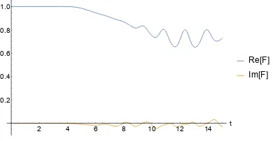
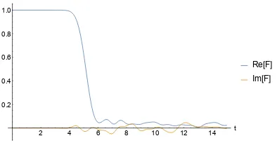
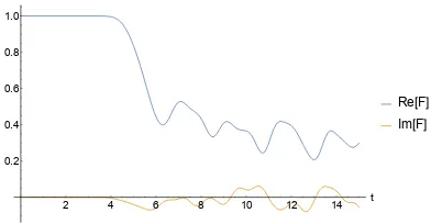
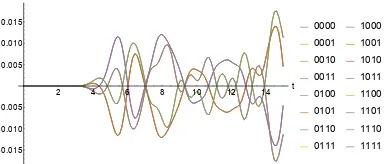
Sections 3.3 and 3.4 feature calculations of Aρ˜. First, we numerically simulate a transverse-field Ising model. A˜ρ changes significantly, we find, over time scales relevant to the OTOC. The quasiprobability’s behavior distinguishes nonintegrable

from integrable Hamiltonians. The quasiprobability’s negativity and nonreality

re-mains robust with respect to substantial quantum interference. We then calculate an average, over Brownian circuits, ofA˜ρ. Brownian circuits model chaotic dynam-ics: The system is assumed to evolve, at each time step, under random two-qubit

couplings [69–72].

A final “theory” section concerns mathematical properties and physical

interpre-tations of ˜Aρ. ˜Aρ shares some, though not all, of its properties with the KD dis-tribution. The OTOC motivates a generalization of a Bayes-type theorem obeyed

by the KD distribution [15, 73–76]. The generalization exponentially shrinks the memory required to compute weak values, in certain cases. The OTOC also

moti-vates a generalization of decompositions of quantum states ρ. This decomposition

property may help experimentalists assess how accurately they prepared the desired

initial state when measuringF(t). A time-ordered correlatorFTOC(t) analogous to F(t), we show next, depends on a quasiprobability that can reduce to a probabil-ity. The OTOC quasiprobability lies farther from classical probabilities than the

TOC quasiprobability, as the OTOC registers quantum-information scrambling that

FTOC(t) does not. Finally, we recall that the OTOC encodes three time reversals. OTOCs that encode more are moments of sums of “longer” quasiprobabilities. We conclude with theoretical and experimental opportunities.

We invite readers to familiarize themselves with the technical review, then to dip

into the sections that interest them most. The technical review is intended to

intro-duce condensed-matter, high-energy, and quantum-information readers to the KD

quasiprobability and to introduce quasiprobability and weak-measurement readers

to the OTOC. Armed with the technical review, experimentalists may wish to focus

on Sec. 3.2 and perhaps Sec. 3.3. Adherents of abstract theory may prefer Sec. 3.5.