Applying Formal Methods to Distributed Algorithms
Using Local-Global Relations
Thesis by
Jerome White
In Partial Fulfillment of the Requirements for the Degree of
Doctor of Philosophy
California Institute of Technology Pasadena, California
2011
c
2011
Contents
Acknowledgements vii
Abstract viii
1 Introduction 1
1.1 Motivation . . . 1
1.2 A Detailed Example . . . 5
1.3 Local-Global Algorithms . . . 9
1.4 Contribution and Scope . . . 20
1.5 Related Work . . . 21
1.6 Organization of the Thesis . . . 22
2 Model and Assumptions 24 2.1 System Model . . . 24
2.2 Local-Global Relations . . . 29
2.3 Correctness . . . 33
2.4 Related Work . . . 35
3 Consensus Using Monoids 38 3.1 Theorems about Monoids. . . 39
3.2 System Correctness . . . 42
3.3 Instantiations of Monoids . . . 46
4 Distributed Path Computations using Semirings 50
4.1 Central Idea . . . 51
4.2 Semirings . . . 53
4.3 System Specification . . . 54
4.4 System Correctness . . . 58
4.5 Examples . . . 60
4.6 Related Work . . . 62
5 Sorting 64 5.1 System Specification . . . 64
5.2 System Correctness . . . 68
6 Average Consensus 71 6.1 Background and Motivation . . . 71
6.2 System Specification . . . 75
6.3 System Correctness . . . 77
7 External Inputs 82 7.1 Model . . . 87
7.2 Theory . . . 88
8 Framework Extensions 91 8.1 Error Bounds with Changing Inputs. . . 91
8.2 Termination Detection . . . 92
8.3 Limits of the Local-Global Framework . . . 94
8.4 Bounds on Information Exchange . . . 97
9 Tools of Formal Methods 99 9.1 Theorem Prover . . . 100
9.2 Model Checker . . . 108
10 Conclusion and Future Work 130
10.1 Future Work . . . 130
10.2 The Applicability of Local-Global Relations . . . 132
A Auxiliary Proofs 134 A.1 Reverse Induction . . . 134
A.2 Monoids . . . 138
A.3 Mean Square Error . . . 150
A.4 Permutations . . . 153
Acknowledgements
I would first like to thank Mani, who inspired this work and allowed me the freedom to develop it. More significantly, however, there were times during the pursuit of this degree when I was unsure that I could obtain it. He always managed to convince me otherwise— something for which I am truly grateful.
This thesis would not have been possible without the help of my Infospheres labmates, especially Sayan and Concetta. Sayan introduced me to PVS, while Concetta helped to shape much of the work overall. Good scientific discoveries usually require the exploration of several bad ideas. This thesis was no exception. Concetta patiently sat through just about all of my bad ideas, time and again helping me see the error in my ways. Her insight amazes me just as much as her patience.
I would also like to thank and remember Brian, who had a significant impact on this project during its early stages. He was an incredible student and a wonderful person. I wish he could have seen the culmination of this work.
The department as a whole has been like an extended family; the faculty and staff have created a wonderful environment in which to learn as a student and to grow as a person. Maria and Mathieu, in particular, were both constant sources of encouragement, helping to make my life overall more enjoyable. Every graduate student should have people like them in their corner.
Abstract
This thesis deals with the design and analysis of distributed systems in which homogeneous, autonomous agents collaborate to achieve a common goal. The class of problems studied includes consensus algorithms in which all agents eventually come to an agreement about a specific action. The thesis proposes a framework, called local-global, for analyzing these sys-tems. A local interaction is an interaction among subsets of agents, while a global interaction is one among all agents in the system. Global interactions, in practice, are rare, yet they are the basis by which correctness of a system is measured. For example, if the problem is to compute the average of a measurement made separately by each agent, and all the agents in the system could exchange values in a single action, then the solution is straightforward: each agent gets the values of all others and computes the average independently. However, if the system consists of a large number of agents with unreliable communication, this scenario is highly unlikely. Thus, the design challenge is to ensure that sequences of local interactions lead, or converge, to the same state as a global interaction.
Chapter 1
Introduction
1.1
Motivation
1.1.1
Multi-Agent Systems Operating in Unreliable Environments
Errors in systems can have disastrous consequences. This thesis deals with designs of reliable systems in which multiple agents, operating in unreliable or hostile environments, collabo-rate to achieve a common goal. The design of such reliable systems is challenging because designers have no control over the environments in which agents operate. A system in which mobile agents communicate with each other over unreliable, wireless channels is an example of such a system. Agents communicate with others when they are in communication range of each other and they cease communication when they move out of range. The external environment determines whether and when agents can communicate. For example, enemies may jam communication among agents or the wireless environment may be noisy.
This thesis studies multi-agent systems in which designers cannot schedule interactions among agents. Designers cannot assume that an agent X will be able to interact with an agent Y some time in the future. Agents cannot control the environment which determines when agents can communicate and interact. This thesis explores undependable environments to understand the conditions under which multi-agent algorithms can operate correctly.
agent and each edge represents an interaction mechanism between a pair of agents; for example, neighboring agents in the graph can operate on shared variables in atomic actions. This thesis departs from this type of earlier work in two ways. First, agent interactions cannot be scheduled. In terms of the traditional graph representation, we consider systems in which graph edges are changed dynamically by an external mechanism over which agents have no control. Second, in cases of applications based on messages, communication may be unreliable: messages may be lost or delivered out of order.
The environment is modeled as a nondeterministic mechanism. In carrying out worst-case analysis it is helpful to treat the environment as an adversary whose intent is to thwart the agents from reaching their goals. The adversary determines which agents can interact and which messages are lost. An all-powerful adversary is uninteresting because it could prevent any agent from interacting with any other and thus stop all computations. Therefore, we consider powerful adversaries, but not all-powerful ones.
We constrain the adversarial mechanism to obey certain weak “fairness” criteria. Our goal is to understand the maximum power that the adversarial environment can have—or equivalently, the weakest fairness criteria—that still ensures that the multiagent system oper-ates correctly. For example, if a system is partitioned into two nonempty non-communicating subsets, then an agent in one subset cannot compute functions over the states of agents in the other subset. Therefore we explore algorithms in which a fairness criterion is that the system is never permanently partitioned into non-communicating subsets of agents. This thesis explores the boundaries between environments in which multi-agent computations can work and environments in which they cannot work.
illustrate the ideas by using a simple example.
Example 1 (System semantics) Each agent j has a local constant y[j] and a local vari-able x[j] of some type T. Let H be the multiset, or bag, of valuesy[j]. The goal is for each agent j to set its local variable x[j] to a common value f(H) where f is a given function that maps multisets of elements of type T to type T. For example, the local constant y[j] could be a real number and each agent j is required to set its local valuex[j] to the average of the y values. We next look at algorithms for systems with different connectivity between agents.
First consider systems that can be modeled by static graphs in which vertices represent agents and directed edges represent communication channels along which messages can be passed. To begin with consider an ideal graph in which there is a directed edge (j, k) from every agentj To every agent k. A simple algorithm is one in which each agentj broadcasts its local constanty[j] to every other agent. Thus each agent receives the local constanty[j] of every agentj, then determines the multisetH, and finally sets its local variablex[j] tof(H). An alternative algorithm is one in which agents first elect a single agent as a “leader.” All agents send their local constants to the leader. The leader determines H, computes f(H), and broadcasts f(H) to all agents. All agents then set their local variables to the result.
Next consider systems in which the environment determines which agents can interact and when. The environment picks a subset K of agents and allows communication among agents in K; agents outside K cannot communicate. Agents have no control on how K
is chosen. We can model this system by a dynamic graph in which edges are created and deleted by the environment. The environment connects all agents in a subset of agents K. That subset remains connected until either all the agents complete a step of a computation or perform the empty step in which they do not carry out an operation. The environment may then delete these edges and create edges connecting another subset of agents.
particular, if the system consists of a single agentj, then the algorithm is required to set the agent’s local variable x[j] to the given constant y[j]. Therefore, we consider algorithms of the following form: Initially each agentj sets x[j] toy[j]. When a setK of agents interacts, each agent j in K sets its local variable x[j] to f(H0) where H0 is the multiset of the local variables x[j] of agents j in K. In the case of computing the average, each agent j in a set of interacting agents sets its local value x[j] to the average of the x-values of agents in the
set. 2
This simple example illustrates some of the issues explored in the thesis:
• We study fairness constraints on agent interactions that enable algorithms to reach the desired result. We show that certain computations operate correctly even in unde-pendable environments.
• In some cases, the computation may converge to the desired result in the limit as time becomes arbitrarily large. The computation may never reach the desired result though it may get arbitrarily close. Much of the earlier work deals with formal methods to prove termination of computation. We use formal methods to prove convergence as well as termination.
• A computation can terminate only after all agents participate in the computation; if an agent never participates in a computation then that agent’s initial values cannot influence the final result. If agents do not have information about the total number of agents in the system, or some other global information, then agents cannot detect termination of a computation because the computation cannot determine whether all agents have participated in it. If agents do have information about the global state of the system, such as the numbers and id’s of agents, then they can employ more efficient algorithms, and we present such algorithms.
• Many papers deal with distributed algorithms in which the input to the algorithm is fixed. Earlier we discussed the example: compute the average over all agents j of
systems in which the input changes with time. Since inputs may change with time, the result computed by the multi-agent algorithm at each instant may be different from the result for the case where inputs are constant; we define the instantaneous error as the difference between the result computed by the algorithm and the true result. Our goal is to determine a bound on the error if such a bound exists. Consider the problem of computing the averages where the values y[j] change with time, and the agents estimate the instantaneous average of y[j] over all j; we wish to determine if the error between the estimated average and the true average is bounded.
• We use temporal logic and mechanical theorem proving systems to prove the correctness of multi-agent systems. In some cases we prove termination, and in other cases we prove convergence, and in yet other cases we prove bounds on the error.
Proving the correctness of systems of agents operating in hostile or unreliable environments is difficult. This thesis explores repeated use of a small number of formally proved algorithms to develop a large number of programs. We show how reasoning about systems using abstract algebraic concepts, such as monoids, helps in developing algorithms that are correct and implementations that are reliable. The benefit of program reuse has been demonstrated by object-oriented and compositional programming systems in which abstract components are used to create concrete programs. In these cases, development time is greatly improved by leveraging pre-built objects that are known to be correct. We consider the same idea applied to formal proofs: the cost of proving the correctness of an algorithm is amortized over multiple instances of programs that re-use that proof.
1.2
A Detailed Example
The following example presents the idea of repeated use of an algorithm and its proof. It is meant to be illustrative and is therefore described informally. A more formal treatment can be found in Chapter 3.
unique identifier that is static, and a value from a given type that is mutable. The problem is to develop a distributed algorithm by which eventually all agents reach a consensus state, where consensus is a function of the initial states of the agents. Examples of such a function include
min The state of an agent state is a number.1 The consensus state is the minimum value
in the initial states of the agents.
gcd The state of an agent is a positive integer. The consensus state is the greatest common divisor of the initial states of agents.
convex hull The state of an agent is a set of points in a two-dimensional Cartesian plane. The consensus state is the convex hull of the initial sets of points of all agents.
Agents exchange values by sending messages to a communication medium, which, in turn, determines the set of agents that will receive that message. The communication medium is faulty in the sense that messages destined for a particular set of agents can be lost, duplicated, or delivered out-of-order. Moreover, if a message is not lost, its delivery can be delayed for an arbitrary, but finite time. That is, if a messagemsent at timetis not lost, it will be delivered at some time t + ∆, where ∆ is an unknown non-negative bound. That ∆ is bounded is more important than its value: this ensures that the amount of message overtaking is finite. Initially the communication medium contains no messages and messages are not corrupted by the communication medium.2 Therefore, every message delivered to an agent was sent
by some agent.
Some papers represent distributed systems as directed graphs where the vertices are agents and the edges represent message-passing channels. In our case, the graph is dynamic in that edges are added and deleted by a mechanism outside of the programs control. Note that consensus across all the agents in the system cannot be reached if there exists a subset of agents that are permanently partitioned from the global set. Therefore, we assume that
1More generally an element of a total order.
for any non-empty proper subset of agents, messages from agents outside the subset are received by agents within the subset infinitely often.
Our goal is to write a program in an executable programming language, such as C or Java, for each agent. Consider the problem of computing the minimum of the initial values of agents. Let St(k) be the state of agent k at a point t in the computation; further, assume
that the state of an agent is an integer. The desired consensus value is x where:
x= min
k S0(k).
Agents repeatedly send a message containing their current state to subsets of agents within the system. When a messagem is received in stateS, the new state of the system S0 follows
S0 = min(S, m).
1.2.1
Correctness
In this thesis, program correctness is first demonstrated for algorithms written in a logic notation and then in a conventional programming notation, such as Java.
1.2.1.1 Algorithm Correctness
One can reason, somewhat informally, about the correctness of the program in the follow-ing way. Let M be the set of messages in the communication medium at a point in the computation. An invariant of the system is:
(x= min
k S(k)) ∧ (x≤min({M})) (1.1)
where min(M) is the minimum of all values inM. The argument for proving the invariant is that it holds initially, and that every action—sending or receiving a message, and updating state—maintains Equation 1.1.
whose state is different from x. Let D be the set of agents whose value is different from x, and let ¯D be its complement. We need to show that if D is not empty then its cardinality will decrease eventually. Our fairness assumption implies that eventually an agent inD will receive a message from an agent in ¯D. Once this occurs, the receiving agent will change its state tox and become a member of ¯D, thus reducing the variant function.
1.2.1.2 Program Correctness
To establish that a program implements a given specification, we employ a theorem prover, a model checker, and code specification languages. Algorithms are first encoded in the notation of the theorem proving system—PVS [1] in our case. Unlike “conventional” programming languages, such as C or Java, This notation uses higher-order logic, making it easier to reason about algorithm correctness. Our use of PVS can be broken into two parts: a representation phase, and a proof phase. In the representation phase, our challenge is to represent the distributed system in the logic of PVS. The proof phase consists of proving safety and progress properties of the system. It is carried out in the steps we start with, proving distributed systems that use abstract data types such as monoids. Later, we prove that concrete implementations, such as min, satisfy the axioms of the abstract types. Such proofs consist of showing algebraic properties over system operators, such as
∀a∈A: min(a, a) = a
where A is a totally ordered set. We use a theorem prover proofs that we develop by hand. We also evaluated the use of a model checker [2] within the development cycle. UsingSpin involves encoding the algorithm in Promela, which is closer to a conventional programming language than PVS. Model checkers are easier to use because they offer more automation than mechanically verifying proofs using a theorem prover.
refinement from PVS to C# are simpler than developing and proving a program in C# from scratch. For example, in this final translation step the verification requirement is to prove that an actionz= max(x, y) in Java implements the actionz = max(x, y) in PVS. Therefore, ensuring that the translation is correct is easier than deriving a correct concurrent program. For added program verification, we employ the Java Modeling Language (JML) [7], along with our own invariant assertion classes. We also provide an implementation in C#, which is similar to Java, and in Erlang [8], which demonstrates the applicability of our abstractions to other programming notations.
1.3
Local-Global Algorithms
The thesis focuses on algorithms in which the actions taken by agents in a distributed system are identical to the actions that would be taken by a single process in a non-distributed system. For example, an algorithm to compute the minimum of a set of numbers in a single process scans the numbers in the set and updates the minimum value seen so far to the smaller of its current value and the number scanned. The distributed algorithm is identical: when a subset of agents interact they compute the minimum of values in the subset.
We call these algorithms local-global because the local actions taken by subsets of agents are identical to the global actions of a single, central, process. The association between such local actions and the global state of the system is known as a local-global relation. Many distributed algorithms are not local-global: the distributed implementation is different from an implementation on a single central process. Our goal in studying local-global algorithms and relations is to understand the simplest class of distributed algorithms that are obtained by replicating a single-process centralized algorithm for subsets of agents. We identify local-global relations to generate the aforementioned algorithmic abstractions.
1.3.1
The Local-Global Concept in Algorithm Development
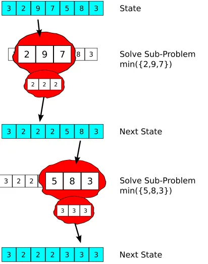
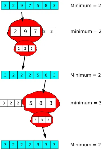
Example 2 (Minimum array value) Consider a data structure that agents may only have partial access to. That is, they can read or modify subsections of the data, but not the entire structure. In the case of computing the minimum of an array, the problem is specified in terms of the array: an agent may only be able to access a subset of elements. If the agent could operate on the entire array, then the problem is quickly solved by setting all elements of the array to the minimum value. The action carried out by the agent on the subproblem is identical to the action that an agent would carry out if it could modify the entire array: set all elements of the subarray to the minimum value of the subarray.
This is shown in Figure 1.1where the initial state is
[3,2,9,7,5,8,3]
indexed j where 0≤j <0. The first action is executed by an agent that can only read and modify elements 2 and 3 of the array. Therefore, it operates on the subarray to get a new state for the subarray as shown in the figure. The values of other parts of the data structure
remain unchanged, giving the next global state shown in the diagram. 2
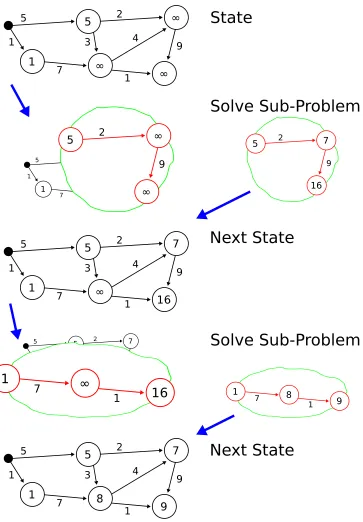
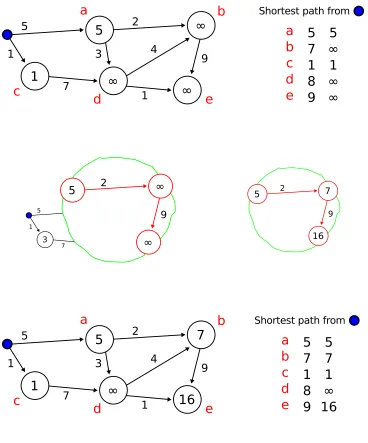
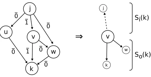
Example 3 (Shortest paths) Consider the problem of computing the lengths of the short-est paths from a vertex root to all vertices in a directed graph. If an agent can read the entire graph it solves the entire problem; that is, it computes the shortest distances to all vertices. The algorithm by which the problem is solved is irrelevant to the local-global concept.
Now consider the case where an agent can see only a part of the graph. Assume that associated with each vertex is the length of a path to that vertex; this length may not necessarily be the shortest one. An agent that can see only a part of the graph solves the shortest path problem for the subgraph that it can see. This is shown in Figure 1.2. 2
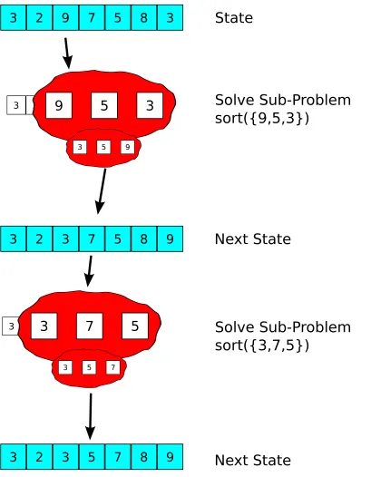
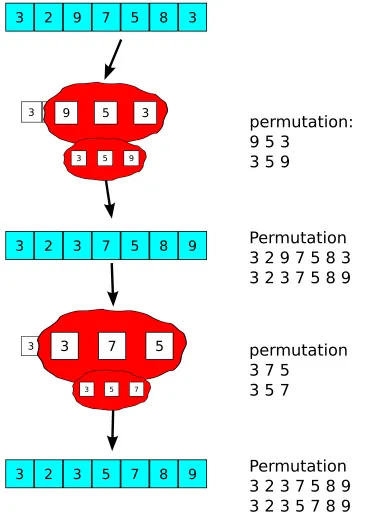
Example 4 (Sorting) Figure 1.3shows the local-global idea applied to sorting. An agent
sorts the part of the array that it can see. 2
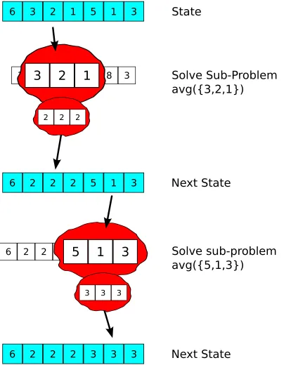
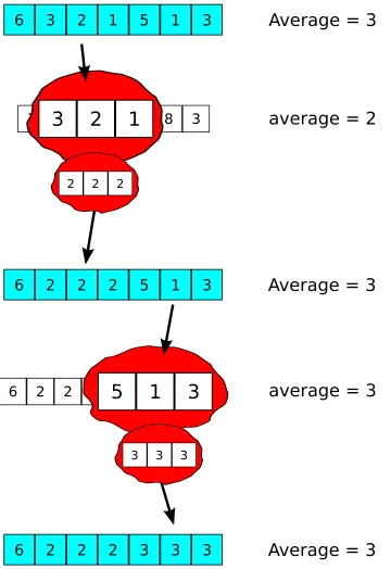
of the array. If an agent can only modify a part of the array, then it sets the values that it
can modify to the average of their values. 2
Some problems cannot be solved using the local-global approach. For example, consider the problem in which all elements of an array are to be set to its second-smallest value. Applying the local-global idea we would design an algorithm in which an agent that could operate on only a part of the array sets all the elements that it could modify to the second-smallest of their values. But this algorithm is incorrect. A local-global algorithm to compute the two smallest, or in general the k smallest, values works correctly. This thesis does not provide necessary and sufficient conditions on problem specification for the problem to be amenable to the local-global approach.
1.3.2
Local-Global Consistency in Proofs
We usually demonstrate the correctness of a centralized single-agent algorithm by providing a safety property—typically an invariant—and a progress property. We need to show that the proof for the single-agent algorithm, in which the agent has access to the entire data structure, is not violated by an algorithm in which an agent operates on only the part of the data structure that it sees.
Safety We need to prove that if a local operation on part of the data structure is safe, that it satisfies an invariant, then the local operation also keeps the global data structure safe as well.
Progress Likewise, we need to show that if a local operation on part of the data structure moves that part closer to the goal—the desired end state for that part—then that local operation also moves the global data structure closer to the global goal. Further, we need to show that a local operation that moves a local part of the data structure will be executed eventually; we do so using specialized fairness arguments.
progress properties of the entire data structure. Then we use this generic approach repeatedly for all the problems considered in the thesis.
1.4
Contribution and Scope
1.4.1
Reducing the Cost of Verification
Although formal methods are recognized as being beneficial in preventing software errors, that recognition comes largely from within the research community. Part of this disparity stems from the fact that formal methods can be difficult for non-experts to use. Formal proofs that are mechanically verified provide high confidence in a programs correctness, but require an understanding of predicate calculus and an expertise in a problems domain. Model checking works by systematically checking program paths and analyzing program state in search of various error conditions. This approach can provide detailed insight into why a particular error might occur, but might not find such errors when a programs state space is large [9]. Using specification languages can be difficult for large programs. Targeting where specifications should be placed and the proper level of discourse they should display can be difficult for developers [10].
1.4.2
Limits to Local-Global Computations
Systems in which agents can orchestrate interactions perfectly will have better performance than systems in which agent interactions are determined by an external mechanism. Likewise, systems in which agents can send messages to any other agent without message loss will have better performance than systems in which messages get lost. An issue we explore is how much performance is lost by multi-agent systems operating in uncertain and hostile environments compared to performance in ideal environments. This analysis evaluates the total time, the total number of messages, and the total volume of information exchanged, in the ideal environment and a hostile environment. If we only make fairness assumptions about agent interactions, then the ratio between the best and worst cases can be unbounded. Therefore, we also carry out analysis with tighter constraints on mechanisms for agent interaction.
We study algorithms for termination detection for systems in which agent interactions are determined by external agencies. Many of the termination detection algorithms in the literature assume that agent interactions are specified by static graphs in which vertices represent agents and edges represent shared variables or message-passing channels. The termination-detection algorithms studied here have to operate in an environment in which algorithm designers do not know which interactions can occur and when.
1.5
Related Work
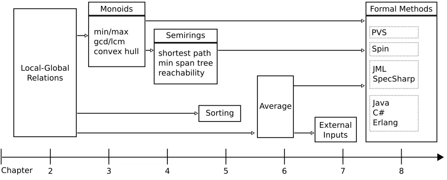
Figure 1.9: Thesis outline. Each box represents a chapter—its main points listed therein.
While we share in this goal, we are also trying to build a library of reusable proofs.
Simplifying formal methods for program development has been studied by M¨oller [14]. He approaches the problem from a very theoretical level, first defining, then applying, an algebra of formal languages that is reusable across problem domains. As is the case in our formalization, he identifies key properties necessary for concrete operators to posses— associativity and commutativity, for example. He applies his formalization to sorting and graph problems, which our formalization maps to as well (Sections 4 and 5, respectively).
1.6
Organization of the Thesis
Chapter 2
Model and Assumptions
The first section of this chapter reviews widely-used models for distributed systems. The material is presented here for completeness. Section 2.2 introduces the basic idea of local-global relations and algorithms that were introduced in Chapter 1.
2.1
System Model
Next, we present a brief review of labeled transition systems.
Definition 1 (Labeled Transition System) A labeled transition system is an ordered quadruple, (S,Λ,L,_), where: S is a set of states, Λ ⊆ S a set of start states, L a set of labels, and_⊆ S × L × S a ternary relation defining transitions between states. 2
The set of labels are associated with “actions” of agents in a distributed system; for example, an action may be to send a message containing the current state of the agent. A state transition is represented by
S _l S0
where S is the state before the transition, S0 is the state after the transition, and l is the label or the action that caused the transition. The execution of an action l when the system is in state S may result in one of many possible next states. For example, let S, S0 and S00
Figure 2.1: A graphical representation of a labeled transitions system. Darkened agents denote possible start states.
computation of averages: the action modifies the values of real variables in a set of agents so that the average of the values remains unchanged and the sum of squares is reduced by
at least p percent. This action does not specify the precise amount by which the sum of squares should be reduced; this action can take the system from a given state to different next states depending on how much the sum of squares is reduced.
A labeled transition system with a finite number of states can be represented by a labeled directed graph in which the vertices represent states and the labeled directed edges represent transitions between states. There may be many outgoing edges with the same label from the same vertex. In some models, actions are deterministic—for each label and each vertex there is at most one outgoing edge with that label. In some models, such as unity [15], actions are deterministic and any action can be executed in any state (though the action may be askip which does not change the state); in the corresponding graph model, for each label and each vertex, there is exactly one outgoing edge with that label.
An execution of a transition system is a sequence of state transitions, starting from an initial state, where the end-state of each transition is the start-state of the next transition.
n
where i ∈ N0, l ∈ L, and S, S0 ∈ S. In terms of the graph, an execution is a path in the graph starting at an initial state represented by a root vertex (Figure 2.1). It is sometimes convenient to denote the execution in a sequential, rather than set-builder, notation:
S0
l0 _S1
l1 _. . .
li _Si
li+1 _ . . . ,
where S0 ∈ Λ and ∀i ∈ N0: (Si, li, Si+1) ∈_. We make the assumption made in unity that for each label l and each state S there is at least one transition from S, which may be a “skip” from S back to itself. This assumption simplifies the model when we discuss fairness. Because of this assumption, for each stateS there exists an infinite execution from
S, though that execution may remain in the same state forever.
2.1.1
Distributed Systems
A distributed system is a fixed finite set A of agents and a labeled transition system that has the following properties. Let N be the number of agents. Associated with each agent v
is a set Tv of agent states and a subset of these states called the initial states of v. In most
of the applications studied in this thesis all agents have the same sets of agent states; so, we drop the subscript v and refer to the set of agent states as T. The properties we require of a distributed system are:
1. A state in the transition system is anN-tuple of agent states, whereN ∈N0. We refer to a state of the transition system as a global state or system state, and to the state of an agent as a local state or an agent state.
2. Each transition leaves the states of some subset of agents unchanged and may change the states of agents that are not in the set. We use the label l ∈ L for any transition that may change the states of a set l of agents while leaving the states of agents not inl unchanged.
Channels and message communication media are modeled as agents. For example, the mes-sage communication medium described in the previous chapter is modeled as a set of mesmes-sages in transit. The state transition corresponding to delivering a message from this set to an agentv may change the state of the communication medium and agentv but leave the states of all other agents unchanged.
We use S(k) to denote the state of an agentk when the global state is S. A global state is represented either as an N-tuple or as a set {(k, S(k)) | k ∈ A ∧S ∈ S} of pairs. We denote the restriction of S to a subset of agents K ⊆ A byS|K.
S|K = {(k, S(k)) | k∈K}.
2.1.2
Fair Executions
An execution in which agents in one subsetK never interact with agents in the complemen-tary set cannot reach a global consensus or reach other global goals because agents inKnever have information about agents that are not in K. Therefore we restrict infinite executions to have certain fairness properties.
Many models have fairness criteria that all actions are executed infinitely often in an infinite execution. Thus, in these models, for each pointtin an infinite fair computation, for each action l, there is a later point t0 at which action l is executed. Most of the programs discussed in this thesis rely on a weaker model: We only require that the set of agents are not permanently partitioned into subsetsK and ¯K where no action is executed that includes agents in both K and ¯K (see Figure 2.2). The fairness criterion in this case is that for every non-empty proper subset K of agents: actions that are executed jointly by agents in bothK
and ¯K are executed infinitely often in an infinite fair execution.
Figure 2.2: In afair execution, agents will never be permanently partitioned. During an exe-cution, agents communicate within groups;K andJ above, for example. However, infinitely often, eventually agents will communicate across these partitions, such as the darkened agents above.
computation there is a later point t0 at which one of these actions is executed in an infinite fair computation. Let FK be the set of actions that include an agent from K and an agent
from ¯K; then the fairness requirement is that each point t in an infinite fair computation there is a later point t0 at which one of the actions in FK is executed.
A different set of agents, say J = {0,2}, also has a fairness requirement to ensure that agents inJ can interact with agents outsideJ. This reasoning gives us the following fairness requirement:
Definition 2 (Fair Execution) A fairness condition F for a set of transitions is a finite collection{Fi}
n
i=1, where eachFi is a non-empty subset ofL. An infinite sequence of actions
l1, l2, . . . is fair if and only if
∀F ∈ F, ∀n ∈N0, ∃m∈N0: m > n ∧ lm ∈F. 2
Definition 2 requires that infinitely often a spanning tree of the communication graph is formed, regardless of which spanning tree that is. This specification is a weaker model of fairness than traditional weak fairness assumptions [16]. By reducing all FK ∈ F to
Figure 2.3: A local-global relation. Consider the transition S _K S0, denoted above. The “local” minimum value—the minimum value of the subset of agentsK—inS is equal to the local minimum value in S0. Likewise, when the minimum value over the global state of the system is calculated, that value is also equal in both S and S0 as well.
2.2
Local-Global Relations
As we discussed in the previous chapter, we study a class of algorithms in which the compu-tational steps taken by any subset of agents that participate in an action are the same as the steps taken ifall the agents in the system participate in an action. In other words, the steps taken by any subset of agents in an action are the same as those taken by a single, central process with access to all the data. We used the simple example of computing the minimum of a set of values: if all the agents in a system can participate in an atomic interaction then each agent sets its value to the minimum of the values of all the agents. Likewise, when all the agents in any subsystem participate in an interaction, each agent sets its value to the minimum of the values of all agents in the subset.
Many problems cannot be solved by algorithms in this manner; that is, in which local actions of agents in a distributed system are identical to the actions of a single central process. Some interesting problems, however, can be solved in this way. Here we explore some properties of problems that allow for the development of such algorithms.
minimum. Let the global state of the system, with agents indexed 0, 1, 2, be
{(0,5),(1,7),(2,4)},
where a pair (k, S(k)) identifies an agent k and its state S(k). When any set K of agents participates in an interaction, each agent inK sets its value to the minimum of the values of all agents in K. For example, if agents 0 and 1 participate in an interaction then the global state after the interaction is
{(0,5),(1,5),(2,4)}.
The minimum of the values of the agents in K—the value 5—is not changed by the action. Moreover, the minimum of the values of all the agents in the system—the value 4—is not changed by the action either. This property is an example of a conservation law: if a property is conserved locally then it is also conserved globally. We capture this notion by the following definition of a local-global relation between states. The form of the conservation law for the minimum example is:
(min({S(k) | k ∈K}) = min({S0(k)| k ∈K})) ^ (∀j /∈K: S(j) =S0(j)) =⇒
min({S(k)| k ∈ A}) = min({S0(k) | k∈ A}).
We generalize this idea to local-global relations between states of sets of agents.
Definition 3 (Local-Global Relation) Let be a transitive binary relation between system-states. A local-global relation follows
∀K ⊆ A, j /∈K: S|KS0|K
^
S(j) = S0(j) =⇒ S|AS0|A.
2
state of the system be
{(0,5),(1,7),(2,4)}.
The second smallest value in the system is 4, which the agents should agree upon at some point during the execution. However, consider the case where agents 1 and 2 interact; the global state of the system is updated as follows
{(0,5),(1,7),(2,7)}.
In this post-interaction state, the correct consensus value is lost and the local-global relation is violated:
min2({7,4}) = min2({7,7});min2({5,7,4}) = min2({5,7,7}).
The equality relation holds in the antecedent, 7 = 7, but not in the consequent, where 56= 7.
Theorem 1 (Reduced Local-Global Relation) Let be a transitive binary relation be-tween system-states. If
∀K ⊆ A, j /∈K:
S|KS0|K
^
S(j) =S0(j)
=⇒ S|K∪ {j}S0|K∪ {j}
holds where K is not empty, then is a local-global relation. 2
Proof The proof is by reverse induction onK: We first prove the theorem for the full set of agents. We then assume its correctness for a general set of agents, and use this assumption to show correctness for a smaller set. This scheme is formally outlined in Section A.1.
Base Case Let K be the full set of agentsA:
∀S, S0 ∈ A: S|AS0|A∧ ∀j /∈ A: S(j) =S0(j) =⇒ S|AS0|A.
Inductive Step For all S, S0 ∈ A,
S|K∪ {k}S0|K∪ {k}∧ ∀j /∈(K ∪ {k}) : S(j) =S0(j) =⇒ S|AS0|A
^
(2.1)
S|K S0|K∧ ∀j /∈K: S(j) = S0(j) (2.2)
=⇒
S|AS0|A, (2.3)
where k /∈ K. Equation 2.3 follows directly from the consequent in Equation 2.1; however, to use that consequent we must discharge its antecedent—a two-step process because of the conjunction. Assuming Equation 2.2,
1. S|K S0|K =⇒ S|K∪ {k}S0|K∪ {k}, which follows by assumption.
2. ∀j /∈ K: S(j) = S0(j) =⇒ ∀j /∈ (K ∪ {k}) : S(j) = S0(j), which holds since
(A \(K ∪ {k}))((A \K).
The local-global theory is very general: it talks about neither the nature of the commu-nication nor the computation, that takes place between agents. Thus, assuming that the computation is done locally, the local group size determines the amount of time required to solve a given problem. In the worst case, a set of agents performs only pairwise calculations; while the best case is one in which all agents form a single group after system initialization. Another method for use the local-global framework is for agents to only exchange infor-mation about their initial state, and perform the computation “offline” once they have a complete understanding of the global state. In theory, such a methodology is acceptable as long as the implicit assumptions about our framework are obeyed:
1. commutativity of the operation is preserved. If agents are to perform the computation over the global state of the system, the order in which they process individual agent values should not matter;
in this thesis is required;
3. and, a protocol for determining when all states of all agents have been exchanged must be put in place. Without such knowledge, agents will never perform the underlying computation. Although the local-global framework as we have presented it does not mention termination, as we will see inSection 2.3.2, the system still makes incremental progress during execution.
In practice, performing delayed global computation is not always practical; for instance, when a large number of agents are in the system. In this case, an implementation may fail or perform poorly due to memory and computational constraints. By performing solving the problem locally, our framework deals with such issues in-place.
2.3
Correctness
2.3.1
Invariants
An actionl is said to satisfy a local-global relation if and only if any transition from state
S to any stateS0 due to execution of action l satisfiesS|KS0|K. Formally,
∀l ∈ L, K ⊆ A: K =l ∧ S _l S0 =⇒ S|K S0|K. (2.4)
Theorem 2 (Maintaining Local-Global Relations) If all actions of a transition system satisfy a local-global relation, then the system has the following invariant:
Invariant: S0|ASt|A. 2
Proof of Theorem 2 follows from transitivity on .
type. Consider defined as
∀K ⊆ A: S|KS0|K ≡ f(S|K) =f(S0|K).
If all actions of a transition system satisfy , then an invariant of the system is
Invariant: f(S0) =f(S). 2
Corollary 2 (Non-increasing) Letf be a monotone function from states of sets of agents to some totally ordered set. Consider defined as
∀K ⊆ A: S|K S0|K ≡ f(S|K)≥f(S0|K).
If all actions of a transition system satisfy , then an invariant of the system is
Invariant: f(S0)≥f(S). 2
2.3.2
Progress
Letd be a function from states to a partially ordered set P that has a unique lower bound,
G be an invariant of the system, and Q be a predicate on global states of the system. We are interested in sufficient conditions for proving that eventually Q holds. This section lays the ground work for that proof by showing that there are only two possible outcomes for a given fair execution: either Q holds, or d strictly decreases. The following theorem is taken from the literature [17]; we state it here without proof.
Theorem 3 (System Progress) [17] If the following hold D1. ∀k ∈ A, K ⊆ A:G(S)∧S _K S0 =⇒ d(S)≥d(S0)
D2. ∃FK ∈ F,∀K ∈FK: G(S)∧ ¬Q(S)∧S K
_S
then, for all executions, either
E1. for all p ∈ P, if d(S) = p at any point in an execution, then there is an infinite suffix of the execution where d(S)< p for all states in the suffix:
∀p∈P: 2(d(S) =p =⇒ 32d(S)< p),
or
E2. every execution has a suffix where Q holds at every point in the suffix:
32Q(S0).
2
Theorem 4 (Local-Global System Progress) If the following hold H1. ∀K ⊆ A:G(S)∧S _K S0 =⇒ d(S|K)≥d(S0|K)
H2. ∃F ∈ F,∀K ∈F: G(S)∧ ¬Q(S)∧S _K S0 =⇒ d(S|K)> d(S0|K), and
H3. d is a local-global relation with respect to > and ≥,
then, for all complete executions, either E1 or E2 holds. 2
Proof Since d is a local-global relation, the following implications hold by definition:
d(S|K)≥d(S0|K) =⇒ d(S)≥d(S0)
^
d(S|K)> d(S0|K) =⇒ d(S)> d(S0).
2.4
Related Work
have considered such dynamics when studying living systems, such as molecular develop-ment [18, 19] and swarm intelligence [20, 21]. Understanding the nature of such biological systems well enough to mimic their behavior in computing systems is a focus of the amor-phous computing [22, 23] and self-assembly communities. Although they have different ap-proaches, both areas study how autonomous processes can build structures or create patterns. Instead of having a blueprint for the final product, these processes possess only instructions on how to interact. The challenge for scientists is to formally describe these instructions. To this end, graph grammars have been considered [24,25] and new languages developed— growing point language (GPL) [26], origami shape language (OSL) [27], and Proto [28], for example. These efforts take more of an engineering stance toward the process, concentrating on the primitives for solving specific problems, rather than on understanding the advantages and limitations of local interactions.
Recent work by Daniel Yamins has been an attempt to bridge this gap. He too is explicitly interested in formally explaining global structures built from local rules. To characterize local interactions, Yamins defines a function intended to be run over some set of agents, and a means of composing that function—similar to our transition semantics. In early work, his primary applications is to the one-dimensional equigrouping problem [29, 30]. Later work applies this model to other formation problems, and offers deeper insight into its implications [31, 32, 33]. While Yamins is also interested identifying local interactions in much the same way we do, he does not consider it for proof reuse. Interesting future work would be for us to apply our model to his examples.
generic solution. Indeed, LGI could enforce that agent interactions fit our local-global model. Moreover, we make the assumption that all agents within the system are homogeneous with respect to their state update—LGI could be utilized to verify this assumption at run time.
Locally stable predicates are another means of identifying global system properties based on local, per-agent, information. A predicate is defined to be locally stable if it holds eventually-always for a subset of agents [40, 41]. Work in this area has focused mostly on termination and deadlock detection: algorithms analyze subsets of global snapshots to make a decision about the global state of the system. The analysis can be reduced to Boolean algebra, which is an example of a local-global relation as we have defined them. Thus, locally stable predicates can be described using our framework.
Chapter 3
Consensus Using Monoids
Given a set of agents, the goal of a distributed consensus algorithm is for all agents to come to a consensus value. In this chapter we consider distributed consensus problems specified as follows. LetS0 be the initial state of the system with S0(k) the initial value of the agent indexed k. Desired consensus states are specified as a function f from global states S to local states, T:
f: S → T.
In the case of the example of computing the minimum, the desired consensus agent state is the minimum of the values of the initial agent states.
A consensus global stateS? is one in which all agentsk0, k1, . . . , kn−1 are in the consensus agent state f(S0),
S? ={(k0, f(S0)),(k1, f(S0)), . . . ,(kn−1, f(S0))}.
In this chapter we consider problems that require the system to enter, and remain thereafter, in the consensus stateS?. That is, in any infinite fair computation, if S
0 is the initial state then eventually the computation enters a point after which the state is always S?; in the
notation of temporal logic:
S0 =⇒ 32S?.
state in the limit.
This chapter restricts attention to functions f which is a folding [43, 44] of the initial values of the agents with an operator⊕; for example, if the agents are indexedk= 0, . . . , n− 1, then
f(S) = S(0)⊕S(1)⊕. . .⊕S(n−1). (3.1)
In the case of computing the minimum, ⊕ is the min operator. We restrict attention to operators ⊕ that are associative and commutative and have an identity element. Thus, the agent states and the operator form a commutative monoid [45]. For completeness we review the definition of monoids.
Definition 4 (Monoid) A monoid consists of the pair,hT,⊕i, whereT is a set of elements, and ⊕ is a binary operation on those elements. The operator ⊕ is associative and closed over T, and there exists an identity element in T:
∃a∈T,∀b ∈T:a⊕b=b⊕a=b.
2
A monoid is said to be commutative if ⊕ is also commutative with respect to T. For the remainder of this chapter, we restrict attention to commutative monoids where the operator ⊕ is idempotent:
∀a∈T: a⊕a=a.
We first give lemmas without assuming idempotence, and later give lemmas that assume it.
3.1
Theorems about Monoids
Figure 3.1: An example of monoid composition. Consider a system transition, S _K S0, where the K is the set of blue agents. The monoid applied during a transition is hN0,mini, with an identity element of ∞. The sequence of min applications (pictured between states) is an example of how an agent within K uses composition (Definition 6) to update its state.
Definition 5 (Monotonic) Let≥be an ordering relation over elements in T, where ∀a∈ T : a≥a. A binary operation, ⊕: T → T, is monotonic when
∀a, b, c∈ T : a≥b =⇒ a⊕c≥b⊕c.
2
Let⊕ be the min operator. An example of Definition 5 follows
a ≥b =⇒ min(a, c)≥min(b, c).
Definition 6 (Monoid Composition) LethT,⊕ibe a commutative monoid with identity element ¯0, where ⊕ is also monotonic. Recall that T is the type of the agent state. Let
K ⊆ A. The L
operation is defined to be the following composition function over the monoid:
M
k∈K
S(k) =
¯
0 if K =∅,
∀j ∈K: S(j)⊕ M
i∈K\{j}
S(i) otherwise. (3.2)
2
Lemma 1
M
k∈K∪ {j}
S(k) =M
k∈K
S(k)⊕
¯
0 if j ∈K,
S(j) otherwise.
2
Proof There are two cases to consider: where j is a member of K, and where it is not. In the former, the lemma holds since ¯0 is the identity element:
j ∈K =⇒ M
K∪ {j}
S =M
K
S⊕¯0
=⇒ M
K
S=M
K
S⊕¯0
=⇒ M
K
S=M
K
S.
The second case holds by definition
k∈K ∪ {k} =⇒ M
K∪ {k}
S =S(k)⊕ M
K∪ {k}\{k}
S ^ (3.3)
k /∈K ∪ {k} =⇒
M
K∪ {k}
S=S(k)⊕M
K
S, (3.4)
where 3.3 is the definition of fold with K =K ∪ {k}. We can safely assume the antecedent in 3.3, since k ∈ K ∪ {k} is a tautology. Further, K ∪ {k} \ {k} = K. Such rewrites
3.2
System Correctness
Theorem 5 (Monoid Composition is Local-Global) Let ≥ be a transitive relation on elements in T.
M
k∈K
S(k)≥M
k∈K
S0(k) ∧ S|{j} =S0|{j} =⇒
M
k∈K∪ {j}
S(k)≥ M
k∈K∪ {j}
S0(k),
where j /∈K. Note, that when the relation is equality:
M
k∈K
S(k) = M
k∈K
S0(k) ∧ S|{j} =S0|{j} =⇒
M
k∈K∪ {j}
S(k) = M
k∈K∪ {j}
S0(k).
2
Proof Follows from Lemma 1 and assumed monotonicity of ⊕ with respect to≥.
Definition 7 (Consensus Transition) A transition, S_K S0 is≥-preserving if and only if
S _K S0 =⇒ M
k∈K
S(k)≥M
k∈K
S0(k).
2
Corollary 3 (Local-Global Invariant Property) If all state transitions preserve≥, then
Invariant: M
k∈A
S0(k)≥
M
k∈A
S(k).
If all state transitions preserve =, then
Invariant: M
k∈A
S0(k) =
M
k∈A
S(k).
2
Proof Follows from Theorem 5and Theorem 2.
properties outlined in its definition (Definition 4). Others have used recursive operators to simplify inductive proofs [43,44] for sequential algorithms but not for distributed systems.
Progress
We use Theorem 3 to prove progress. Recall that the theorem requires an invariant of the systemG, along with a predicateQand distance functiondon the state space. We introduce a mapping g: S × A →2A to facilitate the definition of these elements. An invariant of the system is that for all agents k the state S(k) is the ⊕ operator applied to all elements of some setK of agents; let g(S, k) be the largest such set. Initially,
∀k ∈ A: g(S0, k) = {k}.
When agents interact, the mapping is updated:
S _K S0 =⇒ g(S0, k) =
g(S, k) ∪ S
j∈Kg(S, j) if k ∈K,
g(S, k) otherwise.
Definition 8 (Progress Variables) The predicates G and Q on the state space of the system are
G(S)≡ ∀k ∈ A: S(k) = M
j∈g(S,k)
S0(j)
Q(S)≡ ∀k ∈ A: g(S, k) = A.
The variant, or Lyapunov, function d is
d(S) = n−X
k∈A
|g(S, k)|
Figure 3.2: Evolution of the variant function g during an execution. Darkened nodes repre-sent the range of g when applied to agent b in a given state; agent interactions are under-scored. For example, in state S2, agents cand d interact, while g(S2(b) ={a, b}. Note that the transition from S3 to S4 completes the communication graph for agent b even though b has only participated in two transitions.
The predicate G holds in state S if the state of each agent is equal to ⊕-composition of the start state, restricted to agents in g; see Figure 3.2 for a visual interpretation. The predicate Q holds in S if the set defined by g holds all agents in the system. Finally, the distance function d is a measure of partitioned agents in a given state.
Lemma 2 The predicate G is an invariant of the system. 2
Proof The proof is by induction onS:
Base Case Consider the start state, G(S0):
S0(k) =
M
j∈g(S0,k)
S0(j)
= M
j∈{k}
S0(j)
Inductive Step Assume G(St) and St K
_St+1. Let J =
S
j∈Kg(S, j). It follows that,
St+1(k) =
M
j∈g(St+1,k)
S0(j)
= M
j∈g(St,k)∪J
S0(j).
Because J ⊆ A the equation holds from properties on the monoid.
Theorem 6
∀k ∈ A, K ⊆ A: G(S)∧S _K S0 =⇒ d(S)≥d(S0)
2
Proof From the definition of actions,
S _K S0 =⇒ g(S, k)⊆g(S0, k)
=⇒ |A \g(S, k)| ≥ |A \g(S0, k)| =⇒ d(Sk)≥d(Sk0)
=⇒ d(S)≥d(S0).
Theorem 7
∃FK ∈ F,∀K ∈FK:G(S)∧ ¬Q(S)∧S K
_S 0
=⇒ d(S)> d(S0)
2
Proof By definition,
¬Q(S) =⇒ ∃k∈ A: g(S, k)6=A.
Using this to choose our instance ofFK ∈ F:
A similar argument to the proof of Theorem 6 follows1
S (_j,k)S0 =⇒ g(S, k)(g(S0, k)
=⇒ d(S)> d(S0).
3.3
Instantiations of Monoids
Thus far, our theory has been presented in terms of the generic operator⊕. The advantage of our abstract theory is that when applying it to concrete examples, proofs of system correctness are reduced to algebraic proofs on monoid instances.
Example 6 (Min/Max) We briefly discussed a system built around the minimum operator earlier in this section. To review, the objective of the system is for each agent to contain the lowest value in the system. The dual of this algorithm is for agents to end up with the maximum value. We consider both cases.
Proof Obligation
For a total order Z, hZ,mini, with identity element +∞, forms a commutative monoid that is idempotent. The local-global relation is equality.
• ∀a∈Z: min(a,+∞) = a
• ∀a, b∈Z: min(a, b)∈Z
• ∀a, b∈Z: min(a, b) = min(b, a)
• ∀a, b, c∈Z: min(a,min(b, c)) = min(min(a, b), c)
Definition 9 (Min and Max) The minimum and maximum values over a set of natural numbers S is defined:
min : i, j →if i < j then i else j
max : i, j →if i < j then j else i. 2
When calculating the minimum consensus, the monoid is hN0,mini; when finding the maxi-mum consensus, the monoid is hN0,maxi. Proofs that these structures fit a monoid can be found inSection A.2.2. In either case, the relations≥, in the case of min, and ≤, in the case of max, could be substituted for equality. We consider this relation in Chapter 4. 2
Example 7 (GCD/LCM) The objective of the system is to agree on the greatest com-mon divisor (gcd) or least comcom-mon multiple (lcm) of the agents. Before discussing their applicability to monoids and local-global relations, we provide a definition.
Proof Obligation
For a total order N1, hN1,lcmi, with identity element 1, forms a commutative monoid that is idempotent.
• ∀a∈N1: lcm(a,1) =a • ∀a, b∈N1: lcm(a, b)∈N1 • ∀a, b∈N1: lcm(a, b) = lcm(b, a)
• ∀a, b, c∈N1: lcm(a,lcm(b, c)) = lcm(lcm(a, b), c)
A similar set of obligations exist for gcd. Definition 10 (Divisibility)
divides : i, j → ∃x: j =i×x
Definition 11 (LCM and GCD)
gcd : i, j →max{k | divides(k, i)∧divides(k, j)}
lcm : i, j →min{k | divides(i, k)∧divides(j, k)}
where i,j, and k are all positive natural numbers.2 2
For lcm consensus, the proper monoid ishN1,lcmi; for gcd the monoid is hN0,gcdi. In both cases, the local-global relation is equality. Formal proofs can be found in Section A.2.2. 2
Example 8 (Convex Hull) The convex hull of a given set of points is the minimum set of points in which all other points are contained. Agent state consists of a set of coordinates on a plane. They maintain their current position, as well as set of points that represent the convex hull. Denote byCh: P →P the convex hull of a set of points that produces another
set of points. When agents interact, they exchange coordinate information and apply Ch to
update their current knowledge about the convex hull. The objective of the system is for all agents to agree on what the convex hull is. The monoid that describes this algorithm is hR,Chi, where equality is the local-global relation.
Proof Obligation
For a total orderT, hT,Chi, with identity element ∅, forms a commutative monoid
that is idempotent.
• ∀a∈ T : Ch(a,) = a
• ∀a, b∈ T :Ch(a, b)∈ T
• ∀a, b∈ T :Ch(a, b) = Ch(b, a)
• ∀a, b, c∈ T : Ch(a,Ch(b, c)) = Ch(Ch(a, b), c)
Proofs of such can be found in Section A.2.2. 2
3.4
Message Passing
Consider a lossy message-passing medium discussed earlier where messages may be lost, duplicated an delivered out of order. The fairness requirement is that for any set K of agents, a message from some agents in ¯K, the complement of K, reaches some agent in K
infinitely often.
We treat the communication medium as an agent with a different state space. Let M be the state of the communication medium; then M is a bag, or multiset, of messages in transit. Proof of the invariant
Invariant: M
k∈A
S0(k) =
M
k∈A
S(k)
!
^ M
k∈A
S0(k) =
M
k∈A
S(k)⊕ M
m∈M
S(m)
!
Chapter 4
Distributed Path Computations using
Semirings
Consider a distributed computation of shortest paths in a directed graph in which there is an agent at each vertex. An agent’s state includes information about the weights of edges incident on that agent’s vertex. We assume that the graph is strongly connected and that there are no negative-weight cycles in the graph. All agents compute the length of the shortest path to them from a special agent called the “source.” The problem of computing the path from the source to all agents, is called the single-source problem; it can be extended in a straightforward way to the all-points shortest path problem in which all agents compute the lengths of the shortest paths to all other agents.
4.1
Central Idea
We describe the idea starting with the shortest path algorithm. Assume that vertices are indexed k = 0,1, . . . , N −1, for N >0. Let W[j, k] be the weight of the edge from vertex j
to vertex k if the directed edge (j, k) exists. The problem is to compute the shortest path from a vertex, called the “source,” to all other vertices. Let us assume that the source is vertex 0. If there is no path from the source to a vertex k, then the length of the shortest path to vertex k is infinity. Let D[k] be the length of the shortest path from vertex 0 to vertex k. Since no cycles of negative length exist,D[0] = 0.
Each vertex is associated with an agent. The state of agent k includes the values of the edge weightsW[j, k] for allj, and the set of vertices to which there there is an outgoing edge fromk.
A distributed version of the well-known sequential algorithm is as follows. Associated with each agent k is a local variable w[k] which eventually becomes D[k], the shortest distance from the source to vertexk. Also, each agent k has a local variableparent[k] which eventually becomes the prefinal vertex on the shortest path from the source to k; in other words a shortest path from the source to vertex k goes from the source to vertex parent[k] and then traverses the edge from parent[k] to k.
Initial Condition The initial condition of the algorithm is:
w[source] = 0 ∀k6=source: w[k] =∞
∀k: parent[k] =source.
Rules of the Algorithm The algorithm is given by a set of rules, with one rule for each ordered pair, (j, k):
if w[k]> w[j] +W[j, k]then
w[k]←w[j] +W[j, k]
end if.
We refer to the inequality condition as the triangle property.
Rules are selected non-deterministically. The fairness criterion is that every rule is executed infinitely often.
Invariant An invariant of the algorithm is that for all k, w[k] is either infinity or it is the length ofa path from the source to k that goes from the source toparent[k] and then along the edge from parent[k] to k. We give a proof of this invariant for the general case of semirings later.
Progress We prove progress using a variant function in the usual way: we show that (i) for all actions, execution of the action does not increase the value of the variant function, and (ii) if the desired predicate is not reached then there exists an action that is executed infinitely often that decreases the variant function.
A variant function for this problem is as follows. For each vertex k, rank order all the cycle-free paths from the source to a vertexk in increasing order of distance and index the paths with 0,1,2, . . . in the sequence, with the shortest path having index 0 and a fictitious path of infinite length having the largest index. There are a bounded number of such cycle-free paths in a finite graph. In each state, the value of w[k] corresponds to a path from the source to vertex k and therefore corresponds to an index in this sequence; let us call this index r[k]. The variant function f is the sum of the indexes of all agents.
f =X
k∈A
r[k]
We first show that the variant function does not increase in value as computation proceeds. For any agent k, the execution of any action decreases w[k] or leaves it unchanged; therefore the execution of any action does not increase r[k].
variant function. To do so we show that if the desired predicate does not hold then there exists some edge (j, k) such that the triangle property does not hold:
w[k]6> w[j] +W[j, k].
Discussion Consider another path problem, such as computing reachability of vertexes from a source vertex. We could carry out a similar argument as for the shortest path problem. The use of abstract algebra reduces the amount of work required to prove the correctness of distributed algorithms for similar sorts of problems.
The arguments for correctness of the algorithm given above cannot be verified by a mechanical proof checker. This is because the arguments use natural, English-like, language to talk about concepts in graphs. A great deal of effort is required to develop proofs that can be verified by a program; this effort is amortized over several problems by presenting and proving an algorithm using data structures from abstract algebra.
4.2
Semirings
We extend the monoid introduced in Section 3.1 and applied in Chapter 3, to semirings.
Definition 12 (Semiring) A semiring consists of the quintuple, hT,⊕,⊗,¯0,¯1i, such that • hT,⊕i is a commutative monoid with identity element ¯0,
• hT,⊗i is a monoid with identity element ¯1,
• ⊗ distributes over⊕, and
• ¯0 is an annihilator1 when used with ⊗. 2
• ⊕ is idempotent, and
• ¯1 is an annihilator for ⊕. 2
Theorem 8 (Semiring Partial Order) Given an idempotent semiring, defines a par-tial order over T such that ∀a, b∈ T :ba ⇐⇒ a⊕b =a. 2
Proof Reflexivity follows directly from the definition and idempotence. Anti-symmetry:
a =a⊕b = (a⊕b)⊕b = (b⊕a)⊕b =b⊕b = b. Transitivity: a = a⊕b = a⊕(b⊕c) =
(a⊕b)⊕c=a⊕c.
Theorem 9 (Bounded Semiring) Given an idempotent semiring,
∀t∈ T : ¯0t¯1.
2
Proof From Definition 12, t⊕¯0 =t; byTheorem 8, t⊕¯0 =t =⇒ ¯0t. Likewise, from
Definition 13, t⊕¯1 = ¯1; by Theorem 8, t⊕¯1 = ¯1 =⇒ t¯1.2
As an addendum to Definition 13, we assume that ⊕ is monotonic with respect to .
4.3
System Specification
System state is a mapping from agents to pairs:
S: A → o: A → T, i: (A,T)
where
Figure 4.1: Components of agent state as it relates to an arbitrary graph.
of neighbors an agent is able to communicate with. In problems we consider, both the range and domain ofo are static throughout an execution.
i is the parent of a given agent and value of the edge connecting them. Unlikeo, this value is not a set and is mutable over an execution. We use subscript notation to denote the extraction of an element from i: Si,1: A → A, and Si,2: A → T.
In this way, the state of the system is a distributed representation of a directed, weighted, graph: the function o is an agent’s set of outgoing vertices, and i its incoming edges (see Figure 4.1). Given an agentj containing a directed edge to agentk, the weight of the edge from j to k is denoted So(j)(k). For convenience, we express elements of the agent state
with W: A × A → T and w: S × A → T. For all agents j, k ∈ A:
W(j, k)≡So(j)(k)
wS(k)≡Si,2(k).
Finally, sinceois a partial, we use the predicateE to denote the domain of definition: E(j, k) holds if W(j, k) exists.
Definition 14 (Path) A path is a set of agent pairs, P ={(i, j) | E(i, j)}. 2
(a) A forward path, defined by fwd, is the set of all paths fromj tok.
[image:64.612.87.518.71.205.2](b) A reverse path, defined by rev, is a single path from j to k. This path is the optimal path between the two agents, denoted here with the edges of value ¯1. Recall that∀a∈ T: a∈[¯1,¯0].
Figure 4.2: Defined incoming and outgoing path functions.
Definition 15 (Forward Path) A forward path is the set of paths from one agent to another (Figure 4.2(a)). It is specified using fwd : A × A →2P. Let P = fwd(j, k),
∀(u, v)∈P: u=6 v ^ ∃(u, v)∈P: u=j ^ ∃(u, v)∈P: v =k.
2
Definition 16 (Reverse Path) A reverse path is a single path between agents (Figure 4.2(b)), rev : S × A × A → P, where
∀(u, v)∈ P: (u, v)∈rev(S,(j, k)) =⇒ Si,1(v) = u
for all P ∈ P and (j, k)∈P. 2
Definition 17 (Path Traversal) Path traversal is a function,δ: P → T such that
δ(P) = O (j,k)∈P
W(j, k).
We consider algebraic path problems that are single-source, meaning that we find the optimal path from a single agent, the root, to all other agents within the system; the root agent is d