Olfactory System
Thesis by Sina Tootoonian
In Partial Fulfillment of the Requirements for the Degree of
Doctor of Philosophy
CALIFORNIA INSTITUTE OF TECHNOLOGY Pasadena, California
2013
2013
Sina Tootoonian
Acknowledgements
First I would like thank my parents. I don’t know where I’d be without your faith in me, and your
years of hard work and sacrifice. I know it’s a cliché, but I can never thank you enough. And I
would like to thank my sister for always making me laugh, and for keeping me grounded.
I would like to thank my advisor Gilles for his constant support and encouragement over these last
five years; for always letting me pursue my ideas; for always having an open door; for his clarity of
thought; for teaching me to separate good data from bad; for his patience as I tried out yet another
analysis; and for teaching me to see the beauty in small systems without losing sight of the big
picture. I can’t imagine a better environment in which to have been a graduate student. Oh, and
thanks for bringing me to Germany, it’s been a blast!
Thanks to my committee for their questions, their ideas, and for keeping me on course when I
needed it. Your comments, insights, and feedback directly and significantly improved my work.
Thanks to Kai for his kindness and patience, for the conversations about biology and life, and for
his generosity in letting me join him in analyzing such beautiful data.
Thanks to Mala for introducing me to the world of fly audition (who knew they sang!), for her
patience with my ideas, and for also teaching me to keep my eyes on the big picture.
Thanks to the lab at Caltech, for making a theorist feel so comfortable among experimenters. And
thanks to the Frankfurt lab for making me feel so at home in Germany! Your constant support and
your insights have grounded my work in biological reality. It is a privilege to call you my friends.
And finally I’d like to thank Tanja for your support, for putting up with all those working holidays,
Abstract
Table of Contents
Acknowledgements ... iii
Abstract ... iv
Table of Contents ... v
List of Figures ... vii
Introduction ... 1
Summary of Contributions ... 6
Chapter 1: Encoding of Odor Mixtures: Identification, Categorization, and Generalization in an Olfactory System ... 9
1.1 Highlights ... 9
1.2 Summary ... 10
1.3 Introduction ... 12
1.4 Results ... 15
1.4.1 Definitions ... 15
1.4.2 Representations of Binary Mixtures by Single PNs ... 16
1.4.3 Representations of Binary Mixtures by PN Populations ... 25
1.4.4 Representations of Complex Mixtures by Single PNs ... 31
1.4.5 Representations of Complex Mixtures by PN Populations ... 40
1.4.6 Kenyon Cell Responses to Mixtures ... 45
1.4.7 Decoding PN Trajectories Over Time ... 48
1.4.8 Odor Identification, Categorization, and Generalization from Population Activity ... 55
1.5 Discussion ... 58
1.5.1 Mixture Representations by Single PNs are Partially Explained by the Responses of those PNs to the Components ... 58
1.5.2 Odor Representations by PN Populations are Ordered ... 61
1.5.3 Subspace Readout of PNs by KCs ... 62
1.5.4 Individual KCs are Better Odor Segmenters than Individual PNs ... 63
1.5.5 Population Decoding from PNs and KCs ... 64
1.5.6 Experimental Sampling Bias ... 64
1.5.7 Functional Consequences of Odor Segmentation ... 65
1.6 Methods ... 70
1.6.1 Preparation and Stimuli ... 70
1.6.2 Binary Mixture Experiments ... 70
1.6.3 Complex Mixture Experiments ... 71
1.6.4 Electrophysiology ... 72
1.6.5 Recording Constraints and Sampling Biases ... 73
1.6.6 Extracellular Data Analysis ... 74
1.6.7 Computational Analysis ... 75
1.7 Supplementary Text ... 96
1.7.1 KC Search ... 96
1.7.3 Odor Metrics ... 100
1.7.4 Balanced Odor Classes for Decoding Categorization and Generalization .... 102
1.8 Supplementary Figures ... 105
Chapter 2: Full-Rank, Ultra-Sparse Odor Representations ... 116
2.1 Introduction ... 116
2.2 The Biological Circuit ... 118
2.3 Problem Formulation ... 119
2.4 Full-Rank Ultra-Sparse Representations ... 122
2.5 Robustness to Input Noise via Hebbian Learning ... 127
2.6 Robustness to Pruning ... 129
2.7 Online Learning with Near Bayes-Optimal Readout ... 131
2.8 Asymptotic Mean and Variance of Readout Weights ... 136
2.9 Expected Drive of Excitatory bLN ... 141
2.10 Numerical Verification ... 143
2.11 Discussion ... 153
List of Figures
Figure 1-1 Stimulus descriptions. ... 14
Figure 1-2 PN responses to binary odor mixtures can exhibit nonlinearities. ... 23
Figure 1-3 PN representations of binary mixtures are structured. ... 29
Figure 1-4 PN representations of complex mixtures reflect odor similarity. ... 43
Figure 1-5 Single KCs segment components out of odor mixtures better than single PNs. ... 47
Figure 1-6 Distribution of KC response times. ... 53
Figure 1-7 PNs and KCs can be linearly decoded to perform odor identification, categorization, and generalization. ... 57
Figure 1-8 Coding principles for odor identification and generalization by KC assemblies. ... 69
Supplementary Figure 1-1: Olfactometer setup and EAGs. ... 105
Supplementary Figure 1-2: No supplementary figure to accompany Figure 1-2. ... 106
Supplementary Figure 1-3: Additional details for PN binary mixtures metrics. ... 107
Supplementary Figure 1-4: Additional details for complex mixtures metrics. ... 109
Supplementary Figure 1-5: PN and KC responsivity. ... 111
Supplementary Figure 1-6: Time courses of aggregate PN, KC, and LFP responses. ... 112
Supplementary Figure 1-7: Time course of decoding accuracy for PNs and KCs. ... 114
Supplementary Figure 1-8: No supplementary figure to accompany Figure 1-8. ... 115
Figure 2-1 Biological circuit and problem formulation. ... 121
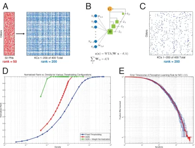
Figure 2-2 Full-rank, ultra-sparse odor representations. ... 126
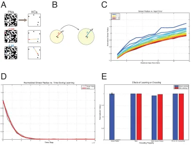
Figure 2-3 Noise robustness via Hebbian learning. ... 128
Figure 2-4 Robustness to pruning. ... 130
Figure 2-5 Proposed architecture for online learning. ... 133
Figure 2-6 Evolution of readout weights. ... 144
Figure 2-7 Mean and variance of an example readout weight. ... 145
Figure 2-8 Excitation of +bLN for 200 equiprobable inputs. ... 146
Figure 2-9 Evolution of readout weights using an actual odor encoding as input. ... 148
Figure 2-10 Mean and variance of an example readout weight when using actual odor encodings as input. ... 149
Figure 2-11 Excitation of +bLN using an actual encoding of 200 equiprobable excitatory odors. ... 150
Introduction
Olfactory computations are interesting to study for several reasons. As primarily visual animals we maybe tempted to study the visual system, but olfaction is in some ways an easier computation than vision because the anatomical structure of olfactory circuits discards most if not all of the spatial information, doing away at a stroke with the problems of rotation and translation invariance that visual systems must solve: object recognition is reduced to histogram recognition. Second, olfactory systems are grossly similar across phyla (Eisthen, 2002), suggesting the existence of an optimal method of processing olfactory signals that has repeatedly been found by evolution, and can perhaps be derived from first principles. Third, the similarity across phyla means that the insights we gain in studying olfaction in the ‘simpler’ circuits of insects are likely to generalize to the circuits in more complex animals.
ratio if the olfactory receptors are far enough apart to experience uncorrelated noise. It is currently not known whether this rule also holds in locust.
Glomeruli are sampled by the ~ 830 projection neurons (PNs) and ~ 300 inhibitory local interneurons (LNs) of the antennal lobe. The PNs are spiking neurons and form the sole output of the antennal lobe. Locust LNs are non-spiking, unlike those in bees and flies. The PNs and LNs both sample the glomeruli directly and are also densely interconnected in a recurrent circuit that produces oscillations when excited by olfactory input (Laurent and Davidowitz, 1994). Inhibition is thought to contribute to gain control and decorrelation of PN odor responses (Bhandawat et al., 2007; Mazor and Laurent, 2005), and to increase the precision of PN responses (Bazhenov et al., 2001) to presumably facilitate learning and memorization downstream.
Kenyon cells interact indirectly via the action of the giant GABA-ergic neuron, which samples the entire KC population and provide global feedback inhibition to the mushroom body (Papadopoulou et al., 2011), presumably to help maintain the sparseness that characterizes KC odor responses (Perez-Orive et al., 2002). This global feedback by the GGN will play a key role in the model circuit we propose.
readily extracted. However the nonlinear nature of LLE made it difficult to translate the results directly into the desired readout.
Summary of Contributions
for any given KC response. Conversely, I found a fixed basis in which PN responses could be reconstructed as linear combinations of KC responses, and used it to reconstruct PN trajectories from the KC data. My contributions to the paper are shown in Figures 1-2G to 1-2M, Figure 1-3G to 1-3I, Figure 1-4A to 1-4H, and 1-4L to 1-4N, and Figure 1-6F–K. Because the work presented involved both PN and KC aspects of the data, the entire paper in its current state of revision has been provided to supply the necessary context.
Chapter 1:
Encoding of Odor Mixtures:
Identification, Categorization, and
Generalization in an Olfactory System
1.1
Highlights
• We examined the responses of ~ 550 neurons (projection neurons or PNs, and
Kenyon cells or KCs) in the olfactory system of locusts to 8 single odors and 32 of their possible mixtures (of 2 to 8 components).
• Responses of single PNs to mixtures could often be at least partially explained by
responses to one of the components in mixture. The majority of PNs expressed a preference for one single component over the others. Component preference was distributed among the PNs and was different between the binary mixtures and complex mixtures experiments, suggesting PN adaptation.
• PN encoding space for binary mixtures did not appear to be discretized, and
ordered by odor similarity, and population response vectors reflected similarity for several seconds following stimulus offset.
• The responses of many KCs signaled the presence of single odor components in
mixtures, even when those single odors were part of an 8-component mixture. Individual KCs were significantly better classifiers for single odor components than individual PNs.
• Linear classifiers trained on instantaneous PN and KC population activity patterns
performed odor identification, categorization, and generalization with high accuracy.
1.2
Summary
constraints to keep representations sparse while optimizing for odor memorization, identification and generalization. These rules may be relevant for pattern classifying circuits in general.
1.3
Introduction
comprise many components, usually mixed in particular ratios. Mixtures can be perceived as wholes (“coffee”, “grapefruit”) (Jinks and Laing, 1999), but they can also be classified into categories, with various degrees of refinement (“fruity” → “citrusy” →
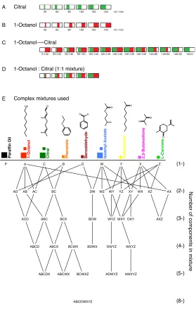
Figure 1-1 Stimulus descriptions.
For the binary mixture experiments, six different concentrations of pure citral and 1-octanol were used individually and in various mixtures. Odor pulse was 300 ms, stimulus repeated for 10 trials, each trial was 14 s. For the complex mixture experiments, 8 different molecules and a subset of their mixtures were used. Odor pulse was 500 ms, stimulus repeated for 7 trials, each trial was 14 s. (A, B) Concentrations and schematic representations of the pure odors used for the binary mixture experiments. (C) Mixture ratios used when morphing octanol to citral. (D) Mixture ratios for the concentration series experiments. (E)
Complex mixtures: Eight odor components were presented individually and in combination as 2-, 3-, 4-, 5-, 8- mixtures. Paraffin oil was also presented. In addition, three individual components (1-octanol, citral, isoamyl acetate) were also presented at 4x the component concentration, comparable in concentration to 4- mixtures. Right most column (1-, 2- ,3-, 4-, 5-, 8-) indicates number of components.
(1-) (2-) (3-) (4-) (5-) (8-) E Complex mixtures used
Number of components in mixture
30 60 80 100 120 140 ml / min
30 60 80 100 120 140 ml / min
0:140 30:140 60:140 80:140 100:140 120:140 140:140 140:120 140:100 140:80 140:60 140:30 140:0
1-Octanol : Citral (1:1 mixture) 1-Octanol Citral
1-Octanol Citral D C B A Citral
Paraffin Oil 1-Octanol Phenetole Benzaldehyde Isoamyl
Acetate
2,3-Butanedione
2-Nonanone L-Carvone
P A C B D W Y X Z
AD AB AC BC DW WZ WY YZ XY WX XZ AX
ACD ABC BCX BDW WYZ WXY DXY AXZ
ABCD ABCX BCWX BDWX DWYZ WXYZ
ABCDX ABCWX BCWXZ ADWYZ AWXYZ
1.4
R
esults
1.4.1
Definitions
Our primary data are neural responses to odor mixtures of up to 8 pure components. We define the segmentation of an odor mixture by an observer as its decomposition into its pure components. (We will describe a neuron as an odor segmenter for pure component X if its output in response to a mixture indicates the presence of X in the mixture). We define categorization as the grouping of a set of mixture stimuli based on the presence or absence of a particular odor component. Generalization is the correct categorization of a previously unknown stimulus, based on similarity to known stimuli.
1.4.2
Representations of Binary Mixtures by
Single
PNs
We first examined the responses of single PNs to binary mixtures of octanol and citral. Figure 2A shows the response of a sample PN to the mixtures tested. The responses are mixture specific, reliable, and temporally patterned, as previously observed for PN odor responses (Perez-Orive et al., 2002; Stopfer et al., 2003).
We examined the extent to which mixture responses (of single PNs) could be explained by component responses. The insets in Figure 1-2A, C illustrate that mixture responses can deviate from the arithmetic sums of the corresponding component responses. We therefore tested whether weighted sums of the form
fit(t) = a octanol(t) + b citral(t) + c,
Model Constraint
Constant a = b = 0 Unit Citral a=1, b=0. Unit Octanol a=0, b=1. Unit Mixture a=1, b=1. Scaled Citral b=0. Scaled Octanol a=0. Scaled Mixture a=b.
Free Mixture No constraints.
We allowed the component responses used a temporal jitter of up to 3 time bins. We fit all mixture responses of every PN to each one of these models and used Bayesian model selection to select the best model while simultaneously penalizing complexity (see Methods for details).
The results are shown in Figures 1-2G–M. The top panel in Figure 1-2G shows the result of the fitting procedure when applied to the response of the PN in Figure 1-2A–F to the mixture cit140:oct140. The mixture response is in black and component responses are in red (oct140) and green (cit140). The best fit selected for this mixture response was a scaled and lagged version of the response to citral. This produces an adequate fit (R2 = 0.42). The
Comparing Figures 1-2H and 1-2J suggests that non-constant fits were found whenever the response SNR was sufficiently high. Non-constant models fit approximately 62% of responses in the mixture morph experiments overall, but 89% of those for which response SNR > 3 dB (mean energy of deviations from baseline twice that at baseline). The mean ± SEM of R2 was 0.35 ± 0.01 overall, but was 0.53 ± 0.01 when response SNR > 3 dB. Thus in most cases where a PN responded reliably to a binary mixture, the response to that mixture could be explained in terms of the component responses in a manner that accounted for more than half of the response variance, on average.
Figure 1-2K shows the distribution of best models for the mixture responses of citral-, octanol-, and mixture-type PNs. For all three response-types, the majority of responses were best fit by scaling the inputs. The mean and standard deviations of the scaling factors were (0.54, 0.26), (0.51, 0.17), and (0.54, 0.18), respectively, with less than 5% of values less than zero or greater than 1. Hence most responses were best fit by scaling one of the components or the sum of the two responses by about half. We then asked whether there is an effect of mixture composition on the scaling coefficients. At each dilution, we looked for all citral-type PNs that produced a citral-type response at the dilution in question as well as at cit140:oct30 (the mixture closest to citral), and subtracted the scaling factor of the latter from the former, including unit-type responses in this analysis with a scaling factor of 1. We repeated this procedure for the octanol type responses. In Figure 1-2L, the mean and S.E.M.s of these differences are plotted as a function of dilution. The data have been rearranged to plot the same relative dilution at the same x-value for both citral- and octanol-type responses, so that the citral-octanol-type values plotted at 140:60 are for the cit140:60oct, while the octanol type values plotted are for the cit60:oct140 mixture. Stars indicate significant differences from zero (p < 0.05, paired t-test), indicating increased suppression as the concentration of the complementary odor is increased. An overall trend with mixture dilution was present in both traces, and could be fit with sinusoids (citral: R2 = 0.92, p < 10
-5; octanol: R2 = 0.76, p < 10-3). This analysis shows an increase in suppression of the
were reversed. These observations may be single-neuron hallmarks of gain control in the antennal lobe.
As shown in Figure 1-2H, the majority of binary-mixture responses were best fit by scaling the response to one or the other component; true mixture-type responses were relatively rare. This could have resulted from the suppression of the response to one of the components when presented in the mixture, indicating a strong nonlinearity. But this result could have other explanations: for example, if a PN responded to both components but to each with very similar response profiles, only one would have been selected to contribute to the mixture fit, causing the other to be artificially eliminated during model selection. We thus computed the ‘SNR-angle’ of each fit response. The SNRs of the component responses were computed as for the response SNR, substituting the component responses for the mixture response. The resulting two SNR values (in dB) defined a 2D vector whose angle to the x-axis we define as the SNR angle: an angle of zero indicates a response to octanol and no response to citral; an angle of π/2 indicated the converse. In Figure 1-2M
we plot the histogram of these angles for the different response types. It shows that the majority of octanol-type responses have an SNR angle near zero, while the majority of citral-type responses have an angle of near π/2. This indicates that many citral- and
Figure 1-2 PN responses to binary odor mixtures can exhibit nonlinearities.
column, citral-type PNs are in the right, and mixture-type PNs are in the bottom grid, along with two PNs in which neither citral or octanal type responses dominated. (I) Fit quality. Grids are arranged in exactly the same way as in (H), but colored according to the R2 value of the fit from red to blue according to the legend at the top. (J) Mixture response SNR. Grids are arranged exactly the same way as in (I) and (J), but colored according to SNR(dB) according to the legend at the top. Black indicates 0 dB: mean response energy is equal to mean baseline energy. Dark-red is 3 dB: mean energy of response deviation from baseline mean is twice that at baseline. Comparing this panel to the previous two shows that high SNR typically produced good quality fits, and conversely. (K) Distribution of the forms of the models fit for each type of response. 1-: unit model, the fit is equal to the component response (or the sum of the component responses for mixture-type responses) plus a constant offset; k-: scaled model, the fit is equal to a scaled version of the component response (or the sum of the component responses for mixture-type responses); f: free model – the fit was an unconstrained linear combination of the component responses; -lag: At least one of the components used was lagged in time. Note the predominance of the scaled model in all three types of responses. (L) Effect of the mixture on the scaling factor of the fits. The change in the scaling coefficient relative to the value at the strongest dilution as a function of the mixture is plotted using data from all citral-type and octanal-type PNs. The data have been rearranged so that the x-axis labels correspond to the same dilution for each type of response, e.g., the data plotted at 140:60 correspond to cit140:oct60 for the citral data, and cit60:oct140 for the octanal data. Error bars are ± 1 S.E.M. Stars indicate significant difference from zero (p < 0.05, paired t-test). Dashed lines are sinusoidal fits (citral: R2 = 0.92, p < 10-5; octanol: R2 = 0.76, p < 10-3). (M) Smoothed histogram of SNR angles for mixture responses of each type. Values near 0 indicate that the corresponding response to pure citral was very weak relative to the response to pure octanal, and vise-versa for values near π/2. Note that that most octanal-type
responses cluster around 0, and most citral type responses cluster around π/2, indicating a lack of response
1.4.3
Representations of Binary Mixtures by
PN Populations
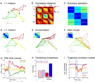
Because odor representations by PNs are highly distributed and varied in time (Figure 2 and (Laurent and Davidowitz, 1994; Mazor and Laurent, 2005; Stopfer et al., 2003)), because their activity patterns are decoded by individual KCs on which converge many PNs (Jortner et al., 2007) and because KCs have very short effective temporal integration windows (Perez-Orive et al., 2004; Perez-Orive et al., 2002), it is useful to examine PN responses as time-series of instantaneous population vectors, or trajectories, and visualize them in an appropriately reduced state space (Broome et al., 2006; Brown et al., 2005; Mazor and Laurent, 2005; Stopfer et al., 2003). Figure 1-3A illustrates these PN population trajectories in response to 1-octanol (red), citral (green), and their 1:1 mixture (yellow), after dimension reduction by locally linear embedding (LLE) (Roweis and Saul, 2000). The non-linear nature of LLE makes quantitative comparisons between trajectories difficult. Therefore, we also show correlation measures between the trajectories in the full space. The nine matrices in Figure 1-3B plot the correlation distance (Dc, see Methods) within
1-4A–C). The combination of correlation measures and LLE trajectories provide both quantitative and qualitative descriptions of the data.
the PAF for the 1:1 mixture mostly stays near 0.5, and the low variability indicates that this value is stimulus-driven and not simply due to noise. The PAFs computed with respect to octanol were equal to 1 minus the PAFs to citral, and nearly 75% of the magnitude of the population vector lies in the projection during the early phase of the response (Figure S1-3). Hence we conclude that the trajectory for the 1:1 mixture indeed lies almost exactly in between the trajectories for the two components.
Figure 1-3E represents concentration series for the three stimuli (cit, cit:oct, and oct). Extending previous results (Stopfer et al., 2003), we find that concentration series for 1:1 mixtures, as for single odors, generate families of closely related trajectories (lower-dimensional manifolds), clustered by odor rather than concentration (see also matrix inset). We quantified this impression by computing Rand indices (Rand, 1971) globally on the full-space data, measuring the agreement between clustering by correlation distance and clustering by odor, or between clustering by correlation distance and clustering by concentration (Figure 1-3H, see Methods for details) (range 0–1, higher meaning better agreement). At baseline, both comparisons yielded values close to chance (dashed line). During the response window, clustering was clearly by odor (Figure 1-3H).
one odor appeared to shift gradually towards that for the other odor, passing through their 1:1 mixture trajectory. We quantified this impression by fitting, in consecutive 100 ms time bins, the correlation distance between each PN vector (full space) for the mixture and that for citral, as a function of the concentration ratio (log10 of the ratio of the
Figure 1-3 PN representations of binary mixtures are structured.
(A) Dimension reduced (LLE) population trajectories in response to pure citral (140 ml/min, green), pure octanol (140 ml/min, red), and the 1:1 mixture (yellow). (B) Correlation distances between average PN activity patterns in trials 3–6 and trials 7–10 evoked by pure citral, pure octanol, and the 1:1 mixture in adjacent 50 ms time bins in the 3 seconds following odor onset. The color range has been clipped from [0– 2] to [0–1] for clarity. (C) The data in (B) is summarized by taking the minimum over each of the 9 odors comparisons. Colors are the same as in (B). (D) Same as (A), but now with correlation matrix inset as in (C). (E) Concentration series trajectories and correlation summary matrix. Concentrations were 30, 60, 80, 100, and 140 ml/min of citral (dark to light green), octanol (dark to light red), and the 1:1 mixture (purple to yellow). (F) Trajectories and correlation summary as pure citral (green) is morphed to pure octanol (red). The concentrations used were 140:0, 140:30, 140:60, 140:80, 140:100, 140:120, 140:140, 120:140, 100:140, 80:140, 60:140, 30:140, 0:140 in units of ml/min citral : ml/min octanol. (G) Mean (traces) ± S.E.M. (bands) over trials of the projection angle fraction (PAF) relative to citral in 100 ms time for ‘mostly octanol’ (red), 1:1 mixture (yellow), ‘mostly citral’ (green), computed in the full (non-dimension-reduced) PN space. Concentrations were 30:140, 140:140, and 140:30 in units of ml/min citral : ml/min octanol, respectively. The PAF for the 1:1 mixture remains close to 0.5 after onset, indicating that its trajectory lies almost exactly in between that of citral and octanol, confirming the impression from (A, D).
1.4.4
Representation
s
of
Complex
Mixtures by Single PNs
Eight molecules were chosen to be chemically distinct (Figure 1-1E) and their concentrations adjusted to evoke electro-antennograms that were reliable, small and comparable in amplitude (Figure S1-1C, D), to compensate for differences in vapor pressure or receptor activation and to ensure operation far from saturation. As done with the responses of single PN to binary mixtures, we determined the extent to which the mixture responses of single PNs could be explained in terms of their responses to the single components in the mixture. The response of a PN to an n-component mixture was regressed on the constant model (no inputs), and all 2n - 1 possible combinations of single component responses. For each such input combination, we computed the regression for the unit-, scaled- and free-coefficient models, as well as for lagged versions of these. We then determined the best model using Bayesian model selection (see Methods).
but each grid cell is colored according to the quality of the corresponding fit measured using the R2 value of the fit according to the color scale shown at the top. Figure 1-4D,
again arranged as Figures 1-4A–B, encodes response SNR, computed as for binary mixtures, and colored according to the scale on top.
Overall, best fits involving one or several components were found for 31% of the PN-mixture conditions. Comparing Figures 1-4B and 1-4D suggests that such fits were possible whenever the SNR was sufficiently high (61% of PN-mixture conditions in which SNR > 3dB). The mean ± SEM of R2 overall was 0.15 ± 0.0034, but 0.30 ± 0.0050 when
SNR > 3dB. These values are significantly lower than for the binary mixture experiments (0.35 ± 0.0075, and 0.53 ± 0.0080, respectively, see above). We also compared the results of two sets of separate experiments directly (i.e., based on different PN recordings) at the mixture condition they had in common (cit100:oct100), tested in the binary mixture concentration series experiments and called odor AC in the complex-mixture experiments. In the latter, 21% of PN responses to AC could be fit to a non-constant model (45% of those in which response SNR > 3 dB). In the binary-mixture experiments, 60% of cases of odor AC could be fit overall (85% of those above 3 dB).
For each PN, we computed the maximum SNR of its component responses, and the SNR of its mixture response. We then categorized the PN responses into four groups based on their component and mixture responses being above or below 3dB: (1) Silent: Component and mixture SNR < 3 dB; (2) Suppression: Component SNR > 3 dB, mixture SNR < 3dB; (3) Emergent: Component SNR < 3dB, mixture SNR > 3 dB; (4) Full response: Component and mixture responses > 3dB. The percentages of PNs with suppression- or emergent-type responses were similar in the binary mixture and complex mixture experiments: 4.2%, and 15% for suppression- and emergent-type responses in the former case, vs. 8.0% and 19% in the latter. A large difference was found in the percentage of silent cells: 24% for cit100:oct100, vs. 47% for odor AC. This suggests that the main reason for an overall lower fraction of responses that could be fit in the complex mixture conditions is that these mixture conditions engaged fewer cells, possibly due to adaptation. Note that this explanation does not account for the lower fraction of responses above 3 dB that could be fit in the complex mixture conditions, which must be due to an increase in gross nonlinearities in the complex mixture conditions. These results will be examined in the Discussion.
Such a distribution of response types would allow both concentration-invariant and concentration-sensitive types of olfactory computation. Note also that some PNs have a secondary preference. For example, there is a C-type PN that has a secondary preference for component W (a “Cw” type response), a W-type PN with a secondary preference for component C (a “Wc” type response). This is particularly interesting because these components are chemically similar (C = citral, W = isoamyl acetate). Other pairings can also be found, such as Xw, Wb, etc.
Figure 1-4E shows the distribution of model fits for each response type. The majority of the responses were scaled (57%) and un-lagged (53%). The mean ± S.E.M. of the scaling weights computed over all such PNs for all fits using the preferred component of each was 0.72 ± 0.0093, similar to what was found with binary mixtures when pooling over the preferred-component fits for citral- and octanol-type PNs (0.74 ± 0.0034).
some mixture level). Of the 125 available PNs, we kept the 99 for which at least 3 of the 5 values were available. The data for these PNs are plotted in Figure 1-4F according to their preferred odor component; no clear trend could be detected. We then computed the Spearman rank correlation of scaling coefficient with the mixture level for these PNs. For 8 of the 99 PNs there was no change in scaling coefficient with mixture level, and to these we assigned a correlation value of 0. The mean and median of the correlation coefficients were -0.15, and -0.20, respectively, suggesting a slight negative trend, though it was not significant (median not significantly different from zero; p-value = 0.093, sign-test). Hence, PNs “preferring” a single component will respond to mixtures containing their preferred component by scaling their component response to ~ 3/4 of its unmixed magnitude, on average.
Finally we examined the extent to which a PN’s mixture response best explained by a particular component implied a suppression of the other component responses. For each of the 1545 responses that were fit by single components (of 5600 total), we computed the SNR of the response to the favored single component, and the maximum SNR of the responses to the other components present in the corresponding mixture. We thus positioned each response in 2D space, and computed the SNR angle such that an angle near zero meant that the preferred response was much stronger than all of the others, while an angle near π/2 meant that at least one of the component responses was much stronger than
clear peak near 0 degrees, and only a small one near π/2. However, there is a large
secondary peak near π/4, suggesting that in many of the responses fit by a single
component, at least one secondary component was suppressed, or had a response time course sufficiently similar to the preferred component that its contribution to the fit was minimal. Limiting the analysis to the 917 responses from A- to Z-type PNs that were fit by their preferred-components slightly increased the height of the peak at zero (red curve), reduced the one at π/2, but did not alter that at π/4. The preferred component was dominant
(|SNR angle|<π/8) in only about half of the responses (42% overall, 49% for
preferred-component responses). These values are lower than those (66%) for the binary-mixture experiments, indicating that component suppression (or redundancy) is greatly increased in the presence of complex mixtures.
The SNR angle cannot distinguish between a secondary component response that is not included in the fit because it appears redundant (e.g., present but similar to and overlapping with the response to the primary component), and one that is actively suppressed. To make this distinction we examined all 184 cases in which π/8 < SNR < 3π/8 , i.e., those for
ratio of the weight for the fit using the secondary component to that using the primary component. Values range from -0.5, indicating strong suppression, to ~ 1, indicating redundancy. We took the threshold between suppression and redundancy to be the dashed line at a ratio of ~ 0.2 because manual inspection of the fits showed that when the ratio was small but positive, the best fit was essentially a constant function. 67% of the fits were below this threshold, indicating an active suppression of the secondary component. The mean ± S.E.M. of the correlation coefficient between the primary and secondary component responses in these cases was -0.10 ± 0.017, and -0.12 ± 0.012 between the secondary component and the mixture response. For the 33% of cases in which the responses were above threshold (i.e., redundant), the mean ± S.E.M. was 0.37 ± 0.031, and 0.36 ± 0.021 between the second component and the mixture response. Thus, when the fit considering a secondary component required only a moderate scaling, that component response was positively correlated with that to the primary component; conversely, when the fit required a suppression or subtraction of the secondary component response, the correlation was weak and/or negative, as should be expected.
1.4.5
Representations of Complex Mixtures by PN Populations
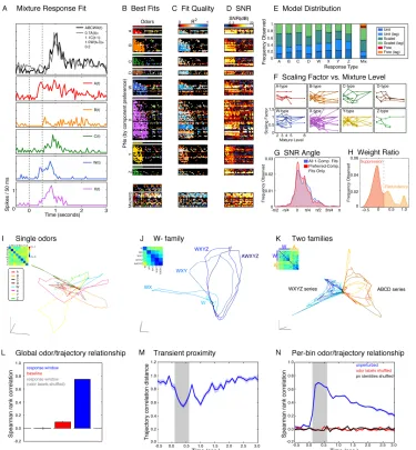
The LLE trajectories corresponding to the eight component odors are shown in Figure 1-4I. Consistent with the odors’ distinct chemical composition, these trajectories did not cluster (see also minimum correlation distances in inset). The observed lack of clustering suggests large differences between the evoked PN response patterns, as desired. Adding components to a single odor, W (Figure 1-4J), caused the mixture trajectories to deviate from that for W. Incremental changes in the population trajectory, however, decreased as the number of components in the mixture increased (see also minimum correlation distance matrix). This is consistent with the fact that the fractional change to the stimulus decreased with each single component addition. This observation was repeated with the other odors and quantified by analysis in full PN space (not shown).
These results suggest that the representations of complex mixtures by PNs are ordered: the more similar odors are, the more similar their corresponding representations by PNs. To test this hypothesis, we computed the dissimilarity between odors (represented as 8D binary vectors whose coordinates indicate the presence or absence of each of the 8 components) using the Jaccard distance (Deza and Deza, 2009). We computed all pairwise distances Dj between odors, and all correlation distances Dc between the PN population
vectors corresponding to those odors (calculated globally over the entire response). In Figure 1-4L, we plot the Spearman rank correlation between Dj and Dc calculated over the
response (blue), over baseline (red), and a control (gray). During the response window there is a strong tendency for trajectory distances to increase with odor distances, while during baseline this trend is very weak (see also Figure S1-4). We conclude that the evolving odor representations by the PN population continuously contain information about stimulus composition in their global inter-trajectory distances. When observed bin-by-bin, distances between trajectories can vary: Figure 1-4M, for example, shows the evolution of Dc calculated for odors WYZ and DWYZ over time. But information about odor
Figure 1-4 PN representations of complex mixtures reflect odor similarity.
(A) Example mixture response fit. Response (mean firing rate in adjacent 50 ms bins) of a cell to the 5-component mixture ABCWX (black), and the best fit (gray). Dashed lines indicate the odor window. (B)
stacked bar plot shows the relative frequency of unit- and scaled-coefficient models used in the corresponding single component fits, and also the distribution of free-coefficient models used in fits where more than one component was used. (F) Scaling factor in fits as a function of mixture complexity. Each panel plots the variation of the mean scaling factor used in the corresponding single component fits as the mixture level is increased. Only PNs are used which had at least one preferred-component response in at least three mixture levels. No obvious trend with mixture level is present in any of the panels. (G)
Smoothed histograms of SNR angle computed over all single-component fits (blue), or limited toPNs with a preferred component, for fits using that component (red). Angles near 0 indicate that the single component response for the component used in the fit was dominant; those near π/2 indicate that a
secondary component response was dominant; those near π/4 indicate that the primary component response
was approximately matched in SNR by at least one of the secondary responses. (H) Smoothed histogram of the ratio of the scaling weight for the best single component fit using the secondary component, to that when using the primary component, for the fraction of data points whose SNR angle (red curve in panel G) was near π/4. Values below 0.2 were likely to be actively suppressed in the mixture response; those above
1.4.6
Kenyon Cell Responses to Mixtures
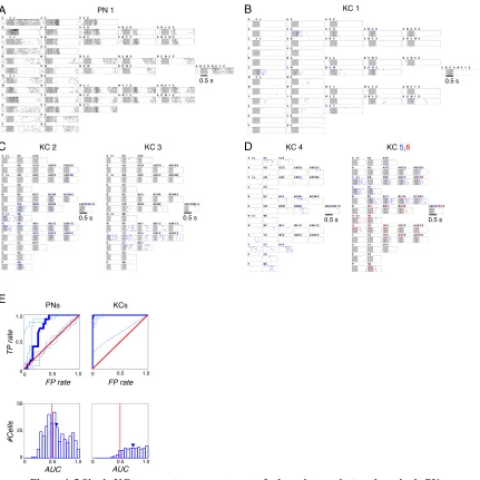
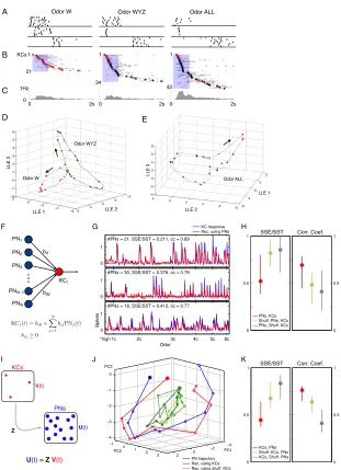
Figure 1-5 Single KCs segment components out of odor mixtures better than single PNs. (A) Spike rasters of a representative PN to single and mixed odors (see Methods for 44 stimuli, 7 trials, 500 ms stimulus at shaded area, 2.5 s shown). Numbers of components organized by column, conditions arranged to make overlapping mixtures adjacent wherever possible. (B–D) Spike rasters of six representative KCs. (B) D-segmenting KC, with weak late response to unrelated mixtures Y, WZ, YZ. Same scale as in (A). (C, D) Other representative KCs, showing segmentation of different odors (in order of KCs: W, Y, X, C and W). KCs 5 and 6 recorded simultaneously; both responded to mixtures containing both C and W (e.g., BCWX), but at different times. Only 1 s shown, centered on KC response times; Time scale as in (B). (E) Top panel: ROC evaluation of component selectivity by PNs and KCs. True and false positive rates (TP, FP) determined by sliding response threshold; response based on spike counts within 1 s window summed over 7 trials. Red diagonal: chance performance. Blue lines: results for several example PNs (the curve for the PN 1 is highlighted), and for the KCs in (B–D) (the curve for KC 1 is highlighted; see Methods for class partitions). Bottom panel: Distribution of area-under-curve (AUC) values for KC-odor class pairs significantly shifted to the right of PN-KC-odor class pairs (p < 10-7, Wilcoxon rank sum test). Arrows indicate means: 0.74 (KCs; SD = 0.17); 0.59 (PNs; SD = 0.20).
A PN 1
0.5 s
B KC 1
KC 4 KC 5,6
PNs KCs
KC 2 KC 3
C D E FP rate FP rate T P rate AUC #Cells AUC 0.5 1.0
0 0 0.5 1.0
0 50 25 0 1.0 0.5 0.5 1.0
0 0 0.5 1.0
0.5 s
1.4.7
Decoding PN
T
rajectories
O
ver
Time
If single KCs decode PN trajectories, then, given our large dataset of PNs, we should be able to use PN responses to reconstruct those of the KCs. To test this possibility, we formed odor response vectors for each PN and KC by computing its average spike count binned in 100 ms bins in the 1 second window following odor onset, and concatenating across the 44 odors tested. This yielded, for each PN and each KC, a 440-element (10 bins x 44 odors) response vector. We then used the multi-stage adaptive lasso (Buhlmann, 2011) to linearly regress the response vector of each KC on those of the PNs, while constraining the regression weights to be positive, to reflect the excitatory nature of connections from PNs to KCs (Jortner et al., 2007). This is shown schematically in Figure 1-6F.
Figure 1-6G shows three of the best reconstructions: in all three, more than half of KC-response variance could be explained using 30 or fewer of the 175 available PNs. Figure 1-6H summarizes the distribution of reconstruction results over the KC population. The median value of the fraction of variance un-explained (SSE/SST) is 0.52. Twenty six percent of the KC responses could not be regressed at all on the PN responses. The mean ± S.E.M. of the number of connections used in the remaining reconstructions was 10±0.6, with a maximum value of 30.
Methods for details). If shuffled PN responses were used (with the same number of regressors as in control), the median of the SSE/SST distribution was 0.82, indicating a significant loss in performance. Conversely, we used the PN responses to reconstruct the shuffled responses of KCs, yielding a median value of SSE/SST of 0.86, again, indicating a loss in performance. In short, our results show that the responses of single KCs can be reconstructed from pooled subsets of PNs, consistent with the cycle-by-cycle decoding of the PN population by KCs.
unexplained (SSE/SST), and then averaged this value over the trajectory. The distribution of mean values over the 44 odors is plotted in in red. The median value was 0.44, the value for the example shown in Figure 1-6J. Similarly, we computed the mean over time bins of the correlation between the trajectories and their reconstructions (red, right panel of Figure 1-6K). The median was 0.76, the same as that for the example in Figure 1-6J.
Figure 1-6 Distribution of KC response times.
(A) KC rasters in response to W, WYZ and ALL (ABCDWXYZ). KCs respond reliably across trials and differ in response duration and timing. (B) Activity of all recorded KCs that responded to W, WYZ, and ALL. Gray: PSTH averaged across 7 trials, normalized between 0 and 1; dots denote peak of corresponding PSTH. KCs ordered by time of peak, illustrating sequential spread of activity, especially tight within first 500 ms. Red dots: W-responding KCs; black dots: KCs that did not respond to W presented alone. Shaded bar: odor, 500 ms. (C) Instantaneous firing rates, averaged across all trials and all 209 KCs to W, WYZ, and ALL. Values are greater with larger mixtures because, on average, more KCs respond to a mixture than to individual components. (D, E) Two-trial averages of LLE trajectories evoked by W, WYZ and ALL, analyzed over 175 PNs (50 ms consecutive bins, 4.5 s from odor onset), plotted in LLE 1–3 space. LLE computed separately for (D) and (E) (i.e., different coordinates) and plotted separately for clarity. KC PSTH peaks from (B) are superimposed on PN trajectories at corresponding times. (F) Schematic representation of PN trajectory reconstruction from KC responses. We searched for a fixed PN x KC basis matrix Z which would transform instantaneous KC population response vectors V(t) into the simultaneous PN population response vectors U(t). (G) Example trajectory reconstructions. The PN population trajectory in response to odor ABC is shown in PCA-space in blue. The fit using the KCs is shown in red. Three
Odor W Odor WYZ Odor ALL
1Hz 0
0 2s
1 1 1
21
34
43 KCs
0 2s 0 2s
A B C Odor W Odor WYZ D
LLE 1 LLE 2
LLE 3 Odor ALL E LLE 1 LLE 2 LLE 3 0 0.5 1 KCs, PNs Shuff. KCs, PNs KCs, Shuff. PNs
0 0.5 1
KCs
PNs
U(t) = Z V(t)
V(t)
U(t) Z
I J K
−4 −2 0 2 −1 0 1 2 3 −4 −3 −2 −1 0 PC1 PC2
PC3 SSE/SST Corr. Coef.
PN trajectory Rec. using KCs Rec. using shuff. KCs 0
1
#PNs = 21, SSE/SST = 0.211, cc = 0.89
0 1
#PNs = 30, SSE/SST = 0.376, cc = 0.79
*high 1c 2c 3c 4c 5c 8c 0
1
#PNs = 18, SSE/SST = 0.412, cc = 0.77
0 0.5 1
PNs, KCs Shuff. PNs, KCs PNs, Shuff. KCs
0 0.5 1 PN1 PN2 PN3
PNN -1 PNN
KCi
bi1
biN
F G H
SSE/SST Corr. Coef.
Odor
KC response Rec. using PNs
1.4.8
Odor Identification, Categorization, and Generalization
from
P
opulation
A
ctivity
Because KCs are in turn read out by downstream decoders (Cassenaer and Laurent, 2007, 2012; Heisenberg, 2003; MacLeod et al., 1998; Masse et al., 2009), we examined the information present in the KC population vectors in appropriately short time bins. Using a linear classifier (regularized-least-squares, see Methods), we compared the decoding of odor identity, category and generalization using instantaneous PN and KC population output. Decoding accuracy in the identification and categorization tasks was based on trials excluded from the classifier training; for the odor generalization task, all trials with the tested odor were excluded from training. Thus, the measured accuracy was what real downstream neurons might achieve in single trials by computing a weighted sum of spikes in each measurement bin (see Methods). Identification required attributing a particular KC or PN response vector to the correct odor (all-vs-all, 44 classes, chance = 2.27%). Categorization consisted in discriminating mixtures containing a given component from
Figure 1-7 PNs and KCs can be linearly decoded to perform odor identification, categorization, and generalization.
1.5
D
iscussion
1.5.1
Mixture Representations by Single PNs are Partially
Explai
ned by the Responses of those PNs to the
Components
By linearly regressing the mixture responses of PNs on to their component responses, we found that the component responses could explain a significant fraction of the mixture response variance, particularly when a clear mixture response was present: ~ 50% in the binary morph experiments, and ~ 30% in the complex mixture experiments. Most fits used only a single component response, even for complex mixtures. This enabled us to decompose the PN population for each experiment by component preference, showing both that each component is represented in the population, and that a full spectrum of dilution sensitivity exists for each component. Such a distribution of response profiles would clearly facilitate olfactory computation.
with relatively few responding to both. In the complex-mixture condition, we examined the ~ 20% of cases in which at least two equally strong component responses were present but only one was ultimately used in the fit. We found that in 2/3 of cases this was because the second component was poorly correlated with the response and was likely to be physiologically suppressed. In only about 1/3 of cases did we observe a response strongly correlated with the primary component response, and that may have been rejected by the fitting procedure due to its redundancy with the primary response, thus potentially hiding a true mixture response. We also checked many of the fits “manually”, especially those with high response SNR that were poorly fit by single components, inspecting the models considered and the models finally selected. These inspections almost always confirmed the decision made. The procedure itself also had very few parameters and required very little tuning. Thus, we believe that the model selection procedure did not introduce an unjustified bias against mixture responses.
found for three times as many mixture responses in the binary morph experiments as in the complex-mixtures experiments. A possible explanation is that the antennal lobe tuned its sensitivity to the odors encountered most often during the course of each experiment. The fact that we found more PNs sensitive to the component most commonly used in mixtures (2,3 butanedione) is consistent with this explanation.
1.5.2
Odor Representations by PN Populations
a
re Ordered
With more complex mixtures, we found a positive correlation between chemical similarity (i.e., the number of shared mixture components) and representation similarity. This was true whether representations were measured over the entire response window or piecewise, over individual time bins. While such a relationship might have been expected very early in the response, when PN activity is dominated by receptor input, we observed that it obtains throughout the odor presentation and for several seconds following odor offset. Together these results indicate that odor representations are not randomly distributed in PN space, but are ordered so that chemical similarities are reflected in similarities in the evoked neuronal activity patterns. While random representations can in principle be as useful as ordered ones for the decoding of odor identity by downstream cells, ordered representations can make the computation of categorization and generalization easier by representing similar odors in similar ways, and may be the substrate for the categorization and generalization performance we observe in KCs, the PNs’ targets in mushroom bodies.
1.5.3
Subspace Readout of PNs by KCs
approximately eight ways according to component sensitivity. Assuming some redundancy between the responses of PNs within a group, a small number of ‘basis-PNs’ would be required to capture the variability of all the responses within the group, and only those PNs would show up in the regression (due to the sparsity prior of the lasso). Thus this low apparent connectivity could be explained by the redundancy of PN responses.
1.5.4
Individual KCs are Better Odor Segmenters than Individual
PNs
Surprisingly, Kenyon cells—which are directly postsynaptic to PNs—are individually much better than PNs at detecting a component in a mixture of up to eight odors (ROC analysis). This observation might be explained using a simple abstraction: odor representations are spread orderly in a high-dimensional PN space (Figure 1-3,1-4); because of their 50±15% connectivity to PNs (Jortner et al., 2007), however, the KCs each
more likely to respond to a mixture if it had first been exposed to a component of that mixture.
1.5.5
Population Decoding from PNs and KCs
Our results (Figure 1-7, S1-7) show that both the PN and KC populations can be read out by linear classifiers in single time bins to perform odor identification, segmentation, and generalization, and that the time course of the performance is similar in both populations. Although we sampled ~ 20% of the full PN population, but only ~ 0.4% of the KC population, readout performance from KCs was usually only slightly worse than from PNs. One explanation for this observation is that by pooling information across the PN population, individual KCs are more informative than individual PNs. However, another explanation is that our bias in KC selection due to experimental design may have skewed our KC dataset towards particularly informative cells. The collection of larger and less biased KC datasets will be needed to elucidate this point.
1.5.6
Experimental Sampling
Bias
search was done using only the eight single odors in our stimulus set. As soon as high S/N signal was detected on at least one tetrode in response to at least one of the eight odors, the experiment could commence. Our KC dataset is thus somewhat biased towards KCs that respond to the odors present in our single-component stimulus set. In a typical recording session, however, it was common to record KCs that did not respond to any of the single components. Among those were some that responded to “low-n” mixtures—two or three components. Those KCs then often responded to high-n mixtures containing the low-n ones, practically segmenting these lower-order mixtures, just as other KCs detect single components. Hence, while our KC data are biased towards KCs that responded to the 8 single components in our stimulus set, it contains no experimental bias towards mixture-responsive or component-segmenting KCs, for those were all discovered post-hoc, during data analysis. It is possible, however, that our initial screening procedure with the eight single odors introduced an acquired (though unconditioned) selectivity for these components. Whether the segmenting properties of KCs we describe here are intrinsic or learned via a fast non-associative process (see, for example, (Stopfer and Laurent, 1999)) is unknown thus far.
1.5.7
Functional C
onsequences
of Odor Segmentation
expressed good segmenting properties (one KC for each one of the eight single odors). Each column represents one of the 43 stimulus conditions (paraffin oil not shown). The color of each square identifies the odor component that the corresponding KC detected. The circles indicate a response. For example, KC3 was a nearly perfect segmenter for citral, with only one false positive (last of the 3-mixtures) and one false negative (8-mixture). Thus, any odor—whether simple or composite—can be represented by a unique 8-D activity vector. The first 4- and 5-mixtures, for example, are represented by KC activity vectors that differ simply by the activation of KC6. To the limit, if every KC was a perfect detector for only one feature, then n KCs could encode 2n-1 different odor feature combinations, plus baseline (0,0,…0). By contrast, a “grandmother” scheme whereby each odor is represented by a unique neuron would require 2n-1 KCs to represent this many odors and mixtures. Hence, KCs implement a clever strategy. Odor representation is sparse (effective for memory formation and recall, yet not maximally sparse), but distributed such that the coding capacity for related stimuli (mixtures) is greatly increased.
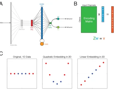
Figure 1-8 Coding principles for odor identification and generalization by KC assemblies. (A) Diagram indicating the responses of eight of our recorded component-detecting KCs (one for each of the 8 tested) to all odor conditions. Response measured as spike counts in 1 s window from odor onset summed over all 7 trials, normalized between 0 and 1 for each KC. Filled circle area represents response. Each color represents one odor. A filled circle on a colored square indicates a “true positive” (a KC recognizes the component to which it is tuned from within a mixture). An empty colored square indicates a “false negative”. Black circle alone indicates “false positive“. KC 5 detects W without mistake. In the absolute, downstream decoders need only read one KC to recognize a category: for instance, a response in KC 3 indicates the presence of odor C. Identification is possible by observing across the 8-D KC vector (e.g., discrimination between mixtures ABCD and ABCDX, vertical arrows). With perfect component-detectors, n KCs can discriminate between 2n-1 odor mixtures (all combinations) and baseline. The code is sparse for single components and more distributed (though still sparse) for mixtures. (B, C) Linear classification of odors and mixtures using ordered KC encoding scheme. Schematic of KC coding space where each KC represents an odor component. With this scheme, generalization is simple: (B) shows hyperplanes that separate mixtures into A vs. not-A, B vs. not-B, and C vs. not-C; (C) shows hyperplanes that generalize mixtures into AB vs. not-AB, BC vs. not-BC, and AC vs. not-AC. Information is represented such that different kinds of generalization are easy to compute with linear classifiers. (D–F)
1.6
M
ethods
1.6.1
Preparation and Stimuli
Results were obtained from 61 locusts (Schistocerca americana) in a crowded colony. We recorded from 168 PNs for the binary mixture experiments, 175 PNs for the multi-component mixture experiments and 209 KCs from 13 (42 groups), 11 (36 groups) and 37 locusts (53 groups), respectively. Experiments were typically conducted using left and right antennal lobes (ALs) and mushroom bodies (MBs) in each animal. Young adults of either sex were immobilized, with one or two antennae intact for olfactory stimulation. The brain was exposed, desheathed and superfused with locust saline, as previously described (Laurent and Davidowitz, 1994). Odors were delivered by injection of a controlled volume of odorized air within a constant stream of desiccated air. Teflon tubing was used at and downstream from the mixing point (see below) to prevent odor lingering and cross-contamination. Due to different odor stimulus requirements between the binary morphing and the multi-component mixture experiments, we built two independent odor delivery systems (Figure S1A,B).
1.6.2
Binary
Mixture Experiments
desiccated, filtered air. The flow of each odor was controlled by an independent electronic flow meter with feedback control (Aalborg, 2–200 ml/min) and a solenoid placed upstream of custom-made bubbler (Figure S1-1A). Relative odor concentrations were varied by controlling flow through each bubbler (30, 60, 80, 100, 120 and 140 ml/min). These concentrations spanned the dynamic range of electro-antennal responses recorded in recordings from isolated antennae (electro-antennograms, or EAGs). A large vacuum hose placed behind the antenna guaranteed the quick removal of odorants from the space surrounding the antenna. Odor puffs were triggered automatically using a custom computer interface (LabView, National Instruments Inc.). Trials were 14 s long, with 300-ms-long odor puffs presented 2 s after trial onset; each odor condition was repeated 10 times.
1.6.3
Complex
Mixture Experiments
(60 ml). The headspace content was carried by puffs of desiccated and filtered air, with a flow rate of 100 ml/min for individual odors and 400 ml/min for paraffin oil. Three odors: 1-octanol (A), citral (C), and iso-amyl-acetate (W) were also presented at a second, higher concentration, by increasing flow rate to 400 ml/min. Odor mixtures were presented by combining the single odorants. For example, AB was the combination of 100 ml/min of A with 100 ml/min of B, with a total odor flow of 200 ml/min; thus, total odor concentration was higher during mixture conditions. A compensating stream of desiccated air was used to ensure that total air-flow remained constant throughout the experiment. The odors were mixed in a custom-built corrugated glass tube (~ 8 cm long, 1.5 cm diameter), with a total flow of 2 l/min to ensure turbulent mixing. The individual odor lines were arranged along the circumference of the mixer. Trials were 14 s long, with odor puffs presented for 500 ms, 2 s after trial onset, and repeated 7 times with each stimulus. To minimize the potential effects of priming (Bäcker, 2002), single odorants were presented first, followed by 2-, 3-, 4-, 5- and 8- mixtures. The order of presentation within each mixture group was pseudo-random.
1.6.4
Electrophysiology
tip was electroplated with a gold solution to reduce the impedance to between 200 and 250 kΩ at 1 kHz. The same custom-built 16-channel preamplifier and amplifier were used for both types of tetrodes. Two to four tetrodes were used simultaneously. The preamplifier had a gain of 1, and the amplifier gain was set to 10,000x. Because of low baseline activity and low response probability in KCs, fewer KCs than PNs were usually isolated in a typical recording session. Tetrodes were placed within the AL or MB soma clusters, peripheral to the neuropils at depths between 50 and 200 µm. For some MB recordings (KCs, LFP), probes were pressed on the surface of the MB. Cell identification was unambiguous because PNs are the only spiking neurons in the locust AL—LNs do not produce sodium action potentials (Laurent and Davidowitz, 1994)—and because all the somata located dorsal to the MB calyx belong to KCs. Recording locations were tested randomly across the MB and selected if activity could be elicited by any of the 44 odor conditions. Identical stimuli were presented at the beginning, middle and end of the experiment to check that clusters had not drifted significantly over the course of the experiment. Drift was estimated qualitatively by determining if a given neuron’s responses to each odor were similar across these three sampling periods. Hints of drift then led to examination of the waveform clusters.
1.6.5
Recording
Constraints and Sampling Biases
separable PN clusters could be seen, recordings started and responsive PNs were always found. Our estimates of PN response-probabilities are therefore likely close to true values. By contrast, KCs respond very rarely to odors and responsive KCs had to be found through an active search. Experiments would commence only if a response was elicited by at least one of the 8 monomolecular odors. See the Discussion and supplementary text for more details on the search procedure and the resulting biases introduced.
1.6.6
Extracellular Data Analysis
Gaussian (SD = 1) distribution in 180-dimensional space. This property enabled us to perform several statistical tests to select only units that met rigorous quantitative criteria of isolation (Pouzat et al., 2002).
1.6.7
Computational Analysis
MATLAB (The MathWorks, Inc.) was used for all data analyses.
1.6.7.1
Dimension
ality Reduction
For nonlinear dimensionality reduction with locally linear embedding (Roweis and Saul, 2000), we used code from Sam Roweis (http://www.cs.toronto.edu/~roweis/lle/) with
Gerard Sleijpen's code for the JDQR eigensolver
(http://www.math.uu.nl/people/vorst/JDQR.html). In the figures shown for nonlinear dimensionality reduction with LLE, we used as inputs 168-D time slices, 50 ms long each, averaged over 3 trials (binary mixtures), and 175-D time slices, 50 ms long each, averaged over 2 trials (multi-component mixtures). Other details are as described in (Stopfer et al., 2003).
1.6.7.2
Correlation
Distance Insets
mixtures, and trials 2–4 vs. 5–7 for the complex mixtures, in consecutive 50 ms time bins starting at odor onset. Figure 3B shows the resulting distances for the responses to pure octanol, pure citral, and their 1:1 mixture. To summarize this information, we then computed the minimum value of the distance for each odor comparison (Figure 1-3C), and included this summary inset with each one of our LLE figures. The displayed range of the distances was clipped for clarity to 0–1 from the full 0–2.
1.6.7.3
Bayesian Model Selection
We employed Bayesian model selection (MacKay, 2003) to select between regression models when fitting the mixture responses of single PNs to their component responses, and to determine whether PN population trajectories in response to binary mixtures evolved gradually or stepwise as the mixture was varied from pure octanol to pure citral. Given two models M1 and M2 of data D, Bayesian model selection computes posterior pr