Synchronization of multiple DVB-T USB receivers for use in common radio astronomy applications

(1)

University of Southern Queensland

Faculty of Health, Engineering & Sciences

Synchronization of Multiple DVB-T USB Receivers for use

in Common Radio Astronomy Applications

A dissertation submitted by

Timothy Price

in fulfilment of the requirements of ENG4112 Research Project

towards the degree of

Bachelor of Electrical & Electronic Engineering

(2)

Abstract

DVB-T USB receivers are inexpensive devices that allow the user to stream raw in-phase and quadrature signals to a personal computer through the use of open source software. These signals can then be accessed to perform a wide range of software defined radio operations.

The data streams of multiple DVB-T USB receivers were successfully synchronized to have the correct time/phase relationship. This was done to further extend the possible applications of the devices. It was found that the timing and delay between both devices was dependent on the scheduling of the microcomputer being used to process the stream of data. Through sharing of a single clock source and the design of a hardware switching arrangement, synchronization was able to be achieved.

(3)

University of Southern Queensland

Faculty of Health, Engineering & Sciences

ENG4111/2 Research Project

Limitations of Use

The Council of the University of Southern Queensland, its Faculty of Health, Engineering & Sciences, and the staff of the University of Southern Queensland, do not accept any responsibility for the truth, accuracy or completeness of material contained within or associated with this dissertation.

Persons using all or any part of this material do so at their own risk, and not at the risk of the Council of the University of Southern Queensland, its Faculty of Health, Engineering & Sciences or the staff of the University of Southern Queensland.

This dissertation reports an educational exercise and has no purpose or validity beyond this exercise. The sole purpose of the course pair entitled “Research Project” is to con-tribute to the overall education within the student’s chosen degree program. This doc-ument, the associated hardware, software, drawings, and other material set out in the associated appendices should not be used for any other purpose: if they are so used, it is entirely at the risk of the user.

Dean

(4)

Certification of Dissertation

I certify that the ideas, designs and experimental work, results, analyses and conclusions set out in this dissertation are entirely my own effort, except where otherwise indicated and acknowledged.

I further certify that the work is original and has not been previously submitted for assessment in any other course or institution, except where specifically stated.

(5)

Acknowledgments

I would like to express my gratitude to my supervisor for this dissertation, Dr John Leis, who through dedication to his students and his quality of input, has made a large contribution to the outcome of this project. I would also like to give thanks to my family for their support and encouragement during this very busy stage of my engineering degree.

(6)

List of Figures

3.1 Location of RF Tuner and Demodulator. . . 9

4.1 Libraries associated with RTL-SDR USB. . . 15

4.2 Proposed method of synchronization. . . 17

4.3 Antenna and Receiving Equipment. . . 18

4.4 Drift scan of the Milky Way. Image generated using Stellarium (2016). . 19

4.5 Array receiving from two sources. . . 20

5.1 Connection of crysal oscillator to both devices. . . 25

5.2 Waveform at each clock input. . . 25

5.3 Implementation of synchronization system. . . 28

5.4 Correlation of samples between binary files A and B. . . 29

5.5 Conceptual diagram of system software. Data flow shown by the green arrows. . . 33

5.6 Left: Antenna with aluminium reflecting plate. Right: Antenna with cop-per reflecting plate. . . 34

(11)

LIST OF FIGURES xi

5.8 From left to right: quarter wavelength probe, low noise amplifier, bandpass

filter. . . 36

5.9 Signal detected at 1420 MHz. . . 37

5.10 Setup of all equipment. . . 38

5.11 FFT results from both radio telescopes. . . 39

(12)

List of Tables

3.1 RF tuner frequency ranges (Osmocom 2015). . . 8

(13)

Chapter 1

Introduction

1.1

RTL Based Software Defined Radios

In recent years DVB-T (Digital Video Broadcasting Terrestrial) USB receivers have come on to the market, as low cost devices for receiving digital television and radio signals. A conference paper from 2012 (Tseng, Change & Hsu 2012) outlines the basic components and functions of a prototype of one of these USB receivers. The basic components outlined are simply a tuner that can operate at the required frequencies, an analogue to digital converter and a USB bridge to connect to a PC. Once the digital information has been transferred to a PC, software operations can be applied to the data, and the video and sound can be displayed to screen.

(14)

1.2 Aims of the Project 2

Since it became understood that these in-phase and quadrature signals could be accessed, a wide variety of software defined radio projects have come into effect, as these DVB-T USB receivers provide a cheap method of converting analogue radio signals into an accessible digital form. Examples of these projects range from a distributed network of spectrum sensing nodes (Gronroos, Nybom, Bjorkqvist, Hallio, Auranen & Ekman 2016), a system for calculating time of arrival information from DVB-T OFDM signals, for the purposes of positioning (Chen, Julien, Thevenon, Serant, Pena & Kuusiemi 2015) and the use of these receivers for directly receiving GNSS information as already mentioned (Fernandez-Prades et al. 2013).

1.2

Aims of the Project

There are two main outcomes associated with this project. These are to:

1. Synchronize the operation of two or more DVB-T USB’s.

2. Apply this synchronization to radio interferometry with two more antennas as a proof of concept.

There are many applications that require two or more radio frequency receivers that are phase synchronized. A good example of this requirement is from the field of radio astronomy. Radio interferometry is the processes of using two or more separate radio telescopes in conjunction in order to increase the angular resolution of a system. Normally the angular resolution is limited by the physical size of the radio telescope. By linking two more telescopes together that are at some distance apart this angular resolution can be greatly improved. This is achieved in part by observing the difference in time it takes for the signal to reach one radio telescope when compared to the other. For this reason the synchronization of each receiving device is very important.

(15)

1.3 Overview of the Dissertation 3

1.3

Overview of the Dissertation

This dissertation is organized as follows:

Chapter 2 describes the problems needed to be solved in order to achieve the desired outcomes of the project. These problems are related to synchronizing each device and the obstacles that need to be overcome to perform radio interferometry.

Chapter 3 deals with the hardware, software and type of signal sources that will be used throughout the project. The most appropriate hardware is selected amongst available options and different open source software packages are analyzed. A range of different signal sources are identified and hydrogen-line emissions are chosen as the most appropriate for the project.

Chapter 4 discusses the methodology of the project. Firstly methods of synchronization are detailed including details of connecting a single clock source to all device. Details of construction for the radio telescopes are discussed, followed by the required theory of radio interferometry.

Chapter 5 presents the testing and results of the work carried out in the project. The physical construction of each phase of the project is implemented and documented, starting from the hardware used to synchronize the devices and following with the construction of the radio telescopes and measurements of hydrogen line emissions.

Chapter 6 analyses the testing and results that were documented in Chapter 5. Most notably the success of the synchronization is documented and the results from the attempted radio interferometry are analyzed.

(16)

Chapter 2

Objectives and Outcomes

2.1

Chapter Overview

This chapter details the problems that need to be solved to achieve the aims of the project as well as the consequential effects of achieving these aims.

The problems discussed are associated with: the synchronization of multiple USB receivers and the extent of synchronization required, and the application of this synchronization to multiple radio telescopes using radio interferometry.

The intended outcomes discussed here are: a method of synchronization that further extends the uses of DVB-T receivers, and a proof of concept of this synchronization by its application to radio interferometry.

2.2

Synchronization of Multiple DVB-T USB’s

DVB-T USB devices have already been introduced as a cheap means of providing software defined radio operations. These devices can be purchased for as little as $15 and can perform a wide range of operations as their operating range can go almost as high as 2 GHz. These devices only recieve one channel at a time which does remove the possibility of doing some operations such as interferometry.

(17)

2.3 Application to Multiple Radio Telescopes 5

of magnitude more expensive than the cheap DVB-T USB dongles. For example the USRP (Universal Software Radio Peripheral) B210 USB (Ettus Research 2016) has multiple RX channels but has a price tag of just under $2000. The Airspy R2 (Airspy 2016) is another digital RF receiver that has a single RX channel but the R2 also has built in hardware and features that enables multiple receivers to work together with phase coherence. The value for a single R2 is about $200 which is still substantially more expensive than a cheaper DVB-T USB dongle.

The first problem is that of synchronizing the operation of two or more DVB-T USBs. More specifically this means that if the exact same signal was recieved at both receivers it would be revealed that upon investigation of the samples received it could be shown that both recievers recieved the signal in phase.

It will be shown in section 4 that interferometry relies on the difference in distance traveled by an EM wave as it reaches different receiving antennas. As will be seen in the following sections the sample rate of the receivers used will be about 2.4 Mbps. The EM waves being recieved will be traveling at approximately c which means that at a sample rate of 2.4 Mbps a synchronization error of just 1 sample will result in a distance error of approximately 120 meters.

In order to carry out radio interferometry there will have to be no delay between samples on all USB receivers involved. On top of this all the USB receivers will have to be operating on the same clock or all the clock signals need to be in phase.

If successful, one of the outcomes of this project will be to provide a cheap phase coherent multi-channel receiver. It may be possible to extend this to more than two RX channels.

2.3

Application to Multiple Radio Telescopes

(18)

2.4 Chapter Summary 6

The second aim of this project is to use construct multiple antennas capable of performing radio interferometry (if synchronization is successful). This will involve constructing multiple working antennas and applying the principles of radio interferometry to these antennas.

The outcome of this part of the project is to provide details of a reasonably inexpensive antenna array system (compared to the $2000 price tag of the B210 USB) that is capable of performing radio interferometry.

2.4

Chapter Summary

(19)

Chapter 3

Hardware, Software and Signal

Sources

3.1

Chapter Overview

This chapter details the hardware, software and types of signal sources that can be used to carry out the aims of the project. 21cm hydrogen line emissions are identified and selected as an appropriate signal source for use when testing the operation of the equipment.

3.2

Hardware

DVB-T USB devices, in general follow an initial basic form presented at the 2012 Inter-national Conference on Advanced Technologies for Communications (Tseng et al. 2012). That is, they consist of a radio frequency tuner, an analogue to digital converter, and a USB to pass on the information. RTL-SDR devices provide a cheaper alternative to more expensive tuner/receiver equipment.

3.2.1 Analogue to Digital Converter

(20)

3.2 Hardware 8

in-phase and quadrature signals. These signals are accessed from the Realtek RTL2832U integrated circuit (Realtek Semiconductor Corporation 2016). This leads to the common abbreviation of RTL-SDR (RTL2832U Software Defined Radio) when referring to these devices. This abbreviation will be used henceforth when referring to a DVB-T USB device, as accessing the demodulated DVB-T data is not the purpose of this project.

As stated from the Realtek RTL2832U website: The RTL2832U is a high-performance DVBT COFDM demodulator that supports a USB 2.0 interface. When implemented in a RTL-SDR device, the RTL2832U acts as an ADC that converts a radio frequency signal received from a radio frequency tuner, converts this to digital and passes the information on through a USB bridge. As well as the demodulated DVB-T CODFM signals, raw in-phase and quadrature data is passed through the USB bridge.

3.2.2 Radio Frequency Tuner

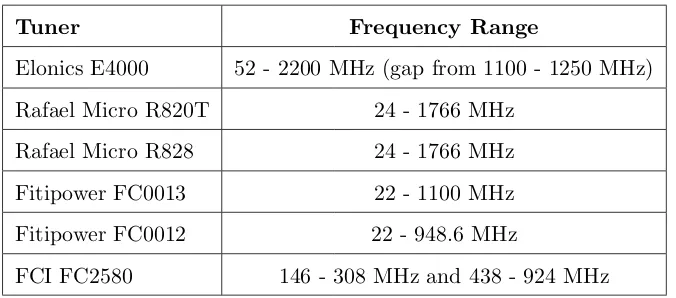
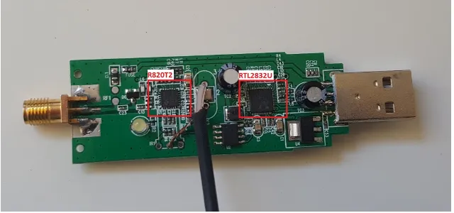
[image:20.595.130.468.512.661.2]

The first stage of an RTL-SDR is the radio frequency tuner. Multiple RF tuners are available on the market, and have been implemented in a wide variety of RTL-SDRs. The following is a summary of the frequency ranges of available RF tuners, provided by osmocomSDR (osmocomSDR, 2015):

Table 3.1: RF tuner frequency ranges (Osmocom 2015).

Tuner Frequency Range

Elonics E4000 52 - 2200 MHz (gap from 1100 - 1250 MHz) Rafael Micro R820T 24 - 1766 MHz

Rafael Micro R828 24 - 1766 MHz Fitipower FC0013 22 - 1100 MHz Fitipower FC0012 22 - 948.6 MHz

FCI FC2580 146 - 308 MHz and 438 - 924 MHz

(21)

[image:21.595.138.458.92.242.2]

3.3 Software 9

Figure 3.1: Location of RF Tuner and Demodulator.

Since the Elonics E4000 is no longer in production, the Rafael Micro R820T is the most popular tuner for RTL-SDR applications. Recently the R820T2 has become available. Kalberla (2015) from the Argelander Institute for Astronomy tested the new R820T2 RF tuner over frequencies between 24MHz 1700Mhz found that the RF820T2 was ap-proximately 2.7dB more sensitive than the R820T, and ran at a 50% reduced system temperature. The R820T2 appears to be the best choice on the market at this current time.

3.2.3 USB Dongle Selection

A USB dongle incorporating both the RTL2832U demodulator and the R820T2 tuner was selected. This dongle can be seen in figure 3.1 containing both components.

3.3

Software

There are numerous software packages available that can process the raw I & Q data received from the RTL-SDR devices. In particular there are two packages that appear to be used most frequently. One is GNU Radio, which is designed to run on a Linux platform. The other is SDR# (pronounced SDR sharp).

(22)

3.4 Signal Sources 10

performed by these blocks are operations such as (but not limited to): filters, channel codes, synchronization elements, equalizers, demodulators, vocoders and decoders.

If the required operation isn’t available as a signal processing block, further functionality can be added through the use of Python script. This results in a very flexible software package that has the potential to be able to deal with any software defined radio operations required. GNU Radio can also be run in simulation mode, if no hardware is connected to the PC. One downside with GNU Radio that has been noted is the difficulty of installing the software. While GNU Radio supports a wide range of RTL-SDRs, there can be some initial difficulty getting the software installed correctly and receiving data from the hardware.

The other popular software package on the market, SDR# by Airspy (AIRSPY 2015), is a windows based software package. This software package is popular, since it is easy to install on a windows platform, and easy to interface with an RTL-SDR USB. SDR# has many basic operations such as spectrum analysis and decoding and playing received audio, but lacks the specific signal processing blocks that GNU Radio uses. Further functionality can be added to SDR# through the installation of third party modular plugins. These plugins can add functionality such a QPSK Demodulator or FFT display. Stringing together functions from these modules can be quite difficult as again, SDR# doesnt have the signal processing block development functionality as GNU Radio, and having modules from different third parties, work together can pose issues.

The software defined radio operations required by this project, will most likely be out of the scope of SDR#. While it may take more time initially to install GNU Radio, the additional functionality will most likely be needed.

3.4

Signal Sources

Multiple potential radio frequencies that could be used for the project were investigated in the literature review. These included phenomena that originated internally and externally to the Earths atmosphere.

(23)

3.4 Signal Sources 11

range, and are created by lighting. Radio waves of this type that are within the audible range (Hz to kHz), and are able to propagate multiple times around the circumference of the Earth’s atmosphere. These particular waves are called whistlers, and can be detected by specialized equipment.

Another source created within the Earth’s atmosphere is that of meteors. The ionization trail (streak of light left by a meteoroid entering the atmosphere), can be detected, as it reflects frequencies between about 30MHz to 150MHz (Entwistle 2014). This is done by using a transmitter to transmit the radio waves at the correct frequency, and a receiver to listen for a reflection.

Sudden Ionospheric Disturbances (SIDs), occur after a solar flare. The radiation from the solar flare swamps the ionosphere, resulting in a very high ionization density with the D region (Gupta, Mitra & Sarkar 1973). A SID can be detected by monitoring VLF transmitting stations. An SID will drastically increase VLF propagation, therefore by detecting an increase in power from a VLF signal, an SID can be inferred, which in turn suggests a solar flare occurrence (Howe 2015).

When detecting radio emissions external to the Earth, there is a certain window of fre-quencies that can be observed. This ranges from 10Mhz at the lower end, due to reflection by the ionosphere (S.Beasley & M.Miller 2008), while the upper limit is about 1.5 THz due to absorption by the lowest rotational bands of molecules that lie within the tropo-sphere (L.Wilson, Rohlfs & Huttemeister 2013). At about 20MHz emissions from Jupiter, at the correct times, can be detected by a two element phased dipole array of about 7m. This is being done as part of a NASA project, called Radio Jove (Nasa 2016) that looks to involve primary, secondary and college students in radio astronomy. Prediction tables give the best times to view these emissions.

Continuum emissions are extra-terrestrial emissions, that are not intermittent and have been mapped extensively over the past century (Wielebinski 2003). It is common for measurements to be taken at the frequency of 408 MHz, and this was done frequently after about 1970, when data processing technology improved.

(24)

precise 1420.405751 MHz. As quoted, in a survey of galactic neutral hydrogen (Kalberla, Burton, Hartmann, Arnal, Bajaja, Morras & Poppel 2005): The emissions from hydrogen are transparent, revealing the whole galaxy better than optical methods. This frequency band 1400 MHz 1420 MHz has been protected by the International Telecommunication Union (ITU), to protect observations of the hydrogen line (Robinson 2001).

Because the nature of this project is to test a noise reducing method, using RTL-SDRs, intermittent phenomenon will not be suitable for testing. This rules out all signals created from sources such as lightning (whistlers) and the detection of SIDs. The testing needs to be replicated as much as possible, therefore continuum emissions will be ideal for use. In particular, the 21cm hydrogen line will be the focus of the project, as it sits at a specific frequency and is well documented.

3.5

Chapter Summary

This chapter investigated and selected appropriate hardware, software and wavelengths to be used for the project. The following has been selected:

Hardware A USB dongle incorporating both the RTL2832U demodulator and the R820T2 tuner has been deemed appropriate for the project.

Software GNU Radio appears to be the ideal software package due to it’s flexibility and ease of writing custom script.

(25)

Chapter 4

Methods of Synchronization and

Radio Astronomy Requirements

4.1

Chapter Overview

This chapter contains the methodology and expected results for each phase of the project. The following topics are discussed: The need for connecting a single clock source to both devices, the measurement of delay between devices, a system for improving the delay between devices, details specifying the construction process of the radio telescopes and measurement methods and principles of radio interferometry.

4.2

Connect Single Clock Source to Both Devices

The R820T2 RF tuner operates on an external 28.8 MHz crystal oscillator. The waveform from the oscillator is passed through a phase locked looped and then mixed with the RF signal to provide an intermediate frequency. This IF is then filtered and fed through to the RTL2832U demodulator. The R820T2 also passes the clock waveform through a buffer and to the external inputs of the RTL2832U. From this it is obvious that both USB devices need to share the same clock signal in order for the outputs to be synchronized.

(26)

4.3 Measuring Delay Between Devices 14

device to the crystal on the other device with a short length of coaxial cable. In effect this will mean that both RF receivers will be receiving clock signals from the same crystal.

To ensure the correct operation after both devices have been connected to a single clock source, the following tests will be carried out:

1. Using an oscilloscope, measure each waveform at the R820T2 and ensure that:

(a) There is no phase difference.

(b) The magnitude of the waveform has not decreased significantly.

2. With both devices connected and powered, test each separately and then together to ensure correct operation and ensure no damage has occurred.

An issue that is likely to occur is that the single oscillator will not be able to provide enough power through the coaxial cable to the other device. This will result in the magnitude of the clock signal on the other device being too low for correct operation. If this occurs the clock signal will need to be passed through a voltage buffer before being received at the other device.

4.3

Measuring Delay Between Devices

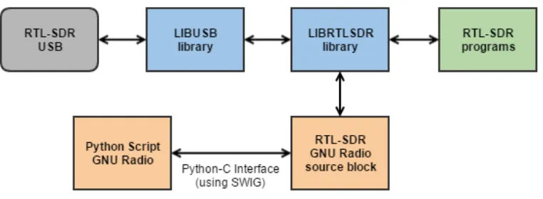
There is a series of software libraries and programs that allow the I&Q signals to be accessed from the demodulator. For the project, the operating system used was Ubuntu 16.04 LTS. The control structure for accessing the I&Q signals is shown in Figure 4.1.

The libusb library contains all the necessary functions to communicate directly with a USB device. The rtl-sdr code base (Osmocom 2015) contains the librtlsdr library that is able to control the operation of the RTL-SDR USB device using the libusb library. There are a few programs that are a part of the rtl-sdr codebase. These programs are able to basic operations with the RTL-SDR USB, although there is are programs that can perform any signal processing operations.

(27)

[image:27.595.104.485.106.246.2]

Figure 4.1: Libraries associated with RTL-SDR USB.

Source blocks provide a stream of data to the system. The data stream from the RTL-SDR USB will be a source.

Sink blocks consume data. These can include graphs and outputs to files.

Functional blocks contain inputs and outputs and are responsible for any signal pro-cessing.

GNU Radio and each block is coded in C. Each block can be linked together with Python script. GNU Radio uses SWIG (Simplified Wrapper and Interface Generator) which gives an interface between GNU Radio and a controlling Python script. The GNU Radio Companion (GRC) provides a graphical interface to further simplify this process.

Both devices will be connected to a single monopole antenna through the use of an RF splitter. The following tests will then be carried out:

1. Through the use of GRC, both sources will be started at the same time as data streams. This data will be placed into binary files. Matlab will be used to compare the delays between both devices over multiple tests.

2. Using the librtlsdr libraries directly, a C program will be written that starts data streams from both RTL-SDR USB devices at the same time. Matlab will be used to compare the delays between both devices over multiple tests.

(28)

4.4 Synchronizing with Switching Hardware 16

at the time.

4.4

Synchronizing with Switching Hardware

This section describes the the use of RF switching and splitting equipment to achieve synchronization between each USB device. In order to carry out radio interferometry the operation of each USB device needs to be synchronized. If both signals were expected to be in phase, a simple correlation of waveforms could be carried out to determine the delay between each device. In the case of radio interferometry it is expected that each device will not receive the same waveform in phase, but rather there will be a slight phase difference depending on the distance between receiving antennas.

An initial idea included the use of an additional antenna for synchronization purposes. Multiple USB devices would all receive the same signal from a single antenna (tuned to a strong signal such as a commercial FM station), the delay between each device would be calculated with correlation and the devices would then be switched back to individual antennas and retuned for the 21cm H-Line. The problem with this method is that every time each device is tuned to a different frequency the delay between each device changes dramatically.

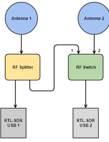
A possible solution to this problem is to use one of the 21cm H-Line antennas as the single antenna to find the delay for both devices. Both devices can receive the signal from the one antenna and after the correlation and delays have been calculated the 2nd, 3rd, 4th... receivers can switch back to their own antennas. This could occur in real time while the each device is running without having to re-tune a device. Figure 4.2 further clarifies the proposed solution:

With reference to Figure 4.2 the following procedure would take place:

1. RF switch is in position 1 and both USB’s are connected to antenna 1

2. Each USB is tuned to 1420.4 MHz and both start streaming data into separate binary files

(29)

[image:29.595.195.383.103.349.2]

4.5 Construction of Antenna Systems 17

Figure 4.2: Proposed method of synchronization.

individual antenna. Note that neither USB will be switched off or re-tuned at this point, so the data stream will be continuous.

4. Both devices will continue running for as long as necessary.

5. This will result in only 1 binary file per device. The 1st second of samples (1st period) from each device will represent the period when the RF switch was in position 1 and the remainder (period 2) will be from when the RF switch was in position 2. The samples from period 1 will be correlated and a delay found. This delay can then be applied to the samples from period 2.

It should be possible to carry out step 5 in real time or during post processing. This proposed solution bypasses the problem of the delay changing every time the devices are retuned.

4.5

Construction of Antenna Systems

(30)

con-4.6 Measurements with Single Antenna and Antenna Array 18

nections will be made with SMA (SubMiniature Version A, 50 Ω) connectors and coaxial cable.

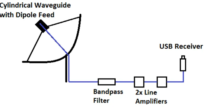
An 80cm dish antenna with a cylindrical waveguide and dipole feed will be used to pick up the required signals. Dish antennas are cheap and widely available for purchase but the waveguide and dipole feed will be manually constructed to save on costs. After the dipole feed, the signal is to be passed through a 1420 MHz bandpass filter and then amplified by two line amplifiers.

[image:30.595.121.473.406.590.2]

Before the second antenna system is constructed the first is to be tested. The methodology of this test is detailed in the next section. The second antenna system will be constructed in the same manner as the first. Once both antenna systems have been constructed and their operation verified they will be integrated together. Instead of connecting directly to a USB receiver, the antenna systems will be connected to the RF switching system shown in figure 4.2.

Figure 4.3: Antenna and Receiving Equipment.

4.6

Measurements with Single Antenna and Antenna Array

(31)

4.6 Measurements with Single Antenna and Antenna Array 19

4.6.1 Single Antenna Measurements

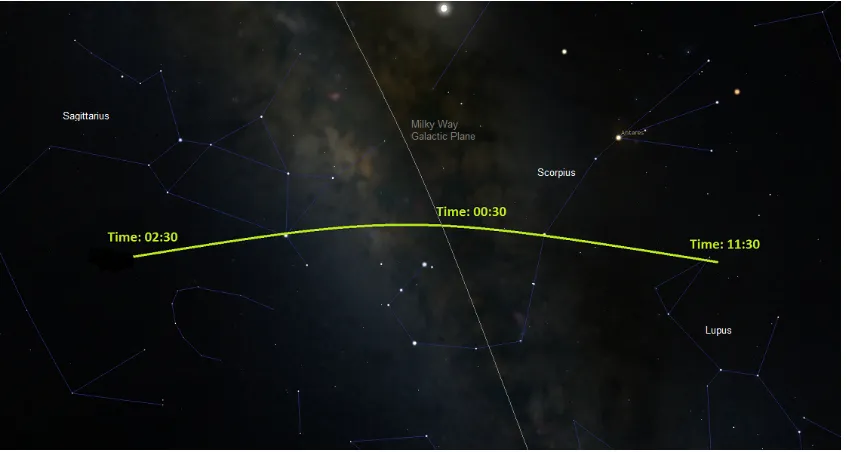
[image:31.595.88.511.238.464.2]

To test the operation of a single antenna the galactic plane of the Milky Way is to be used. Orientating the direction of the antenna to azimuth (90◦), a drift scan is to be carried out that will pass the direction of the antennas over the centre of the Milky Way. To carry out a drift scan, the antenna needs to be simply orientated in one direction and the rotation of the Earth will pass the antenna over a range of locations.

Figure 4.4: Drift scan of the Milky Way. Image generated using Stellarium (2016).

Figure 4.4 shows an example of one of these scans. The time of year is towards the end of May and the time of the scan ranges from 11:30PM to 02:30AM. The scan starts at the edge of the constellation Lupus, passes through Scorpius and the center of the Milky Way and finishes approximately in Sagittarius.

The expected results from a scan such as figure 4.4 is of a signal that drastically increases then decreases in strength as the path of the antenna passes over the center of the Milky Way.

4.6.2 Radio Interferometry

(32)

[image:32.595.114.480.124.391.2]

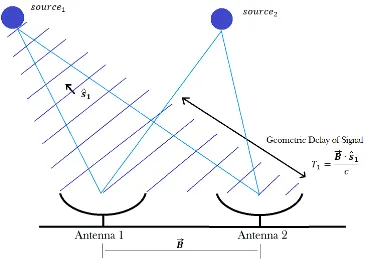
Figure 4.5: Array receiving from two sources.

Vector B~ is the separation between antenna 1 (a) and antenna 2 (b). The unit vector ˆ

s1 is normal to source 1 (S1). T1 is the additional time the signal from S1 takes before

reaching antenna bafter it has already been received by antennaa.

Each antenna will receive the combined voltage from both signals S1 and S2.

The voltage received from both antennas will be:

Ea(t) = e1(t) +e2(t) (4.1)

Eb(t) = e1(t−T1) +e2(t−T2) (4.2)

(33)

f ? g = Z

f(t)g(t−T)dt (4.3)

= Z

[e1(t) +e2(t)][e1(t−T1−T) +e2(t−T2−T)]dt (4.4)

= Z

e1(t)e1(t−T1−T) +e1(t)e2(t−T2−T)...

...+e2(t)e1(t−T1−T) +e2(t)e2(t−T2−T)dt (4.5)

The terms containing bothe1(t) ande2(t) can be removed as the the combination of these

unrelated signals will be noise. This results in:

f ? g = Z

e1(t)e1(t−T1−T) +e2(t)e2(t−T2−T)dt (4.6)

From this equation it can be seen that high cross correlation results will only occur when:

T =−T1 orT =−T2. In these situations the strength of each signal can be found because

the resulting simplified correlation: R

e2₁(t)dt or R

e2₂(t)dt will only contain terms from a single source.

There also may be other sources present which means that there can be strong correlation results for many values ofT.

4.6.3 Antenna Array Measurements

The theory from the previous section can now be applied to the system designed in this project. Each antenna is to be placed apart and the separation between antennas measured. After each antenna has been positioned to point to the same location, the following procedure will occur:

1. Synchronize and start both antennas

2. Cross correlate data from both antennas over entire range of samples. Strong cross correlation results at different values of delay will indicate one or more sources.

(34)

4. Referring to 4.5, the values forc,B~ and eachT are now known. From this informa-tion it is possible to calculate the unit vector ˆsrelated to each source.

5. The cross-correlation result for each source will be R

e2₍_t₎_dt_{, allowing the signal}

strength of each source to be known.

Note that with step four, the precise coordinates of each source will not be able to be determined with only two antennas. Referring to 4.5, the unit vector will only reveal the orientation of the source relative to a two point Cartesian coordinate system (x,y). The plane of this (x,y) system will share points located at each antenna location (a and b) and any point that lie along the direction (altitude) that both antennas are orientated towards. To obtain a three point unit vector, an array of at least three antennas needs to be used so that the exact position of the source can be triangulated.

The angular resolution of a single antenna is:

R= λ

D

whereD is the diameter of the antenna dish andR is the angular resolution. In the case of an antenna array the resolution is:

R = λ

B

(35)

4.7

Chapter Summary

(36)

Chapter 5

Application of Methodology and

Testing

5.1

Chapter Overview

This chapter contains the testing and results for each phase of the project. The follow-ing concepts are implemented are discussed: The connection of a sfollow-ingle clock source to both devices, the measurement of delay between devices, the construction of a system to test for synchronization, the construction and testing of two radio telescopes and finally measurements using the array of two radio telescopes.

5.2

Connect single clock source to both devices

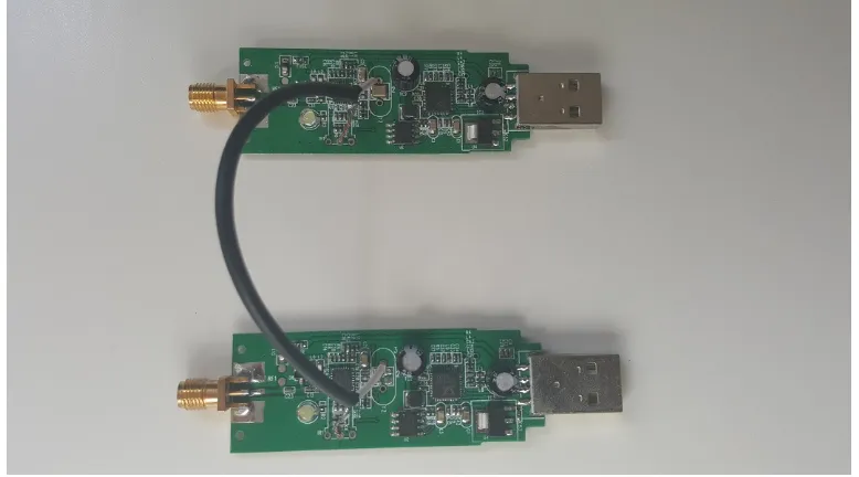
The 28.8 MHz crystal oscillator was removed from one of the RTL-SDR USBs. A short length of coaxial cable was used to connect to connect this device to the crystal oscillator of the other RTL-SDR. The result can be seen in figure 5.1.

(37)

[image:37.595.103.492.145.361.2]

5.2 Connect single clock source to both devices 25

Figure 5.1: Connection of crysal oscillator to both devices.

[image:37.595.87.508.505.711.2]

(38)

Further tests were carried out to ensure the correct operation of each USB device. Both devices were connected to a single monopole antenna through the use of a RF power split-ter. Each device was then simultaneously operated for 5 seconds at a sample rate of 2.4 Mbit/s and the samples stored in separate binary files. Using MATLAB, cross correlation was carried out between sections of samples from each binary file. The samples cross cor-related between each binary file were samples 50e3:150e3, 3050e3:3150e3, 6050e3:6150e3 and 9050e3:9150e3. Using the maximum value of cross correlation the delay was found for each section of samples. In every case this delay was 49572 samples. This demonstrates that the same waveform had been received by each receiver (with a delay) and in turn proves the correct operation of both receivers sharing a single clock source.

5.3

Measuring Delay Between Devices

As per the methodology, two methods were used to used to measure the delay between devices when both have been started simultaneously by software alone.

The rtl-sdr software library contains a program that will tune and start a RTL-SDR device and stream the output I&Q data into a binary file. A C program was written to start this program as a seperate processes for each RTL-SDR device. Memory sharing was used to communicate between the parent and child processes. This script for this program can be found in appendix B section B.1. A dozen seperate tests were carried out, resulting in 24 individual binary files containing the data.

The second method used the GNU Radio environment to perform the same operation. A short python script was created within the GNU Radio Companion environment to run each device for 5 seconds and stream the data into individual binary files, resulting in a total of 24 binary files.

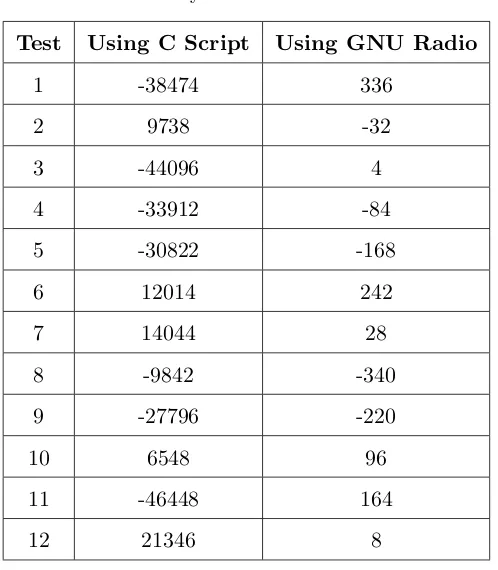
MATLAB was again used to perform cross correlation between samples and find the value of the delay between each device. The results tabulated in table 5.1. The delays present when using GNU Radio range between -340 to 336 samples which is much less than the range of the delays obtained with the C script which range between -46448 to 21356 samples.

(39)

[image:39.595.174.423.110.395.2]

5.4 Test System with Monopole Antennas 27

Table 5.1: Delay between RTL-SDR USB’s.

Test Using C Script Using GNU Radio

1 -38474 336

2 9738 -32

3 -44096 4

4 -33912 -84

5 -30822 -168

6 12014 242

7 14044 28

8 -9842 -340

9 -27796 -220

10 6548 96

11 -46448 164

12 21346 8

restarted the delay varies by a large magnitude. A single value for a delay cannot be found and applied to any further signals.

The poor performance of the C program is due to the fact that it starts multiple copies of a single executive in separate processes. All the overhead of starting individual executives is introduced before data can be extracted from the buffers of each USB device.

5.4

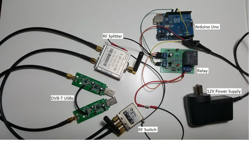
Test System with Monopole Antennas

The system of using a RF switch and power splitter was implemented as described in chapter 4 and figure 4.2. The components for this system can be seen in figure 5.3 and monopole antennas were used for test purposes. The arduino board is being used to control the switching of the RF switch through the relay. A 12 VDC power supply supplies power for both the switch and the relay coil.

(40)

[image:40.595.93.505.92.323.2]

Figure 5.3: Implementation of synchronization system.

signal was located at 953 MHz. During testing of the RF switching system both DVB-T USBs were tuned to that 953 MHz.

The C script already mentioned was modified to control the operation of all the compo-nents for test purposes. Again this script can be found in appendix B section B.1. The script starts both DVB-T USBs and streams the output into separate binary files. Each device is started and controlled by its own process and shared memory controls the timing of each process. Immediately after starting the devices a signal is sent to the arduino that in turn closes the normally open switch on the RF switch for a period of one second. As described in Chapter 4 when this switch is closed both DVB-T USBs are receiving the same signal from a single antenna. After the switch reverts back to its initial position (where each USB device receives a signal from different antennas) the streaming processes continue to run for another 4 seconds.

The binary files created from this processes contain the raw I&Q samples. A MATLAB script is then used to deinterleave this data and correlate the samples at different portions of binary files to test whether the switching system was successful or not. This MATLAB script can be found in appendix B section B.2. The MATLAB script carries out the following operations:

(41)

2. Converts the deinterleaved I&Q samples into magnitude and phase information. In both A and B samples between approximately sample 1 to sample 2.4e6 correspond to the time when both antennas are receiving from a single antenna. Samples from 2.4e6 to 12e6 correspond to its own antenna.

3. Cross correlates samples between A and B that lie between sample 1 and sample 2.4e6. Using this information the script finds the delay between samples.

4. Carries out the same cross correlation between A and B on samples that lie between 2.4e6 to 12e6. Again the scipt finds the delay between samples.

[image:41.595.126.473.450.702.2]

Each monopole antenna was placed no more than 5cm apart. It was expected that the delay from both portions of the samples would be the same and this was confirmed by testing. In over 90% of the tests the delays were 0. In the remaining tests this delay was between 2 and 6 samples. When switching the RF switch, interference can be heard through the computer speakers. This interference may be caused by poor electrical isolation between the relay coil of the RF switch and the contacts of the switch itself. It may be responsible for the 10% of test cases that did not share delays.

Figure 5.4: Correlation of samples between binary files A and B.

(42)

5.5 System Software 30

frequency components are present in each signal.

As noted, the C script is much slower in operation when compared to using GNU Radio. Another consequence of this method is that it becomes very difficult to precisely control the flow of data from each device as each individual process needs to be accessed and controlled by the parent process with shared memory and pipes. This makes it very difficult to processes the data in real time while data is still being streamed from each device.

Using GNU Radio also proved to be problematic. While it was fairly simple to start and stream data from both devices at the same time, it was difficult to control and manage the timing of the RF switch with the timing of the data streams. Controlling individual data buffers also proved difficult. GNU Radio routines are written in C and then accessed through Python with an interface wrapper. While there are almost certainly solutions to control the data and switching with GNU Radio libraries, doing so adds a layer of complexity that is not required with this project.

The solution in the end was to modify the already available RTL-SDR programs. Instead of starting instances of these executables in separate processes, they were modified so only one standalone executable needed to be started that controlled all aspects of switching and data flow. Multiple threads are used within the single executable to manage multiple devices and files. Data flow and control is much simpler with this method as control is much easier accomplished within the same parent process. An explanation of the program is contained in the next section.

5.5

System Software

(43)

5.5.1 Parent Thread

The parent starts both USB receivers and determines all the settings such as frequency and sample rate. After starting each device the delay between devices needs to be calculated before any results can be interpreted. The parent thread will start two instances of a data streaming function in individual threads. These streaming functions will each output a block of data from each device after the devices have been allowed to settle for a few seconds. The parent thread will perform a sliding window correlation between both sets of data and from the results it will calculate the delay present between each device. While this is being calculated, the streaming functions will continue to stream data uninterrupted. After the delay is calculated the parent thread will then start the correlation function in it’s own thread and will then start two instances of the Fast Fourier Transform function in separate threads. The calculated delay is passed into the correlation function as an argument. The parent thread will allow all child threads to run continuously until the user cancels the operation.

5.5.2 Streaming Threads

Two instances of the streaming function are started by the parent thread; one for each device. The streaming function uses a synchronous mode of transfer to transfer data from each device to a data buffer. Each time the synchronous transfer function is called, a block of data of predetermined size will stream from the device to the data buffer. Using this synchronous mode of transfer makes it easier to control exactly how many bytes of data have been transfered so that both streams of data can be maintained in a synchronized manner after the delay has been corrected.

(44)

parent thread. If the stream were to stop or be restarted, the value of delay would be useless as the timing of each device would have changed altogether.

After switching to the functional buffer both streaming threads will continue to run until the user cancels the operation of the entire program. The data in this functional buffer is constantly replaced and discarded as the data is continuously streamed. The function contains a statement that will accept a condition from the correlation thread. When requested each streaming thread will store the contents of the functional buffer in a separate array that will be used by the correlation thread. Notification will sent back to the correlation thread when this transfer of data is complete. This occurs approximately every 250 ms.

Initial versions of the program had the streaming functions continuously sending every byte of data to the FFT and correlation threads for processing. Through testing it was found that the system was only able to perform these calculations approximately 60% of the time before new data was streamed in to each device, resulting in a loss of synchronization and the program crashing. For this reason the FFT and correlation functions will take these small chunks of data only every 250 ms to allow ample time for processing.

5.5.3 Correlation Thread

The function running in this thread accepts the value of delay between devices as an argument. Every 250 ms a notification will be sent to each streaming thread. After the streaming threads have filled a separate array with data, notification will be sent back to the correlation thread. At this point a notification is sent to each FFT thread that data is available for processing. A cross correlation is then performed between both sets of data and the result is displayed on screen.

5.5.4 Fast Fourier Transform Threads

(45)

5.6 Construction of Antennas 33

a FFT. The result is then written to a file that is available to MATLAB for processing. A control file is also written to which signals to the MATLAB script that data is available for processing.

5.5.5 MATLAB

[image:45.595.95.501.314.625.2]

The MATLAB script continuously checks the control file for confirmation that new data is available for processing. Once data is available MATLAB will write this data into its own arrays and display the results of each FFT in real time on two different plots. The plot is updated every 250 ms as new data is received from the system program.

Figure 5.5: Conceptual diagram of system software. Data flow shown by the green arrows.

5.6

Construction of Antennas

(46)

an-5.6 Construction of Antennas 34

tennas constructed using different materials and the last and most successful feed antenna was a cylindrical waveguide with a quarter wavelength probe.

5.6.1 Biquad Antennas

Both biquad antennas were constructed using the same dimensions. These antennas can be seen in figure 5.6 and the dimensions are as follows:

Reflecting plate: Sides of length λ

Length of bowtie: 2λ .

Spacing between reflector and bowtie: λ₈

[image:46.595.104.491.540.747.2]

A signal at 1420.4 MHz was momentarily identified with the aluminium biquad antenna but it not able to be found again and recorded. A poor connection between the reflecting plate and shield of the coaxial cable may be the cause of the poor performance. No signal whatsoever could be identified with the copper biquad antenna. Again it is most likely to be a poor connection between the reflecting plate and the shield of the coaxial cable. A length of half inch copper pipe was used to space the bow-tie element from the reflecting plate. It was very difficult to connect these two components as the the copper pipe is much thicker than the layer of copper on the blank PCB used as a reflecting plate.

(47)

5.6 Construction of Antennas 35

5.6.2 Cylindrical Waveguide and Probe

[image:47.595.122.476.339.575.2]

As already mentioned, a cylindrical waveguide with a quarter wavelength probe was the most successful feed for detecting 21cm hydrogen line emissions. The waveguide can be seen in Figure 5.7. A coffee can that is five inches in diameter was used as the body of the waveguide. The funnel expands the opening from five inches to eight inches and was constructed out of aluminium foil, post card and wire. The penetration for the probe was drilled at an eighth of a wavelength from the back surface of the waveguide. The satellite dish that was purchased came with a mounting arm to locate a LNB (low noise block) down-converter. The mounting arm was cut so the center of the throat of the cylindrical waveguide (at the 5 inch opening) could be positioned in the exact same orientation as the LNB would have been positioned.

Figure 5.7: Cylindrical waveguide with expanded opening.

(48)

[image:48.595.95.500.91.272.2]

5.7 Radio Telescope Measurements 36

Figure 5.8: From left to right: quarter wavelength probe, low noise amplifier, bandpass filter.

5.7

Radio Telescope Measurements

Before constructing the second antenna system and attempting measurements with both antennas, a single antenna was built and tested.

Initially the tests were attempted using GNU Radio on a Linux distribution but there was an issue found when viewing the FFT plot of the received signal. Regardless of the frequency the receiver was tuned to there would be a non-existent signal present on the plot at about -60 dB signal strength. This issue made it very difficult to detect signals under -60 dB as they would not register on the FFT plot. The signal received from the cylindrical waveguide was at approximately -20 dB so it would not have caused any problems in that instance, but when testing the biquad antennas it made it very difficult to know whether they were detecting any signals at all. For this reason SDR Sharp was chosen to perform these initial tests. SDR Sharp gave a simple to use interface that was easy to set up and provided no issues during testing.

(49)

[image:49.595.90.510.204.388.2]

The 21cm hydrogen line sits at a very precise 1420.405751... MHz, but an interesting phenomenon was observed while detecting these signals. Depending on the positioning of the antenna, the frequency could be seen to drift up and down between about 1420.2 MHz and 1420.7 MHz. This may be caused by the Doppler effect and will be investigated further in the following chapter.

Figure 5.9: Signal detected at 1420 MHz.

5.7.2 Double Antenna Measurements

The entire system was set up to be used with the constructed radio telescopes. As a recap the different components used starting from the receiving elements are:

1. Parabolic reflecting dishes

2. Cylindrical Waveguides

3. Quarter wave dipoles

4. Low noise amplifiers

5. Bandpass filters

6. Synchronization switching hardware

7. DVB-T USB Receivers

(50)

[image:50.595.112.485.257.468.2]

This setup of equipment can be seen in Figure 5.10. A bubble level is mounted into the top of the vertical shaft of each mounting tripod. Using this level as well as the markings for elevation on the tripod (from 45 to 90 degrees), both dishes were orientated to point in the same direction at a location close to the center of the Milky Way galaxy. The tests performed and discussed here were taken between the times of 20:30 and 22:30 on the 1st of October 2016 in Londonderry, NSW. Both radio telescopes were orientated to an azimuth of 270 degrees and an altitude of 55 degrees which is an area roughly between the constellations of Sagittarius and Scorpius.

Figure 5.10: Setup of all equipment.

A snapshot of the results are shown in Figure 5.11. As time progressed it was clear that the antennas were not perfectly aligned to the same location. The derivative of the signal strength received by the second radio telescope appeared to lag that of the signal received by the first telescope. The shifts caused by the Doppler effect were very similar on each telescope but it’s still believed they were not perfectly aligned.

(51)

[image:51.595.120.472.99.350.2]

Figure 5.11: FFT results from both radio telescopes.

5.8

Chapter Summary

(52)

Chapter 6

Discussion of Results

6.1

Chapter Overview

This chapter contains discussions of the results of the testing relevant to the main out-comes of the project. Discussed here are: results from the synchronization of both DVB-T USB receivers and the results from the application of this synchronization to radio inter-ferometry.

6.2

Synchronization of Multiple DVB-T USB’s

It was found during testing that the synchronization hardware and software combination was successful in just over 90% of tests. These tests were done by correlating data from sets of around 400 000 samples. No reduction in success rate was obvious until the sample sizes reduced to about 35 000 samples with the success rate at just below 80% for 20 000 sample sizes.

(53)

synchronization and the final controlling program for the entire system. The first step was ensure that the device is allowed to remain off for a few seconds between operation periods of about 60 seconds, and secondly the devices are allowed to run and stream data for a few seconds before synchronization is attempted.

After implementing these changes the success rate improved to 95% over 20 separate tests with the failure only being out of synchronization by 2 samples. The time required to synchronize both devices is not critical when applied to the radio telescope array. Time can also be taken every 60 seconds to reset and resynchronize the devices because the signals being received do not contain modulated data that needs to be interpreted. The synchronization processes takes close to 6 seconds to reset the devices, allow the devices to settle, and correlate the data.

6.3

Application to Multiple Radio Telescopes

While observing the Milky Way with the single radio telescope it was observed that the hydrogen line frequencies varied between approximately 1420.2 MHz and 1420.7 MHz. After investigation it was found that this is almost certainly the result of the Doppler effect. The Milky Way galaxy is in constant motion resulting in the vast majority of objects moving away from the Earth or towards the Earth, resulting in a red shift or blue shift of the received hydrogen line frequencies.

The Dutch Professor Dr. H. van de Hulst (who at the time was an undergraduate student) was the first to make the prediction that neutral hydrogen atoms in the universe would emit emissions corresponding to a wavelength of 21.2 cm (van Loon & Hin 2004). Dr. H. van del Hulst also asserted that because the frequencies were emitted at a known frequency, the Doppler effect could be employed to investigate the velocities inherent in the structure of our galaxy.

(54)

The maximum deviation observed was a red shift of approximately 500 kHz. Using the Doppler effect equation of:

v c =

λshif t−λrest

λrest

This equates to objects moving towards the Earth at a maximum of approximately 100 km/s. It also needs to be noted that the Earth itself is not stationary. The Earth rotates the Sun at an angular velocity of 29.8 km/s which will change the value of red shift or blue shift observed depending on the time of the year.

Expected observed hydrogen line frequencies for the Milky Way Galaxy fall between 1420.0 MHz and 1421.0 MHz (Wilkinson & Kennewell 1994). The frequencies observed fall well within these limits. This is further evidence that the hydrogen line is in fact being observed by the constructed radio telescopes and it is not another signal that may be man made in origins.

6.3.2 Double Antenna Measurements

A major issue related to the sample rate was discovered while investigating methods of radio interferometry. Figure 4.5 gave a basic conceptual diagram of radio interferometry. The geometric delay is the additional distance a signal needs to travel to reach one antenna when compared to the other. After performing a sliding window cross-correlation of the signals received from both antennas, the result is that the peak values of cross-correlation occur at values of delay that correspond in time to the time it takes the signal to transverse the geometric delay. For example if a nanosecond passes between samples and there is a peak cross-correlation results at a delay of two samples, the distance the signal would travel in that time would be:

Geometric Delay = 3×108×2×10−9 = 0.6m

(55)

calculates to be 108 meters. The radio telescopes in this project are separated by no more than 5 meters meaning that the strongest correlation results will always appear at a cross-correlation delay of zero samples. For these reasons it became apparent that radio interferometry was not a suitable application for the DVB-T USB receivers even after they have been synchronized. In the next chapter another use for the synchronized devices is investigated where the sample rate may not be an issue.

6.4

Chapter Summary

(56)

Chapter 7

Conclusion and Further Work

7.1

Conclusion

There were two main objectives associated with this project. The first was to extend the usability of DVB-T USB receivers by providing a method of synchronizing the received signals or producing enough information to correct the delay between devices. The second was to apply these synchronized devices to radio astronomy applications as a proof of concept.

The first objective was successful as both devices were able to be synchronized sample for sample. Connecting both devices to the same clock source ensured that both devices functioned with the same timing. The issue that needed to be overcome was the scheduling of the computer reading the data streams from both USB’s. Each time the receivers were started the delay between the devices would change depending on the scheduling and workload of the computer. This problem was overcome by implementing a hardware switching arrangement that can be used on any system regardless of the operating system.

(57)

7.2 Further Work - Application to Over the Horizon Radar 45

amounts of red-shift and blue-shift depending on the location that was being observed. The level of frequency variation seen within the Milky Way galaxy fit within expected results, which further supported the hypothesis that the signal being observed was indeed the 21cm hydrogen line.

It was identified while attempting to carry out radio interferometry that the sample rate of the receiving devices was a limiting factor to the accuracy of an interferometer in this context. The additional distance a signal will travel between samples is an important factor in determining the accuracy of an array of radio telescopes performing radio in-terferometry. The method designed in this project to synchronize multiple receivers is not dependent on the brand or type of receiver used. As long as received signal can be interpreted in digital form then correlation can be performed in conjunction with the hardware switching arrangement and the devices can be synchronized. If other types of receivers are used with a higher sample rate the accuracy of the system can be improved.

What became obvious throughout the project is the extent of work that can be carried out using cheap and readily available electronics. Software defined radio brings forth a whole field of projects and applications that were once very expensive to accomplish and well outside the range of students, amateurs and hobbyists.

7.2

Further Work - Application to Over the Horizon Radar

The Austrlain Jindalee Over the Horizon Radar Network (JORN) is comprised of three different systems that observe a wide region over Australia’s Northern approaches. These systems are located in Laverton, Alice Springs and Longreach, and have an approximate radar range of 1000-3000km encompassing large sections of Indonesia and Papau New Guinea (RAAF 2015).

Over the horizon radar is capable of ranges that extend beyond the visible horizon. This is achieved by reflecting short wave (3-30 MHz) signals off the bottom edge of the ionosphere to locations at great distance away. If there are observable objects in the path of the signal, the signal will be reflected back a similar path by again reflecting off the ionosphere and arriving eventually at a receiver.

(58)

object of interest but will also comprise components resulting from reflections from the surrounding terrain features such as waves, hills, trees etc... This makes identifiying the reflections of interest amongst all the noise a difficult process. One common method of differentiating these signals is through the use of the Doppler Effect. If an object such as patrol boat is travelling towards the location of the receiver/transmitter equipment the returned signal will have red shifted components that will identify the signal out amongst all the other reflections (Ioana, Amin, Zhang & Ahmad 2010).

For these reasons it is vitally important that the conditions of the ionosphere are known and monitored when operating these radar systems as the ionoshpere is constantly chang-ing with the most noticable differences between day and night. The conditions of the ionosphere are observed through Vertical Incidence Soundings (Ionograms) which involve measuring signals that have been reflected off the ionosphere. Parameters such as height, group delay and electron density can be calculated which allow the precise interpretation of signals received by over the horizon radar systems.

The Australian JORN system utilizes a system of 13 vertical incidence sounders (com-prising of Lowell Digisonde Portable Sounders) in order to produce an updated picture of ionospheric conditions (Harris, Quinn & Pederick 2016). These sounders are set to be replaced in the near future and a few alternatives are currently being tested.

It may be possible that the DVB-T USB receivers investigated in this project can be used in vertical incidence sounding for use with over the horizon radar networks. One of the issues discovered during the project was that the sample rate was a limiting factor when attempting to apply radio interferometry. At a maximum sample rate of about 2.8 MSPS the signal would travel just under 110 metres between samples. When the spacing between radio telescopes is less than 10 metres, the 110 metre geometric delay removes the possibility of accurately calculating position. The Digisonde sounders give a height profile of the ionosphere in increments of 5km (Reinisch 1995). In this case the travel time of 110 metres in between samples may not cause any issues.

(59)

[image:59.595.106.496.92.374.2]

Figure 7.1: Conceptual diagram of vertical incidence sounder.

closest to the transmitting antenna will receive a clear picture of the transmitted signal while the receiver near the receiving antenna will receive the reflected signal. Since both of these transmitted and received signals will be received with a correct time relationship the time of arrival information will be able to be deduced through correlation.

(60)

References

ACT Government (2014), ‘Do a risk assessment’, http://www.worksafe.act.gov.au/ page/view/1039.

AIRSPY (2015), ‘Core tools’, http://airspy.com/download/.

Airspy (2016), ‘R2’,http://airspy.com/airspy-r2/.

Chen, L., Julien, O., Thevenon, P., Serant, D., Pena, A. G. & Kuusiemi, H. (2015), ‘Toa estimation for positioning with dvb-t signals in outdoor static tests’, IEEE Transactions on Broadcasting 61(4), 625–638.

Devendraa Siingh, A. S., Patel, R., Singh, R., Singh, R., Veenadhari, B. & Mukherjee, M. (2008), ‘Thunderstorms, lightning, sprites and magnetospheric whistler-mode radio waves’,Surveys in Geophysics 29(6), 499–551.

Elonics (2010), ‘Multi-standard cmos terrestrial rf tuner’. Pinetown, South Africa.

Entwistle, D. (2014), ‘Radio meteor observing’, http://www.popastro.com/meteor/ observingmeteors/index.php.

Ettus Research (2016), ‘Usrp b210’, https://www.ettus.com/product/details/ UB210-KIT.

Fernandez-Prades, C., Arribas, J. & Closas, P. (2013), Turning a television into a gnss receiver,in ‘Proceedings of ION GNSS+, Tennessee’, CTTC.

GNU Radio (2015), ‘Welcome to gnu radio!’,http://gnuradio.org/redmine/projects/ gnuradio/wiki.

(61)

REFERENCES 49

Gupta, M., Mitra, R. & Sarkar, S. (1973), ‘Some studies on the association of solar optical flares and microwave bursts with sudden ionospheric disturbances’, Journal of Atmospheric and Terrestrial Physics 35(4), 805–813.

Harris, T. J., Quinn, A. D. & Pederick, L. H. (2016), ‘The dst group ionospheric sounder replacement for jorn’,AGU Publications - Radio Science .

Howe, R. (2015), ‘Sudden ionispheric disturbances’, https://www.aavso.org/ solar-sids.

Ioana, C., Amin, M. G., Zhang, Y. D. & Ahmad, F. (2010), ‘Characterization of doppler effects in the context of over-the-horizon-radar’,Radar Conference, IEEE .

Kalberla, Burton, Hartmann, Arnal, Bajaja, Morras & Poppel (2005), ‘The leiden/ar-gentine/bonn (lab) survey of galactic hi. final data release of the combined lds and iar surveys with improved stray-radiation corrections’,Astronomy and Astrophysics

440(2), 775–782.

Kalberla, P. M. (2015), Basic rtl-sdr tests, stability of a new rtl2838u/r820t2 dongle. Argelander-Institut fur Astronomie, Bonn.

L.Wilson, T., Rohlfs, K. & Huttemeister, S. (2013), Tools of Radio Astronomy, sixth edition edn, Springer.

Markgraf, S. (2012), ‘rtl-sdr turns your realtek rtl2832 based dvb dongle into a sdr re-ceiver’.

Nasa (2016), ‘Radio jove’, http://radiojove.gsfc.nasa.gov/.

Osmocom (2015), ‘osmocomsdr’, http://sdr.osmocom.org.

RAAF (2015), ‘Fact sheet - jindalee operational radar network’.

Rafael Micro (2011), ‘R820t high performance low power advanced digital tv silicon tuner datasheet’. Hsinchu County Zhudong, China.

Realtek Semiconductor Corporation (2016), ‘Rtl2832u dvb-t cofdm demodulator + usb

2.0’. http://www.realtek.com.tw/products/productsView.aspx?Langid=1&PFid=35&Level=4&Conn=3&ProdID=257.

(62)

REFERENCES 50

Robinson, B. (2001), Preserving the astronomical sky, in ‘Radio Astronomy and the International Telecommunications Regulations’, Vienna IAU Symposium, pp. 209– 219.

S.Beasley, J. & M.Miller, G. (2008),Modern Electronic Communication, Pearson, Prentice Hall.

Stellarium (2016), http://www.stellarium.org/. Version 0.14.3.

Tseng, S.-M., Change, T.-K. & Hsu, Y.-T. (2012), A/d usb dongle implementation for nb/pc-based software radio dvb-t receiver,in‘The 2012 International Conference on Advanced Technologies for Communications, Hanoi’, IEEE Communications Society, pp. 289–293.

van Loon, B. & Hin, A. (2004), ‘Scanning our past from the netherlands: early galactic radio astronomy at kootwijk and some consequential developments’, Proceedings of the IEEE92(6), 1004–1006.

Wielebinski, R. (2003), The history of radio continuum surveys, in ‘The Magnetized Interstellar Medium’, Max-Planck-Institut fur Radioastronomie, Bonn, Germany.