Development of a baited video technique and spatial models to explain patterns of fish biodiversity in inter-reef waters
143
0
0
Full text
(2) 1.. GENERAL INTRODUCTION. Between coral reefs and on tropical shelves there are vast unmapped mosaics of soft-bottom communities interspersed with shoals, patches and isolates of ‘hard ground’ supporting larger epibenthos. These poorly-known habitats can be dominated by phototrophic corals, seagrasses and algae in clearer waters, and by filter-feeding alcyonarians, gorgonians, sponges, ascidians, and bryozoans in more turbid or deeper waters (Putt et al. 1986; Spalding & Grenfell 1997; Pitcher et al. 2008). The smooth plains and patchy epibenthos support diverse and abundant demersal fish and elasmobranch communities, including large, economically important species, and others comprising ‘bycatch faunas’ (Ramm et al. 1990; McManus 1997; Sainsbury et al. 1997; Hill & Wassenberg 2000; Stobutzki et al. 2001b; Pauly & Chuenpagdee 2003; Ellis et al. 2008; Heupel et al. 2009). Knowledge of fish-habitat associations in these mosaics is generally very poor, principally because of their inaccessibility to SCUBA divers, the taxonomic challenges in identifying the vast diversity of demersal and semi-pelagic fishes found there, and the selectivity of fishing gears used to sample them. Early studies were based solely on trawl surveys associated with commercial fisheries in the tropical Atlantic and Indo-Pacific (Bianchi 1992; Koranteng 2002; Garces et al. 2006a) and were constrained to families of economic interest within the goals of fisheries development or single-species stock assessments. Unlike the demersal fisheries of the temperate zones (Hall & Greenstreet 1998), the diversity and taxonomic uncertainty amongst the vast remainder of the catch has discouraged the maintenance of long-term datasets comparable over large temporal and spatial scales (Pauly et al. 2005). More recently, the need for ‘ecosystem-based fisheries management’ (Sherman et al. 2003; Pikitch et al. 2004) has advanced the identification of difficult families, such as leiognathids, monacanthids and carangids, and has allowed a focus on the range of bycatch species in broad-scale surveys of trawl grounds (Garces et al. 2006b; Stobutzki et al. 2006). The relatively recent concern about overfishing of spawning aggregations of long-lived serranids and lutjanids has also sparked awareness that there exist relatively small, discrete banks and shoals in the ‘off-reef’ habitat mosaics that are critical spawning sites for large piscivores normally associated with fringing and barrier reefs (Coleman et al. 1996; Koenig et al. 1996; Koenig et al. 2000; Scanlon et al. 2003; Mikulas Jr. & Rooker 2008). The depletion by line, trap and spear fishing of these shallower habitats has produced a shift in commercial and recreational effort down-slope or into the ‘inter-reef’ in the ‘Coral Triangle’, the Caribbean, Hawaii and Gulf of Mexico, facilitated by ‘technology leaps’ in marine navigation devices and. 1.
(3) fishing gear that enable small vessels to find and fish these features (Cooke & Cowx 2004; DeMartini et al. 2008). Fisheries managers are not well equipped to deal with this shift in fishing effort in the deep, inter-reef domain because there is almost no information about the distribution and nature of these submerged seabed habitats and their biology (Craik 1989; Pitcher et al. 2002; Salas et al. 2007; Mapstone et al. 2008). The few reviews available suggest that the fish communities on tropical shelves are structured by biogeography, regional sources of upwelling and runoff, thermoclines, mud content of sediments, topographic complexity, depth, latitude, ontogenetic migrations and species replacements through the effects of fishing (Longhurst & Pauly 1987; Lowe-McConnell 1987; Blaber et al. 1994; Sainsbury et al. 1997; Letourneur et al. 1998; Bianchi et al. 2000; Blaber et al. 2000; Bax & Williams 2001; Joanny & Menard 2002; Koranteng 2002; Le Loeuff & Zabi 2002; DeMartini & Friedlander 2004; Parrish & Boland 2004; Auster 2007; Beaman & Harris 2007; Friedlander et al. 2007; Kracker et al. 2008; Anderson et al. 2009). In turn, some species such as serranids and dasyatids may also act as ‘ecosystem engineers’ in modifying the seafloor topography at relatively large scales (Scanlon et al. 2005). Faced with global depletion of fisheries and damage to the ecosystems they inhabit (Myers & Worm 2003; Pauly et al. 2005), the Congress of the United States of America defined the concept of ‘Essential Fish Habitat’ as “those waters and substrate necessary to fish for spawning, breeding, feeding, or growth to maturity” (16 U.S.C. 1802(10). The term ‘waters’ in the definition refers to the “aquatic areas and their associated physical, chemical, and biological properties that are used by fish.” ‘Substrate’ refers to “sediment, hard bottom, structures underlying the waters, and associated biological communities,” and “spawning, breeding, feeding, or growth to maturity” encompasses the full life cycle of the fish (Kelley et al. 2006). To develop an EFH definition for fish species managed under such legislation requires not only an understanding of the influences of substrata and hydrological drivers, but also the other living organisms interacting with that species. As a consequence of this legislation and the desire for ecosystem-based fisheries management there have been some remarkable advances in the application of fishery-independent techniques based on remote sensing of the seafloor topography with laser airborne depth soundings and multi-beam side-scan sonar (Able et al. 1987; Ojeda et al. 2004; Beaman & Harris 2007; Bowell et al. 2008; Wedding et al. 2008), video sensing of seafloor habitats with towed or autonomous underwater vehicles (Pitcher et al. 1999; Holmes et al. 2008; Williams et al. 2009), and direct observations from submersibles (Parker & Ross 1986; Ralston et al. 1986; Yoklavich et al. 2000; Reed et al. 2007). Perhaps nowhere has this been applied more comprehensively 2.
(4) than to the cold-temperate Sebastes rockfish complex (Yoklavich et al. 2000; Anderson et al. 2005; Yoklavich et al. 2007; Love & Yoklavich 2008; Rooper 2008; Anderson et al. 2009; Love et al. 2009), and the Hawaiian banks (Merritt 2005; Kelley et al. 2006). As Stoner et al. (2008) stated, “There is no good substitute for direct observation of fish distribution, behaviour and abundance”, and the development of new ways to make these observations is an imperative of modern marine science. In the case of the Great Barrier Reef Marine Park (GBRMP), only six percent of the total area is comprised of emergent coral reefs and there is a compelling need to provide knowledge of interreef patterns and processes for both their intrinsic value and their relationship with adjacent coral reefs (Pitcher et al. 2000; Pitcher et al. 2007; Pitcher et al. 2008; Coles et al. 2009; Pitcher et al. 2009). Tagging studies are documenting widespread movements between inshore, or offreef, nursery areas and coral reefs for members of a number of economically important fish families (Russell & McDougall 2005; Sheaves 2009), leading to a call for better understanding of this exchange (Sale 2002). There is a rapid diminution in net primary production with depth down the reef slopes, and Polunin (1996) predicted that this is generally accompanied by a down-slope shift toward dominance of larger planktivorous and piscivorous fish. This generalisation remains untested in the deeper (>15m) areas of phototrophic Halimeda bioherms, Halophila seagrass beds and ‘live coral’ habitats in the GBRMP, and on the deep Microdictyon algal meadows of Hawaii (Parrish & Boland 2004). The trophic subsidies provided by filterfeeding megabenthos, such as gorgonians and sponges, are considered to be small (Alongi 1990; 1998), and Hall (2002) proposed that while some juvenile fish do aggregate near seabed structures, our current understanding of the functional role of the larger benthos as habitat features is limited and should be addressed to predict or explain the outcome of chronic disturbances by fishing. The depth limits of scientific SCUBA diving have rendered these fish-habitat interactions very difficult to observe directly. The coarse selectivity and ‘priority effects’ (Whitelaw et al. 1991; Williams & Bax 2001) of the trawls, traps and hook-and-line methods normally used in these depths adds further difficulty in describing patterns of biodiversity (Cappo & Brown 1996), and are prohibited activities for scientists in many areas of the GBRMP. As a result, the patterns and processes in size and species compositions of communities of fishes, so well documented for the shallow reefs of the GBRMP (Williams 1991; Syms & Kingsford 2009), have been poorly studied at depths beyond thirty metres (Watson et al. 1990; Newman et al. 1997; Wassenberg et al. 1997; Burridge et al. 2006).. 3.
(5) In the inter-reef waters of the GBRMP, the managers of fisheries and the marine park require information at the scale of the entire shelf on the vulnerability of metapopulations of inter-reef species to capture by trawling, on the impact of closures to fishing upon biodiversity, and on the ‘comprehensiveness’ and ‘representativeness’ of existing park zoning (Fernandes et al. 2005). This requires fishery-independent survey methods, stratified by knowledge of the key drivers of marine biodiversity as well as spatial position within the shelf. The existence of a long cross-shelf gradient in the central section of the GBRMP has been very well documented for epibenthos, fish and corals along the ‘Townsville transect’ (Williams & Hatcher 1983; Russ 1984; Wilkinson & Cheshire 1988; Gust et al. 2001; Wismer et al. 2009), largely because of the proximity of this section to research institutions and the safety in navigation afforded by the well-mapped, open nature of the outer shelf reef matrix. However, simple application of the cross-shelf models to manage the southern and northern regions are of questionable value because those sections are semi-enclosed by barrier reefs and have much different flushing regimes. It is therefore critical to attempt to provide biologically-informed spatial models of species occurrence to help predict the patterns existing in the GBRMP. These models may have direct application to predicting the fish assemblages on other tropical shelves, or should offer a guide to the selection of key explanatory variables to measure in future studies there. The challenge in providing useful information on inter-reef vertebrates is two-fold. Firstly, nonextractive, non-destructive approaches to surveys of all topographies and zones of the marine park must be developed. Such techniques should have the least selectivity possible, given the fact that a narrow focus in monitoring programs, on economically important predators for example, has great risk of failing to detect fundamental changes in biodiversity (Jones et al. 1993). Secondly, robust models must be developed that explain and predict the distribution of species and assemblages along critical environmental gradients. Relationships between the covariates should be examined for interactions to derive more proximal predictors and surrogates that are easily measured (Williams & Bax 2001; Austin 2007). To overcome the limitations and selectivity of extractive methods, I develop in this thesis a harmless baited video technique that offers the benefits of aggregating fishes of any size by use of bait for visual census on seabed topographies of any form, which is permitted in any zone of the GBRMP. I base this approach on the earlier use of baited video-photography in studies of abyssal scavengers (Priede & Merrett 1996), juvenile lutjanids (Ellis & DeMartini 1995), the fate of bycatch discards (Hill & Wassenberg 2000) and the densities of carnivorous fish inside and outside marine protected areas (Willis & Babcock 2000). Unlike these earlier approaches, I 4.
(6) apply a fleet of up to six replicate units within a ‘biologically-informed’ stratification of the GBRMP study area to describe the spatial patterns of species richness, relative abundance and assemblage structure of demersal and semi-pelagic vertebrates. This was made possible by participating in the largest exploration of seafloor biodiversity ever undertaken on a tropical shelf (Pitcher et al. 2007). Measurements of fish diversity and abundance on even the smooth seafloors of least complexity are notoriously over-dispersed in the tropics. Studies of bycatch faunas show that Indo-Pacific surveys regularly list over three hundred species – yet relatively few species were ubiquitous and these species were not always the ones dominating catches in terms of numbers or biomass (Blaber et al. 1994; Wassenberg et al. 1997; Stobutzki et al. 2001). To further complicate the understanding of spatial patterns, species-environment relationships tend to be inherently asymmetric and non-linear (Austin 2007). They also tend to show heterogeneous scatter of abundances at points along a gradient – often as a consequence of the fact that other unmeasured biotic or abiotic factors are limiting abundances and are interacting with the measured covariates in complex ways (Anderson 2008). To cope with these challenges I chose to use models based on regression trees (De’ath & Fabricius 2000; De’ath 2002; 2007). Boosted regression trees (BRT) and multivariate classification and regression trees (MRT) represent complex information in a visual way that is easily interpretable. They are robust and flexible, because explanatory (predictor) variables can be numeric, categorical, binary, or of any other type, and model outcomes are unaffected by transformations and different scales of measurement of the predictors. They are not sensitive to outliers, and handle missing data in predictors by applying best surrogates with little loss of information. Trees are hierarchical structures, and input variables at the tree ‘leaves’ are dependent on input variables at higher nodes. This allows simple modelling of complex, non-linear interactions that simply cannot be handled by other approaches (Leathwick et al. 2006; Elith et al. 2008). In this thesis I follow key reviews (Longhurst & Pauly 1987; Lowe-McConnell 1987; Longhurst 2007) to derive predictors from the dataset of Pitcher et al. (2007) based on sediment composition, salinity, temperature, depth, seafloor rugosity and epibenthic cover of marine plants and ‘megabenthos’ and infer their relative influence on single species and species assemblages. I also focus on comparing the predictive performance of these environmental covariates with simple measures of spatial position across and along the GBRMP, which undoubtedly act as surrogates for many known and unknown environmental gradients (Fabricius & De’ath 2001; 2008). 5.
(7) My objectives are framed in three main questions, covered in five data chapters: 1.. What are the biases and selectivity in samples caused by time of day, fish behaviour and the use of bait in the application of baited video techniques to describe vertebrate assemblages?. 2.. What are the shelf-scale spatial patterns of species richness and relative abundance in GBRMP inter-reef vertebrate assemblages from 8-80m depths?. 3.. How are these patterns correlated with position on the continental shelf, physical and biological characteristics of the sediments and water column, and epibenthic cover?. These patterns and processes are discussed in reference to the paradigms regarding biodiversity on tropical marine shelves.. 6.
(8) 2.. GENERAL METHODS. 2.1. A REVIEW OF BAITED VIDEO TECHNIQUES TO ESTIMATE RELATIVE ABUNDANCE OF FISH. There has been a recent expansion in the application of baited video techniques (see Table 2.1). In general terms, a bait plume is used to attract vertebrates and invertebrates into the field of view of a video camera where they are identified, counted and often measured. In this brief review I introduce the application of baited video studies using single cameras. The history of the technique may be traced back to searches by Parrish (1989) for the location and nature of key nursery grounds for deepwater Pristipomoides snappers on the Hawaiian shelf with simple camera systems. Meanwhile, the University of Aberdeen’s OceanLab was developing autonomous underwater ‘landers’ with advanced camera systems (e.g. AUDOS and ROBIO) to assess the abundance, behaviour and metabolic rates of demersal scavengers at abyssal depths (Priede et al. 1990; Priede et al. 1994; Priede & Merrett 1996). These systems have video or stills-flash camera units, onboard computer storage of data, and depth, temperature and current sensors. They are retrieved by means of acoustic release of sacrificial weights under buoy packs. Later use of closed-circuit television recording at the surface by Willis & Babcock (2000) sparked further applications to shallow reef sparids and parapercids in studies making comparisons inside and outside marine reserves (Denny et al. 2004; Kleczkowski et al. 2008). Coarse methods of length estimation were used by all of these teams, until the development and testing of stereo-video techniques and software proved that very high accuracy and precision could be obtained efficiently with cheap camera systems (Shortis et al. 2009). The general benefits of the technique lie in three main areas. Firstly, baited video approaches are non-extractive and non-intrusive. This means they can be used in marine reserves, and to gather information on numbers, size and behaviour of animals of special conservation significance. Secondly, large, mobile animals that avoid SCUBA divers and extractive fishing gears are included in samples. This lack of size selection, and the powerful sampling replication afforded by multiple camera units, avoids ‘false negatives’ (Tyre et al. 2003) and allows standardised sampling at any depth, time of day and seabed topography. Thirdly, the acquisition of a permanent tape record removes the need for specialist observers to conduct all fieldwork, allows impartial, repeatable measurements, enables standardised data collection and training in. 7.
(9) association with remote taxonomists (via emailed imagery), and provides a remarkably popular format to communicate science to the public. 2.1.1 General approaches and applications There are two main orientations of bait and camera. Vertical, look-down systems utilise a camera that films a bait canister fixed to a scale bar within a frame on the seabed (Willis & Babcock 2000). This gives a fixed depth of field and a good reference for measurements, but the subjects must be identified by the view of their dorsum from above and the full length of larger animals cannot be seen. Indeed, large sharks and rays cannot physically fit between the camera and the bait. A field comparison by Langlois et al. (2006) showed that major tropical reef fish families, such as serranids, lethrinids and carcharhinids, were shy of entering the field of view underneath a look-down camera. Horizontal, look-outward systems film bait canisters lying on the seabed (Gledhill et al. 2005; Stobart et al. 2007; Wells & Cowan 2007), suspended above the seabed (Merritt 2005), or suspended just below the sea surface to sample pelagic species (Heagney et al. 2007). The depth of field is generally not fixed or measured with such systems, although this parameter can be fixed accurately using stereo-video systems. To identify and count fish all around the bait station, the ‘SEAMAP’ system used by NOAA-NMFS has four cameras filming simultaneously at all points of the compass (Gledhill et al. 2005). The bait plume aggregates fish for counting and measurement through olfactory, auditory and behavioural cues (Armstrong et al. 1992). The action of bait is reviewed in detail in Chapter 3, but in general terms bony fishes, sharks and rays come not just to feed, but are also influenced by the general activity in the field of view. Some species, such as labrids, are highly territorial and, if a video system lands in their home range, they are likely to move about in the field of view in agonistic encounters. Others, like some herbivorous scarids and corallivorous chaetodontids, seem indifferent to the bait, but may be interested in the general activity around it. Fish feeding behaviour at the bait canister stimulates others to approach (Watson et al. 2005) and it is probable that some large predatory carangids and sphyraenids are attracted by the presence of small prey species. Such behaviour has been documented by Whitelaw et al. (1991) for the depredations on captives in fish traps by large serranids.. 8.
(10) Table 2.1. Examples of baited video studies. Abbreviations are HBRUVS/VBRUVS (Horizontal/Vertical baited remote underwater video stations), VBUV /HBUV (Vertical (V) or Horizontal (H) baited underwater closed circuit television), SBRUVS (Stereo horizontal baited remote underwater video stations) and MPA (Marine Protected Areas).. Source. Region. Camera system. Wells et al. 2008. Northern Gulf of Mexico. HBRUVS CCD HandiCams (four camera array). Kleczkowski et al. 2008. Rottnest Island, WA, limestone/algal reefs. VBUV pencil TV camera; VBRUVS CCD HandiCams. Stoner et al. 2008a. Kodiak Island, Alaska, seagrass and algal beds. HBUV low-light monochrome TV camera. Malcolm et al. 2007. Entire NSW coast sub-tropical rocky reefs. Heagney et al. 2007. Lord Howe Island pelagic on shelf to 100m depth. HBRUVS CCD HandiCams. Stobart et al. 2007. Rocky reefs of Spain and France. HBRUVS CCD HandiCams. HBRUVS CCD HandiCams. Depth Range. Diversity (n taxa). Study type. Not reported Lutjanus campechanus. Compare the catch per unit area, length-specific bias, and relative ‘catchability’ (q-ratio) of traps, trawls and cameras for different size classes on low-relief reef habitats.. Not reported 59 spp, 28 fam.. Tests for differences in density, size, biomass and assemblage structure of reef fishes between MPA and adjacent areas using MaxN and length measurements from scale bars.. 2.5-5m. 15-30m. 0+ gadids ; Gadus macrocephalus, Eleginus gracilis, Theragra chalcogramma. Tank tests for reaction to bait; Field tests of Tarr, MaxN and other metrics in comparison with beach seine catches to assess potential for baited video surveys of young-of-the year gadids.. 101 spp, 44 fam.. Tests for effects of along-shelf region (hundreds of kilometres), and within-MPA location (km) scale variation on assemblage structure, and species MaxN. Temporal variation over five years examined in one MPA.. Carangidae (2), Surface Carcharhinidae (2), waters (10m) Scombridae (2), Lutjanidae (1) 10-20m. 51 spp, 31 fam.. Tests for effects of shelf region, MPA zoning, depth, water temperature and current speed on pelagic assemblage structure and abundance (MaxN); Development of simple models to weight results by current speed and plume spread. Comparisons of BRUVS with UVC; examination of species accumulation curves, species arrival times.. 9.
(11) Source. Region. Camera system. Watson et al. 2007. Abrolhos Islands; sub-tropical coral/algal reefs. SBRUVS CCD HandiCams. Cappo et al. 2007a. GBRMP; inter-reef HBRUVS CCD HandiCams and shoals. Langlois et al. 2006. SW lagoon, New Caledonia; coral reef. VBUV CCD HandiCam X 1; HBRUVS CCD HandiCam. RObust BIOdiversity lander Mid-Atlantic ridge (ROBIO) downward facing King et al. 2006 abyssal plain digital stills camera/flash on 1.5 min time lapse. Depth Range. Diversity (n taxa). Study type. 137 spp, 42 fam.. Comparison inside and outside MPAs of ‘target’ and ‘unfished’ reef fish species (species richness, family richness, MaxN).. 8-110m. 347 spp; 58 families of teleosts, chondricthyans and hydrophid seasnakes. Regional-scale community discrimination along spatial and depth gradients.. <10m ?. HBRUVS – 14spp; Serranidae, Lethrinidae, Comparison of remote baited systems (presence/absence Carcharhinidae, Acanthuridae and MaxN). VBUV – 3 spp; Serranidae. 8-12m, 22-26m. 22 taxa; chondrichthyans, holocephalan, teleosts, eels. Including C.(Nematonorus) 924-3,420m coryphaenoides, Synaphobranchus kaupii, Antimora rostrata. Community structure analysis along depth and latitudinal gradients. *Density and length estimates for three species using Priede et al. (1990) models.. Watson et al. 2005. Hamelin Bay; limestone/algal reefs. SBRUVS CCD HandiCams. <10m ?. Gledhill et al. 2005. Gulf of Mexico banks. HBRUVS CCD HandiCams (changing to SBRUVS with low-light, monochrome cameras). 80-120m ?. Lutjanus, Mycteroperca, Balistes. Development of fishery-independent indices of abundance (MaxN, presence/absence), measurement of length, analysis of fish-habitat associations.. Merritt 2005. Hawaiian shelf edge/slope. SBRUVS ultra low-light, monochrome board camera. 200-400m. Pristipomoides, Seriola, Epinephelus. Gear development, fishery-independent indices.. 10. 33 spp; 22 families of teleosts Comparison of diver-swum video and remote baited and and chondrichthyans unbaited video; species richness and MaxN..
(12) Depth Range. Diversity (n taxa). Study type. Tethered VBUV high resolution colour camera. 6-30m. 7 spp, Sparidae, Labridae, Monacanthidae, Pomacentridae, Carangidae, Muraenidae, Scorpidae. Comparisons of MaxN, length measurement inside/outside MPA.. Tethered VBUV high resolution colour camera. ≤50m. Pagrus auratus. temporal comparisons [four years] of MaxN, length measurement.. HBRUVS CCD HandiCams. 1.5-2m. 23 spp; Lethrinidae, Lutjanidae, Haemulidae, Serranidae, Choerodon (Labridae). Comparisons of MaxN inside/outside MPA.. South Georgia/ Falkland Islands. AUDOS downward facing colour film still camera/flash on 1 min time lapse. 900-1,735m. Dissostichus eleginoides, lithodid crabs. Estimates of relative abundance using time of first arrival in Priede and Merrett (1996) model; length estimates.. Hill & Wassenberg 2000. GBRMP; prawn trawl grounds. HBRUVS CCD HandiCam. 10-29m. 9 fish taxa, unidentified sharks, crabs, squid and gastropod. Monitoring fate of discarded fish bycatch at night on the seabed.. Willis et al. 2000. NE New Zealand; sub-tropical rocky/algal reefs. Tethered VBUV high resolution TV camera. <20m. Pagrus auratus, Parapercis colias. Comparisons of time-based indices, lengths, and MaxN inside/outside MPA with angling and underwater visual census (UVC).. 52-87m. Pristipomoides filamentosus, Torquigener florealis. Comparisons of precision, accuracy and efficiency of time-based indices and MaxN from video with longlines; power analysis.. Source. Region. Camera system. Denny & Babcock 2004. NE New Zealand; sub-tropical rocky/algal reefs. Denny et al. 2004. As above. Westera et al. 2003. Ningaloo Reef; coral reef. Yau et al. 2001. Ellis & Hawaii, slopes near HBRUVS CCD HandiCams DeMartini 1995 embayments. 11.
(13) 2.1.2 Estimation of abundance from fish sightings There are a number of measures of the timing and magnitude of sightings of vertebrates that have been derived from tapes to produce counts and indices of abundance. The first type concern the time elapsed before arrival and departure of species in the field of view. The difference between the two times is the duration on tape. The second type comprises the counts of maximum number of individuals (MaxN or npeak) within particular short segments (usually thirty seconds or one minute) or frames of video. Given the nature and expense of field conditions and logistics, it is somewhat surprising that the greatest advances in the theory to estimate densities from these parameters have been made in the studies of abyssal scavengers (Sainte-Marie & Hargrave 1987; Priede et al. 1990; Priede & Merrett 1996). These models do not translate directly to shallow water species, so there has been a marked divergence in indices of abundance between abyssal and shallow studies. These divergent approaches are reviewed here. Very long camera deployments (tens of hours to days) were made to study abyssal scavengers. The foundation of these studies was the theory developed by Priede and Merrett (1996) that the number of fish visible at the bait is the result of an equilibrium between arrivals and departures, and the ‘staying time’ or ‘giving up time’ is governed by Charnov’s marginal value theorem of optimal foraging. This states that the staying time of an animal at an exhaustible food source is inversely related to the probability of finding an alternative food source. Thus Priede et al. (1994) found the npeak of abyssal grenadiers was higher at an oligotrophic location with low fish population and low food abundance because individuals stayed longer at the bait, whereas in a food-rich area with high population density the arrival rate was high because of the higher population, but npeak was low because individuals gave up trying to gain access to the bait and left within an hour. Using strict assumptions that all fish were distributed randomly and evenly, and that they responded immediately, positively and independently from one another to interception of a bait plume, Priede et al. (1990) developed a model of fish density using the ‘shark’s fin curve’. In a plot of number of fish at time t (Nt) against the soak time (t minutes), an initial fish arrival rate is relatively rapid, rising to a peak (npeak) and declining as fish depart. A curve fitted to the data cloud can be broken up into a steeper arrival curve and a shallower departure curve, which are identical in shape, but are separated by a time that corresponds to the mean ‘staying time’ of fish. The difference between the two curves gave the actual number present in the OceanLab studies (Farnsworth et al. 2007).. 12.
(14) Theoretical population densities were calculated by Priede et al. (1990) from the time of arrival of the first scavengers to the bait using an inverse square law: N = C/tarr2 where N is the density of fish per square kilometre, tarr is the time delay between the bait landing on the seafloor and the arrival of the first fish in seconds; C = 0.3848(1/Vf + 1/Vw)2 The constant C depends on the water velocity in (Vw ms-1) dispersing the bait plume downcurrent, and swimming velocity of the fish toward the bait (Vf ms-1). Such estimates are strongly affected by the assumed foraging behaviour of the fish species concerned (Bailey & Priede 2002). Three of the possible foraging strategies (cross-current foraging, sit-and-wait, and passive drifting) of abyssal scavengers produced a distinctive pattern of animal arrivals that may be diagnostic of each foraging strategy. The abyssal scavenger model was tested for Patagonian toothfish by Yau et al. (2001), who noted that for shallow-water applications, the inverse relationship between abundance and the square of the average arrival time will cause problems. Since abundance is proportional to the reciprocal of the square of the arrival time, a doubling of the arrival time produces a four-fold decline in Priede and Merrett’s (1996) abundance estimate. Mean arrival times in shallow deployments occur at the level of seconds to minutes, rather than the tens of minutes to hours recorded in abyssal studies. Shallower deployments also can produce far larger numbers of fish in the field of view. Shallow water studies have therefore neglected a theoretical approach and density estimation in favour of informative comparisons of indices of relative abundance amongst treatments, times and places. Ellis and De Martini (1995) recorded the maximum number seen in a one-second interval (MAXNO), the time of arrival (TFAP), and a total duration of visit during a sequence (TOTTM). Their best video indices of relative abundance were calculated as means to standardise for multiple deployments per station and were derived as: Log of Means (LM) = ln[(ni=1 xi / n ) + 1]. 13.
(15) where xi = the individual datum for a variable (MAXNO, TFAP, or TOTTM) for each deployment at a station, and n = the number of deployments per station. They found that MAXNO for the sharp-tooth snapper Pristipomoides filamentosus and puffers Torquigener florealis was highly correlated with the total duration on video and time to first appearance of the respective species. They also found a positive correlation between MAXNO and long-line catch rates. MAXNO and TFAP were highly correlated, suggesting the greater the snapper and puffer density, the faster the fish arrived at the bait. Willis and Babcock (2000) and Willis et al. (2000) compared the MAXn from baited underwater video (BUV) with underwater visual census (UVC) and angling, and also found that MAXn was positively correlated with fish abundance. Their studies inside and outside a marine reserve included snapper Pagrus auratus and blue cod Parapercis colias. During a thirty-minute BUV deployment, the number of each species recorded at the bait in thirty-second intervals was recorded to derive the MAXsna and MAXcod present in a sequence, together with the time at which the these maxima were recorded (t. MAXsna),. the time of first arrival of each species (t1stsna), and. the persistence of the external bait (tBG). MAXn was the best index, but blue cod responded to bait so well that speed of arrival t1stcod also reflected abundance. Statistically significant effects were detected after only five minutes, and only became more significant with increasing time of deployment of the BUV. The SEAMAP system uses a single ‘pod’, baited with squid, with four cameras mounted orthogonally at a height of 30cm above the seabed (Gledhill et al. 2005). Analysts interrogate twenty minutes of one video tape from each station to identify and enumerate all species. The time when each individual fish enters and leaves the field of view is recorded. This is referred as a time in/time out procedure (TITO). Tapes are sub-sampled if a large number of fish of a given species makes following individual fish difficult, if large numbers of fish occur in pulses periodically during the tape, and if single or multiple schools of fish pass in the field of view. Three estimators of relative abundance are derived from the video data – presence and absence, the maximum count (each individual of each species is counted repeatedly each time it appears in the field of view), and the greatest number of each species that appear at once, termed ‘minimum count’ (mincount). A delta-lognormal model is employed to make a combined annual mincount index from two distinct generalised linear models – a binomial (logistic) model which describes the proportion of positive mincount (presence/absence), and a log-normal model which describes variability in the non-zero mincount data.. 14.
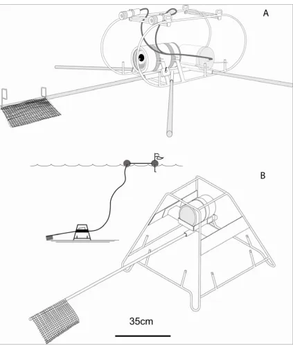
(16) The mincount of Gledhill et al. (2005), the Maxsna of Willis et al. (2000), the MAXNO of Ellis and DeMartini (1995), the npeak of Priede et al. (1996) and the MaxN employed in this thesis are all homologous. They have the advantage of avoiding multiple counts of the separate visits of the same individual fish to the field of view, and they offer conservative comparisons. The laboratory time consumed by tape interrogation and data recording, coupled with observer fatigue, are a major bottleneck in the ‘tape segment’ and ‘TITO’ approaches described above. Tape processing ratios of about 1:1 tape reading time to tape duration were reported for singlespecies interrogation of BUV tapes by T. Willis (pers. comm.) and 13:1 for SEAMAP stations by Gledhill et al. (2005). With the exception of Heagney et al. (2007), shallow water studies are yet to directly estimate the area of attraction caused by bait plumes, but there have been some attempts to ensure that replicates are independent of one another. Ellis and DeMartini (1995) proposed that at distances of greater than one hundred metres separation their replicate ten-minute sets of baited videos were independent, because the greatest distance of fish attraction was only 48-90m for a 200mm fish in a current velocity of 0.1-0.2 ms-1. This assumed a maximum swimming speed of approximately three body lengths per second for a 200mm fish (Vf = 0.6 ms-1). 2.2. BAITED REMOTE UNDERWATER VIDEO STATIONS (BRUVS). The development of the BRUVS hardware progressed from a ‘roll-bar’ frame used in Chapters 3 and 4, to a 700mm high ‘trestle-shaped’ frame that raised the camera housing 480mm above the substratum in the subsequent chapters (Figure 2.1). The higher vantage point was designed to allow a full field of view when vertical cover of gorgonians, plants and octocorals was high, or vertical relief of the seabed was particularly rugose. Frames were fabricated from 10mm steel reinforcing rod and 3mm steel plate and were galvanized. Steel camera arms were bolted onto the trestle frames to provide a camera aspect at an angle of ten degrees to the horizontal (Figure 2.2). To cope with the snagging of BRUVS on hard ground, a system of weak links was designed to enable the legs on the trestle frames to break open and allow the unit to be retrieved (Figure 2.3). Simple camera housings were made from PVC pipe with acrylic front and rear ports (Figure 2.4). Sony™ Hi-8 (model TR516E) or Sony™ Mini-DV HandiCams (models TRV18E, TRV19E) with wide-angle lens adapters (Hama™ 0.5X or Sony™ 0.6X) were used in the housings. The cameras were fixed to a plastic plate and then fitted into the housings through a removable rear port by way of a dove-tail slide (Figure 2.5).. 15.
(17) The cameras were turned on, camera exposure was set to ‘Auto’, focus was set to ‘Infinity/manual’ for the best depth of field and ‘Standard Play’ mode was selected to provide standardised periods of 45, 60 or 90 minutes of filming at the seabed. The cameras were then sealed in the housings before deployment. Flexible bait arms, made from 1500mm lengths of 20mm plastic electrical conduit were attached and detached during and after deployment. The bait arm supported a 350mm plastic mesh bait canister containing one kilogram of crushed oily sardines (Sardinops or Sardinella spp). BRUVS were deployed with 8mm polyethylene or polypropylene ropes and 200-300mm polystyrene surface floats bearing a marker flag, and were retrieved with a hydraulic pot-hauler wheel (Figures 2.1 and 2.7). Ballast weights of 5kg and extra floats were added in conditions where wave action and currents were not mild to prevent the BRUVS toppling and to prevent the head gear being dragged underwater by water pressure on the ropes. The total weight was normally 23kg, but in extreme conditions of swell and current, a fully loaded BRUVS weighed ~43kg at the surface. Once the camera was loaded, the floats and rope were streamed astern of the vessel first, before the BRUVS was lowered into the water (Figure 2.6). A scope of 1½ (shallower than 50m) to 2 (deeper than 50m) times the water depth was used in the length of float ropes. Details of location, time and depth were immediately captured from ships’ instruments using eventlogging software. The vessel approached upwind along the float line to retrieve the BRUVS, and a grapple was cast from the stern quarter to bring the rope aboard and through a snatch block. An hydraulic pot-hauler wheel with variable speed was used to haul the rope, which was manually flaked into a rope bin before being turned over for the next set (Figure 2.7). Replicate BRUVS were set about 300-450 metres apart along transects bracketing sampling stations in this study. This spacing was designed to minimise the possibility of large-scale interference of the replicates with each other. Given a seasonal prevalence of current of ~0.2ms-1 in GBRMP study locations (Vc), the sixty-minute (St) soaks of the BRUVS may have had an effective range of attraction (AR) of ~480m for fish of ~200-300mm length. This comprised forty minutes of advection of the bait plume down-current and twenty minutes of fish swimming time up-current to reach the field of view in time to be recorded on the BRUVS. I formalised this relationship as AR = 60 x (St) x ((Vf x Vc ) – Vc2)/Vf .. 16.
(18) Figure 2.1. BRUVS prototypes used in Chapters 3 and 4 (A) and subsequent chapters (B). For night use, prototype (A) had lights powered by a 12 Volt gel-cell battery enclosed in a housing.. 17.
(19) Figure 2.2. Rubber bonnet tie-downs held housings on camera arm clamps (A, C). Bolting camera arms through slots allowed 10 degrees of tilt (B). A locator lug mated with a socket in the camera housing faceplate (D).. 18.
(20) Figure 2.3. The lug and socket in each leg of the frame (A) used #18 gauge (1.25mm) galvanised wire and a B10 ‘R’ Clip to enable (B,C) or bypass the weak-link (D) .. 19.
(21) Figure 2.4. Rear (A) and front view (B) of a housing showing the fixed, female dove-tail plate for camera, and the lug in the faceplate (B) that fitted a locking pin on the camera arm (Figure 2.2). The locator pin on the dovetail plate (B) locked onto a female lug on the camera baseplate (C). The camera was screwed onto the male plate (C) and slid into and out of the female dove-tail joint with the aid of a wire handle (D).. 20.
(22) Figure 2.5. Loading of camera (A,B) and ballast weights (C,D) to a BRUVS.. 21.
(23) Figure 2.6. Once the camera was loaded (A), the floats and rope were streamed astern of the vessel first (B) , and tied off (C) to await the final position of the drop (D).. Figure 2.7. A grapple was cast to snag the buoy line and bring it through a snatch block for hauling with an hydraulic pot-hauler wheel (A).. 22.
(24) 2.3. PROCEDURES FOR TAPE INTERROGATION. Interrogation of each tape was conducted using a custom interface (BRUVS2.1.mdb©, Ericson and Cappo, unpublished, Australian Institute of Marine Science 2006) to store data from field operations and tape reading, to capture the timing of events and to capture reference images of the seafloor and fish in the field of view. Records were made, for each species, of the time of first sighting, stage (adult or juvenile), time of first feeding at the bait, the maximum number seen together in any one time on the whole tape (MaxN), time at which MaxN occurred, and the intraspecific and interspecific behaviour in eight categories. Species identifications were made according to the Australian CAABCodes national standard (Yearsley et al. 1997) confirmed by checking the collection of reference images with museum taxonomists (Drs B. Hutchins, B. Russell, J. Johnson, and Mr D. Gledhill). It was decided some taxa were indistinguishable on video footage, so these were pooled at the level of taxa, genus, family or order. These taxa, hitherto referred to as species, were signified by the use of ‘sp’ or ‘grp’. The MaxN data were then summed for each species over all single BRUVS replicates at a site. The term ‘fish’ hitherto refers to any marine vertebrate seen in the field of view, including sharks, rays and seasnakes. The tapes were played in a Sony™ DSR20 tape deck with a jog shuttle control to a 50cm screen. The tape deck was connected via ‘firewire’ to the BRUVS2.1mdb, where the video playback was also visible in small windows. The tape was played to and fro and the timecodes (converted to decimal minutes) of important events were captured via firewire from the tape deck. When a new fish was seen, drop-down menus in BRUVS2.1.mdb offered selections for family, genus and species. Once species was selected a CAABCODE was generated with the record. When certain ‘events’ buttons were selected, the timecode was downloaded from the tape deck and stored with the record. The tape deck was paused to allow capture of ‘benthos’ and ‘fish’ images, which were named by the software and distributed to folders. If the species was unknown, various buttons allowed the reference imagery to be searched for a match. If the species was new, a dialogue box enabled generation of custom CAABCodes and a description. The BRUVS2.1mdb added this data to, and called up, ‘operations’ data collected at sea when each BRUVS was deployed. The unique combination of a ‘site’ and a ‘camera number’ linked all records in all tables of the relational database. The database contained information on over 39,900 individual vertebrates seen during the course of fieldwork for this thesis, and over 17,000 images for reference by site, with 2,200 of the best reference images in the ‘reference library’ (Figure 2.8). These protocols, and the design, operation, and troubleshooting for BRUVS2.1.mdb were fully described in a manual. The software and manual can be obtained with the reference image library, under certain terms and conditions of use, by contacting [email protected]. 23.
(25) Figure 2.8. Tape interrogation interface from BRUVS2.1.mdb© (A). Reference image for Pristipomoides multidens, with Lutjanus sebae, L. adetii and Epinephelus undulatostriatus and E. areolatus in the background (B).. 24.
(26) 2.4. STATISTICAL ANALYSES OF INDICES OF RICHNESS AND ABUNDANCE. The MaxN for each species was summed over adults and juveniles within camera replicates, and transformed by 4th root to represent abundance of species i as (∑MaxNi0.25). This transformation down-weighted highly abundant species and reduced skewness in the distributions of values for each species. Species columns were ranked in descending order of prevalence (rather than abundance) in the multivariate data sets, to enable quick filtering of analyses by species occurrence. The number of species was summed to represent species richness (S). A range of other indices were calculated and used in preliminary tests, including indices of taxonomic diversity and distinctness, Pielou’s evenness, Simpson’s index, and the Shannon-Weiner index (Warwick & Clarke 1998; Hall et al. 2006). None of these indices matched simple richness and abundance for ease of interpretation in describing fish assemblages, and they are not presented here. I wished to develop models of univariate and multivariate responses, such as S, ∑MaxNi0.25 and occurrences of multiple species, to detect and describe patterns. To do this I used techniques based on boosted regression trees (BRT) and multivartiate regression trees (MRT). These were introduced to the ecological literature only recently by De’ath (2002; 2007). This approach derives from both classification and regression trees (CART) starting with a data model (De’ath & Fabricius 2000) and from ‘machine learning’ where no data model is specified and algorithms are used to learn the relationship between a predictor and its response (Breiman 2001). Boosted regression trees are therefore an ‘ensemble’ method, whereby models are improved by first fitting many simple models and then combining them for prediction. BRT uses an algorithm from classification CART and a ‘boosting’ algorithm, which combines a collection of models (Elith et al. 2008). Boosted regression trees are complex, but can be summarised in ways that give powerful ecological insight. Detailed descriptions for ecologists with worked examples are available in the papers cited above, and an excellent example of BRT applied to deep water trawl catches is given by Leathwick et al. (2006). Here I provide only a brief summary of those reviews, and the methods are best described in close reference to the presentation and interpretation of results in the following Chapters 5 and 6. 2.4.1 Classification and regression trees (CART) Univariate tree-based models use simple rules to partition the ‘predictor space’ into rectangles to identify ‘regions’ having the most homogeneous responses to predictors. Classification trees fit the most probable ‘class’ as a constant for the region and regression trees fit the mean response 25.
(27) for observations in that region, assuming normally distributed errors. Growing a tree involves recursive binary splits, where a binary split is repeatedly applied to its own output until some criterion for stopping is reached. Predictors and splits are chosen to minimise prediction errors (Elith et al. 2008). Splits are generally chosen to maximise the homogeneity of the resulting two nodes. This is also referred to as ‘minimisation of impurity’ where impurity is defined as the total sum of squared errors of the response variable about the node mean. Impurity takes the value zero when nodes are completely homogeneous. Each binary split minimises the total sum of squares of the response variable within the two nodes, which is equivalent to maximising the between nodes sums of squares (De’ath 2002). Large trees are grown, and then pruned by collapsing the weakest links identified by cross-validation. The terminal nodes, or ‘leaves’ represent the groups of data formed by the tree. Trees can be summarised by their size (number of leaves, or terminal nodes), and by overall fit, or relative error, which is the summed impurity of the leaves divided by the impurity of the undivided, root node (De’ath & Fabricius 2000). The ‘best’ tree has the property of giving the most accurate predictions, on average. The prediction error (PE), or accuracy, of a statistical model is a measure of how close model predictions are to their true values on average. It is dependent on the sum of the bias squared plus the variance and pure error. There is a trade-off between model complexity, bias and variance. Increasing model complexity by adding more parameters decreases bias, but increases variance, and vice-versa. For smaller datasets (n <1,000 cases), like those presented in this thesis, 5-10 fold crossvalidation is used to compare PE in this trade-off. Firstly, the dataset is divided into 5-10 mutually exclusive subsets of approximately equal size (the ‘training’ data). Secondly, each subset in turn is dropped from the analysis, and a tree is grown using data from the remaining subsets. This tree is used to predict the responses for the omitted subset (the ‘test’ data). Thirdly, the estimated error for each subset is calculated. For a sums-of-squares regression tree, the error is the sum of squared differences of the observations and predictions. These errors are summed over all subsets. Fourthly, steps (2) and (3) are repeated for trees of each size. Finally, the tree with the smallest estimated error rate is selected (De’ath 2007). Trees represent complex information in a visual way that is easily interpretable. They are robust and flexible, because explanatory (predictor) variables can be numeric, categorical, binary, or of any other type, and model outcomes are unaffected by transformations and different scales of measurement of the predictors. They are not sensitive to outliers, and handle missing data in predictors by applying best surrogates with little loss of information. Trees are hierarchical structures, and input variables at the tree leaves are dependent on input variables at higher 26.
(28) nodes. This allows simple modelling of complex, non-linear interactions that simply cannot be handled by other approaches (see examples in De’ath 2007). Fitting multiple trees in BRT overcomes the relatively poor predictive power of single trees. The degree to which predictors interact in determining the response can be determined by examining the change in the PE with increasing tree size. For trees comprising a single split, the estimated response depends only on main effects, but trees with two splits include first-order interactions, trees with three splits include up to second-order interactions, and so on. Thus a large increase in the PE from trees of size 2 to size 3, but relatively stable PE for larger trees in the sequence, would indicate strong first-order interactions but no higher-order interactions of importance. The partial dependencies between the response and subsets of different predictors can be quantified to identify precisely which predictors are involved in these interactions (De’ath 2007). 2.4.2 Boosting For regression tree problems, Elith et al. (2008) conceptualised boosting as a form of ‘functional gradient descent’. A ‘loss function’ represents the loss in predictive performance (measured by deviance, for example) due to a suboptimal model. Boosting can then be seen as a numerical optimisation technique that minimises the loss function by adding, at each step, a new tree that ‘steps down the gradient’ of (reduces) the loss function. For BRT, the first regression tree is selected to reduce the loss function to the maximum extent possible for the given tree size. For the second step, the focus is on the residuals of the original tree and the new tree may split on different predictors. After this step the model is updated to contain the two trees as two terms, and the residuals from this two-term model are calculated. A third tree is grown from these residuals, and so on. The process is stage-wise, because existing trees are left unchanged as the model is enlarged. Only the fitted value for each observation is changed at each step to represent the contribution of the newly added tree. This contribution is ‘shrunk’ by a learning rate substantially less than one, because the model-building process performs best if it progresses slowly down the gradient in the loss function. The sequential fitting of trees increasingly focusses on the hardest observations to predict. Thus the final BRT model is a linear combination of thousands of trees that can be thought of as a regression model where each term is a tree. The performance of gradient boosting is also improved by injecting randomness into the sequential fitting (see Friedman 2001; 2002). This involves taking sub-samples of the training data (typically 40-60%) for each iteration (De’ath 2007). This is termed the ‘bag fraction’. It can. 27.
(29) be conceived that if the perfect fit was indeed a single tree, the stochastic gradient boosting process would fit a sum of identical, shrunken versions of this single tree. ‘Regularisation’ of the process is applied to avoid overfitting (Elith et al. 2008). This is done in the relevant ‘R’ libraries by specifying the learning rate as a ‘shrinkage parameter’ determining the contribution that each new tree makes to the growing model, and the tree complexity, or ‘interaction depth’, which controls the interactions amongst the predictors to be fitted. A ‘tree complexity’ of 1 implies a single decision ‘stump’ with two terminal nodes (leaves). This will fit an additive model of only the main effects. An interaction depth of 3 will have two decision nodes and three terminal nodes, and will fit a model with up to three-way interactions, and so on. These two specifications determine the number of trees to be fitted for optimal prediction. A vector specifying the slope of the function relating the response to each predictor can also be used. A parameter of 0 implies the functions can take any shape; 1 implies a monotonic increase; and -1 implies a monotonic decrease. For the value 1 the sign of the slope of the function is always positive (the curve of partial dependence plots tending upwards) or zero (nondecreasing or asymptotic, or depicted as a horizontal, flat line). Likewise, the value -1 constrains the sign of the slope to tend always downwards on partial dependence plots, or be zero. The specification of a distribution for the loss function is foremost in using the boosting technique. For the species richness and transformed abundance data analysed here, the ‘Gaussian’ loss function was used. This function can be used to minimise squared error for continuous outcomes (responses) (Ridgeway 2000; 2007). The ‘Bernoulli’ distribution was used when the responses where classification outcomes, such as presence (1) or absence (0) of a species at a site. For tree-based methods the approximate ‘relative influence’ of a variable is the empirical improvement by splitting on that variable at a particular point (node). Friedman’s (2001) extension to boosted models was to average the relative influence of each variable across all the trees generated by the boosting algorithm. 2.4.2.1 Reporting prediction errors This thesis relied heavily on the reporting of prediction errors. An example is described here to explain the basic implications of these statistics. In the case of analyses of presence or absence of a species at n sites, the data can be envisioned as an n x n matrix of zeroes (absences) and ones (presences). Once the model was fitted, an n x n matrix of predictions was constructed. The two matrices were compared by cross-tabulating the observations with the predictions. Three basic statistics were drawn from the cross-tabulation. The ‘sdt’ was the sum of the diagonals of the table, and it represented the total number of sites for which the predictions were correct. The ‘prediction error’ was the number of sites for which the predictions were incorrect, 28.
(30) which was simply the number of sites, n, minus the sdt (pred.err = n - sdt). The ‘variation in the response explained’ by the model was sdt / n, or (1- rel.pred.err). The ‘relative prediction error’ was the proportion of the overall number of sites for which the predictions were wrong (rel.pred.err = 1 – sdt / n). 2.4.3 Multivariate regression trees (MRT) The BRT approach can be extended by replacing the univariate response by a multivariate response, such as the abundances or occurrence of a large number of species at each site (see De’ath 2002). The impurity measures are redefined as sums of squares about the multivariate mean, which is simply the sum of squared Euclidean distances (SSD) of sites about the node centroid in geometrical terms. Each split minimises the SSD of sites from the centroids of nodes to which they belong. This is equivalent to maximising the SSD between node centroids. Each terminal node (leaf) can be defined by the multivariate mean of its sites, the predictors that define it, the number of sites that grouped there, and by species indicators (see Chapter 2.4.4). A comparison of the MRT with unconstrained, k-means clustering can be used to determine if the tree constrained by predictor variables is accounting for all the groups in the species data. If not, there is some unconstrained variation that is being caused by other variables not included in the analysis. The species that influence the splits most in the tree can be determined in tabular form by partitioning the total species variance by each split of the tree, by the whole tree and by the total for each species (see De’ath 2002). The structure of the multivariate responses can be examined by plotting them in a low-dimensional space using principal components analysis. The ‘distance biplot’ is most appropriate, and species scores projected onto the biplot are located closest to node centroids where they are most abundant. For data characterised by moderate to high alpha diversity, relationships between species dissimilarity and ecological distance can be enhanced by the choice of an appropriate similarity measure and use of extended dissimilarity (De’ath 1999). Dissimilarity matrices were used to grow MRT for some analyses in Chapters 3 and 4. If the dissimilarities are Euclidean distances, a distance-based (db) MRT will be exactly equivalent to the MRT based on SSD (SS-MRT). I used the extended, site standardised Manhattan distance for dbMRT (De’ath 1999). This distance is ‘Euclidean embeddable’, implying that a principal coordinates analysis (PCoA) generates site coordinates where the Euclidean distances between sites are directly proportional to the dissimilarities of sites. Using these coordinates as the responses in an SS-MRT will provide a tree identical to the dbMRT, and in a more efficient manner (De’ath 2002).. 29.
(31) In cases where beta-diversity (species turnover) is high many sites will have no species in common, and ordinations will under-estimate true ecological distance, thereby ‘bending’ such sites toward each other when environmental gradients are portrayed in low-dimensional space. De’ath (1999) developed the extended, site standardised Manhattan distance to overcome this ‘horseshoe effect’, and I used this metric, hitherto referred to as ‘xdiss’, in all distance-based ordinations and MRT in the thesis. 2.4.4 Species indicators for site groups Indicator values (DLI; Dufrêne & Legendre 1997) can be calculated for each species for each node of the trees. For a given species and a given group of sites, the DLI is defined as the product of the mean species abundance occurring in the group divided by the sum of the mean abundances in all other groups (specificity), times the proportion of sites within the group where the species occurs (fidelity), multiplied by 100. The DLI has a maximum value of 100 if the species occurs at all sites in the group and nowhere else. Each species can be associated with the tree node (assemblage) where its maximum DLI value occurred. The index distinguishes between ubiquitous species that dominate many groups in absolute abundance, and species that occur consistently within single groups but have low abundance (Dufrêne & Legendre 1997). This enables use of the numbers of indicator species and their values to characterise each node of the trees. The DLI for species at the root node are simply the prevalence of those species in the entire dataset. Species with high DLI can be used as characteristic representatives of each assemblage, and the spatial extent of the group indicates the region where the species was predominantly found. 2.4.5 Smoothing splines Selected responses and explanatory variables were mapped in two-dimensional space using generalized additive models (gam()). Rather than just treating them as residuals, this approach incorporates non-linearities in the relationship between a response (such as species richness, or measurements of environmental covariates) and the position of the sampling sites ‘across’ and ‘along’ the GBRMP shelf. In simple terms, the gam() used here in Chapters 5 and 6 employed a scatterplot smoother to let the data itself suggest terms representing the non-linearities (Venables & Dichmont 2004). These terms are called ‘smoothing splines’. The flexible gam() does not require the non-linear terms to be parametric or polynomial. The smoothing spline minimises least squares in a ‘penalized’ fashion that controls the trade-off between fidelity to the data cloud and smoothness. I overlaid the colour-contoured plots of the model fits with symbols scaled by the measurements of the response at each BRUVS site. This gave a direct. 30.
(32) visualisation of the smoothed fit in relation to both the original data and the boundaries of the entire GBRMP. 2.4.6 Statistical software All analyses used the open-source ‘R’ statistical package (‘R’ Development Core Team 2006). ‘R’ is a free software environment for statistical computing and data visualisation, maintained on the Comprehensive ‘R’ Archive Network (CRAN). I used the public libraries ‘mvpart’, ‘vegan’, ‘gbm’, ‘car’, ‘MASS’, ‘pixmap’ and ‘maptools’, and another in the Ecology Archives (‘gbmplus’; De’ath 2007)1.. Functions ‘taxondive’ and ‘taxdist’ to calculate (and improve) the Warwick and Clarke (1998) indices of taxonomic diversity and distinctness were developed for my use by Prof. J. Oksanen (University of Oulu) in the package ‘vegan’. Private libraries ‘gdTools’, ‘gbmMV’, ‘veganFuns’, ‘gisTools’, ‘surfer.gam.aa’ ,‘pintol’ and ‘omniRDA’ were provided to me by Dr G. De’ath. These contained powerful functions designed for manipulation, analysis and illustration of data to explore complex interactions of species and communities with their environment, including measures of location and spread for categorical explanatory variables. I used the ‘surfer.gam.aa’ and ‘geoPlot’ functions to carry out the gam() smoothing. These were developed by Dr G. De’ath to analyse ecological data in the low-dimensional space of the position of sampling sites across and along the GBRMP. I overlaid the colour-contoured plots of gam() model fits (prepared with library geoTools) with symbols at each BRUVS site scaled by the measurements of the response. The freely available ImageMagick® software was used for manipulating image formats, and Adobe® Illustrator®was used to polish final illustrations. The bibliography was maintained in EndNote®.. 1. http://www.esapubs.org/Archive/ecol/E088/015/suppl-1.htm. 31.
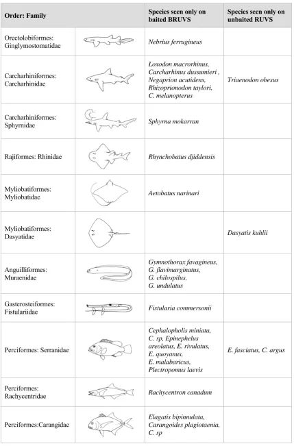
(33) 3.. HOW DOES THE USE OF BAIT AFFECT ABILITY TO DISTINGUISH DEMERSAL FISH ASSEMBLAGES?. 3.1. INTRODUCTION. Critics of the baited video technique persistently argued that there is selection for carnivores and scavengers at the expense of herbivores when bait is used to attract fish into the field of view, yet there were no empirical tests of this presumption in the literature until recently (Watson et al. 2005; Harvey et al. 2007), and it was apparently based on knowledge of the performance of fish traps (see Cappo & Brown (1996) for review). There were indeed striking differences recorded in catches of baited and unbaited fish traps on coral reefs, with a few families of predators (lutjanids, lethrinids and serranids) dominating catches of baited traps, and only herbivorous siganids and scarids predominating in unbaited sets of the same ‘Z’ traps (Newman 1990). However, video footage of the fauna around and outside ‘Z’ traps set in coral reef habitats showed that trap catches were an extremely biased representation of fish diversity regardless of the presence or absence of bait (Cappo & Speare 2004). Baited video recorded higher species richness and abundance than unbaited video in shallow algal reefs (<10m), with significant interactions occurring between sampling location and topographic relief, and sampling technique and topographic relief (Watson et al. 2005). This interaction was caused by higher diversity in the more complex matrix and algal habitat of the high-relief limestone reef. There were numerous species recorded only by the baited video, including larger planktivores and carnivores (Scorpis, Heterodontus, Dasyatis and Seriola). Rarity within the study area did not explain the absence of these genera from unbaited video, because they were sighted on 20-40% of the sites sampled. The same type of comparison was made by Harvey et al. (2007) for both temperate and tropical habitats, but the analyses were aggregated by assigning species to one of ten ‘trophic groups’. Of particular interest was the finding that the use of bait produced slightly more individuals and a higher species diversity of the ‘herbivorous’, ‘invertebrate/algae’ and ‘algae/invertebrate’ feeders. This result contradicted the common inferences about bait attractants made from fish trapping studies. In seagrass, algal reefs and deep sand habitats of the Great Australian Bight, there were significantly higher richness and abundance recorded by baited video for five of the eight trophic groups present. In the lagoon of the GBRMP, and adjacent to emergent and fringing coral reefs, higher mean abundance and richness were recorded when using bait for all tropical functional groups, with the exception of ‘algae/invertebrate’ and ‘sponge/invertebrate’ feeders. Greater numbers of individuals and species were recorded by baited than unbaited. 32.
(34) video in both temperate and tropical marine habitats, and Harvey et al. (2007) considered this to be a major factor in improving the discrimination of these habitat types based on their fish assemblages. The ratio (baited:unbaited) of ‘allocation success’ of a Canonical Analysis of Principal Coordinates (CAP) was 1.15 for temperate habitats and 1.3 for tropical habitats. In this chapter I examine these differences in detail with a more comprehensive dataset, with particular scrutiny of the indicator species and sources of mis-classification of site groups. I compare the performance of video sampling with (BRUVS) and without bait (RUVS) in the deep (>30m) channels between the Palm Islands, and the deep (>40m) lagoon, inter-reef shoals and reef bases of the central GBRMP. My objectives were three-fold. Firstly, I aimed to use linear, univariate models to quantify differences in species richness and abundance. The tests in these models used the presence or absence of bait as a fixed factor, and the location of the sampling as a random factor. Secondly, I used multivariate regression tree (MRT) analyses to distinguish groups in the abundance data at the level of both species and families, and find “indicators” of baited and unbaited video sets. Prevailing criticism of the use of BRUVS concerns bias away from herbivorous groups, so such a bias should be detectable by an examination of the indicators and groupings in the MRT. However, arbitrarily assigning species to trophic groups has proven problematic in the past (see Bellwood 1998), so I used family-level MRT analyses to test if scarids, chaetodontids, siganids and other “non-predatory” families were indicators for unbaited sampling. Finally, an examination of “performance” when comparing techniques (such as baited and unbaited video) should not be limited to comparing metrics such as richness and abundance, or indicator species. Rather, it should test for errors in discriminating and predicting known groups. In this case, I test the success of each technique in discriminating and predicting known groups based on the fish assemblages detected by the MRT. 3.2. METHODS. Six remote underwater video stations of the design shown in Figure 2.1(A) were deployed about 300-450m apart along transects within coarse habitat types in an alternating sequence of baited and unbaited units. The bait canisters on baited units contained one kilogram of crushed pilchards Sardinops neopilchardus. A total of 126 one-hour deployments (sets) of baited (BRUVS) and unbaited (RUVS) units were made in the central section of the GBRMP near Calliope and Curacoa Channels in the Palm Islands, at Robbery Shoals offshore from the Palm Islands, Kelso Shoals, and around Rib and Davies Reefs (Figure 3.1). One hour samples were chosen on the basis of species-sampling time curves derived by Cappo et al. (2001) in the lagoon of a diverse oceanic atoll reef, where most species were sighted within the first 45 minutes of deployment (mean ~ 12.3 ± 6.9), with an addition of less than one species, on. 33.
(35) average, with an increase to 60 minutes soak time (13.5 ± 7.5). Doubling the time on the seabed to 90 minutes accumulated only an extra 3 species (15.3 ± 8.2).. Figure 3.1. Location of video sampling sites in the central GBRMP. Triangle symbols represent baited BRUVS (filled symbols point upwards) and unbaited RUVS (open symbols point downwards).. 3.2.1 Univariate analyses Fish abundances and species richness were univariate responses to the effects of bait and location, and were analysed using univariate statistical approaches (lmer) with the R statistical package (R Development Core Team 2005). The MaxN data were overdispersed and highly skewed by counts made when shoals of pelagic fish passed the field of view, so raw data were analysed with a “quasipoisson” (or “log-link”) function (Ver Hoef & Boveng 2007). The univariate analyses assessed differences in species richness and abundances between the use of. 34.
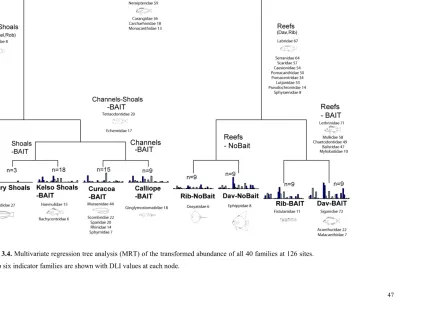
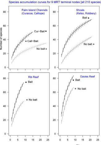
(36) bait (bait) and sampling location (location) using linear, mixed-effects models (lmer) with a quasipoisson link function. This approach can account for unbalanced sampling designs, and does not need prior transformation of raw data. The factor “bait” was fixed and “location” was random. The few samples (3 pairs of baited and unbaited video sets) from Robbery shoals were excluded from the analysis, leaving pairs of samples from Davies and Rib Reefs (each with 9 pairs), Kelso Shoals (18 pairs) and Palm Island Channels (24 pairs). The null model for this design was: response ~ 1+(1|location) where the random effect of location was recognized, but all other main effects and interactions equated to an intercept of 1 The following models were compared with each other and the null model: response ~ bait*location+(1|location) where the interaction of bait and location was recognized, as well as allowing a different intercept for a possible effect of each location response ~ bait+(1|location) where no interaction of bait and location was recognized, but allowance was made for a different intercept for each location. The most parsimonious model was chosen as the one with the lowest Akaike Information Criteria (AIC) in an analysis of variance of the two models. 3.2.2 Multivariate analyses Multivariate regression tree (MRT) analyses were carried out on the entire dataset of transformed species abundances (4th root), including singletons (species seen only once). The data were then amalgamated at the level of family and analysed with MRT. In both cases the DLI (Dufrêne-Legendre Index) were calculated for each node of the trees. Extended, sitestandardised Manhattan dissimilarities (xdiss) of transformed species abundances were used in Constrained Analysis of Principal Coordinates (CAP). This is an ordination method similar to Redundancy Analysis (rda), but it allowed non-Euclidean dissimilarity indices, such as xdiss or Bray-Curtis distance. Function capscale in library vegan was used as a constrained version of Principal Coordinates Analysis (PCoA). This function ordinates the dissimilarity matrix using cmdscale and analyses these results using rda (Oksanen et al. 2009). Permutation tests were made for significant differences in ‘distance variation’ of constrained eigenvalues.. 35.
Figure

+7


Outline
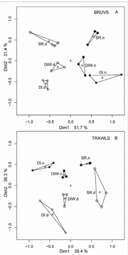
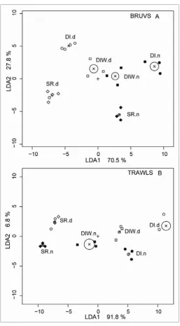
Multivariate analyses
Species richness
Both techniques show selectivity
The role of BRUVS in assessments of seafloor biodiversity
Environmental covariates
Broad-scale spatial patterns in hydrological and sedimentary explanatory variables
The comparative influence of spatial and environmental covariates on species richness
Did a random ‘mid-domain effect’ account for the ‘hotspots’ in species richness?
Broad regional differences in the three sections of the GBR
Related documents