White Rose Research Online [email protected]
Universities of Leeds, Sheffield and York
http://eprints.whiterose.ac.uk/
This is an author produced version of a paper published inGeophysical Journal International
White Rose Research Online URL for this paper:
http://eprints.whiterose.ac.uk/id/eprint/77385
Paper:
Hammond, JOS, Kendall, J-M, Angus, DAC and Wookey, J (2010) Interpreting spatial variations in anisotropy: insights into the Main Ethiopian Rift from SKS waveform modelling. Geophysical Journal International, 181 (3). 1701 - 1712. ISSN 0956-540X
Interpreting spatial variations in anisotropy: Insights into the
Main Ethiopian Rift from SKS waveform modelling
J. O. S. Hammond
1, J-M. Kendall
1, D. Angus
1,2, and J. Wookey
11Department of Earth Sciences, University of Bristol, Wills Memorial Building,
Queens Road, Bristol, BS8 1RJ, UK
2School of Earth and Environment, University of Leeds, Leeds, LS2 9JT, UK
3 March 2010
SUMMARY
1
Seismic anisotropy is a common feature in the upper mantle and measuring shear-wave
split-2
ting in core phases is a common approach in estimating its characteristics. Large lateral
varia-3
tions in estimated splitting parameters are observed over small spatial distances in many
differ-4
ing tectonic regions, including areas of continental break-up such as the Main Ethiopian Rift
5
(MER). We investigate the ability of shear-wave splitting analysis to constrain spatial
varia-6
tions in anisotropy using a one-way wave equation modelling scheme to generate band-limited
7
waveforms for a suite of models representing regions with rapidly changing anisotropy. We
8
show that shear-wave splitting can identify lateral variation in anisotropy on the order of
20-9
50 km, where a change in fast direction demarcates the transition in anisotropy. Additionally,
10
variation in the amount of splitting is complicated close to the transition, and is sensitive to the
11
vertical thickness of anisotropy. We have used these modelling results to interpret shear-wave
12
splitting measurements for the Main Ethiopian Rift. The model that best fits the observations
13
has a 100 km wide rift zone with a fast direction of 30◦ outside and 20◦ inside the rift. The
14
model has 9% anisotropy close to the western margin, with 7% anisotropy elsewhere. In all
15
regions of the model we constrain the anisotropy to begin at a depth of 90 km. The depth of
16
anisotropy is consistent with geochemical estimates of the depth of melt initiation beneath
the region. Also the elevated splitting beneath the western margin supports evidence of low
18
velocities and highly conductive zones from seismic tomography and magneto-tellurics,
sug-19
gesting melt is more focused along the western margin. This study shows how observations of
20
SKS-wave splitting from dense seismic networks can be used to map sharp lateral changes and
21
constrain the depth of the anisotropy.
22
Key words:
23
1 INTRODUCTION
24
Seismic anisotropy can be described as the variation of seismic wave speed with direction of
prop-25
agation. In most studies the main cause of anisotropy in the upper mantle is assumed to be the
26
lattice preferred orientation (LPO) of olivine where the olivine fast axis (a-axis) aligns in the
di-27
rection of upper-mantle flow (Babuska & Cara, 1991; Mainprice et al., 2000). This could be caused
28
by current mantle processes, or due to accumulated strain which has ‘frozen’ in an anisotropic
sig-29
nature from previous deformation events. Other mechanisms that cause upper mantle anisotropy
30
are fluid filled cracks (Crampin & Booth, 1985) or the preferred orientation of inclusions (e.g.,
31
oriented melt pockets (OMP), see Kendall, 1994; Blackman & Kendall, 1997) mechanisms that
32
can be very efficient at generating large amounts of anisotropy (Kendall, 2000).
33
A common way of constraining anisotropy in the upper mantle is shear-wave splitting analysis.
34
When a shear-wave enters an anisotropic medium it splits into two quasi-shear waves that are
35
polarised orthogonally to each other and propagate with different velocities. These split
shear-36
waves can be used to characterise anisotropy in terms of an apparent symmetry axis (typically
37
fast shear-wave direction,φ) and the time-lag between fast and slow shear waves (δt, a proxy for
38
amount, or extent of anisotropy).
39
Many studies investigating upper mantle anisotropy based on shear-wave splitting utiliseSKS
-40
phases. This is a wave that travels as anS-wave through the mantle and aP-wave through the outer
41
core. It is advantageous to use this phase because it is a clear arrival over a range of epicentral
42
distances ( 85◦-120◦), making it observable in most regions. Also, it is possible to ignore source
43
side anisotropy due to the fact that the seismic energy converts to aP-wave at the CMB, thus the
measured anisotropy can be attributed to the mantle beneath the station. Another benefit is that
45
the rays travel almost vertically in the uppermost mantle makingSKS-wave splitting a useful tool
46
to distinguish lateral variations in anisotropy (see Silver, 1996; Savage, 1999; Kendall, 2000, for
47
examples). However, due to the near vertical raypaths it is very hard to place any constraints on the
48
depth extent of anisotropy, which has led to much debate on whether anisotropy can be attributed to
49
lithospheric fabric (fossil anisotropy (Silver, 1996), fluid filled cracks (Crampin & Booth, 1985)),
50
or asthenospheric processes (for example, flow at plate boundaries (Blackman & Kendall, 2002),
51
simple asthenospheric flow (Savage, 1999), density driven flow (Behn et al., 2004)).
52
Some attempt has been made to constrain the depth extent of anisotropy based on consideration
53
ofSKSFresnel zones (Alsina & Snieder, 1995; R¨umpker & Ryberg, 2000). For instance, it can be
54
assumed that two different splitting results from nearby stations indicate that theSKS-waves are
55
sampling different anisotropic regions. Thus, the depth of origin of the anisotropy can be estimated
56
as anywhere shallower than the depth where the Fresnel zones beneath each station overlap. Favier
57
& Chevrot (2003) and Chevrot et al. (2004) apply a finite-frequency Frechet derivative approach
58
and calculate 3-D sensitivity kernels for shear-wave splitting intensity, which are similar to those
59
estimated from Fresnel zone estimates (Alsina & Snieder, 1995; R¨umpker & Ryberg, 2000).
60
Other studies have utilised finite difference modelling schemes to investigate the ability of
61
shear-wave splitting to identify lateral and depth variations in anisotropy (e.g., R¨umpker & Silver,
62
2000), and have placed some constraints on the distribution of anisotropy beneath transform faults
63
and shear zones (R ¨umpker et al., 2003; Chevrot, 2006; Chevrot & Monteiller, 2009) and a
64
plume setting (R¨umpker & Silver, 2000). All these studies show that regions with laterally varying
65
anisotropy give rise to complicated splitting measurements.
66
In this paper we address the suitability of theSKS-wave splitting technique to constrain sharp
67
lateral variations in anisotropy, and further investigate the ability of this seismological technique
68
to constrain the depth extent of the anisotropy. This is done using a finite-frequency waveform
69
modelling technique (Angus et al., 2004). This study improves on previous modeling of laterally
70
varying anisotropy by providing some general guidelines that can be applied to shear-wave
split-71
ting observations in regions with sharp lateral changes in anisotropy. This study was motivated by
observations ofSKS-wave splitting beneath the Main Ethiopian Rift (MER) (Kendall et al., 2005,
73
2006), and these results are used as a case study to highlight the utility of the modeling. This
ap-74
proach is applicable to any region that has sharp boundaries in anisotropy, such as transform faults
75
or suture zones.
76
2 FINITE FREQUENCY WAVEFORM MODELLING
77
We construct synthetic seismograms using the one-way wave equation modelling scheme of Angus
78
et al. (2004) and Angus & Thomson (2006), for waves propagating vertically through a medium
79
containing oriented melt pockets (Figure 2). The model is constructed by calculating the elastic
80
constants for vertically aligned melt pockets, using the approach of Hudson (1981) and applying
81
these elastic constants at each node. The elastic constants are calculated usingP- andS-wave
veloc-82
ities of 7.8 kms−1 and 4.0 kms−1 (matrix material) and 2.5 kms−1 and 0.0 kms−1 (crack material)
83
and densities of 3.8 kg/m3 and 2.7 kg/m3 for the matrix material and crack material, respectively.
84
The cracks consist of penny shaped inclusions with an aspect ratio of 0.01. Crack density is then
85
varied to calculate elastic constants with varying magnitudes of anisotropy. We characterise this
86
anisotropy in terms of maximum shear-wave anisotropy (i.e. 10% anisotropy refers to a maximum
87
shear-wave anisotropy of 10%). Motivated by Kendall et al. (2005) a MER rift-like model is
con-88
structed (Figure 2) (e.g., a rotated horizontal symmetry axis in the rift zone). The simulations are
89
done in 3D, but with only 2D variations in anisotropy.
90
In the models the fast direction is oriented 30◦ from north outside the rift, and north-south
91
inside the rift. AnSKS like wave (i.e. small waveform curvature (4.2−12 s/m), 8 s period) is then
92
propagated through the 3D anisotropic model using the finite-difference one-way wave propagator
93
formulation (Angus et al., 2004; Angus & Thomson, 2006). There is a sharp transition between
94
these two regions (i.e. grid points on either side of the transition between rift and flank have
95
differing fast axis orientations and hence elastic constants). The one-way wave equation method
96
models transmitted waves (it ignores backscattering which is not an issue in modellingSKS-wave
97
arrivals), taking into account frequency dependent coupling effects due to, for instance, rapidly
98
rotating wave polarisation effects due to slowness surfaces (Crampin & Yedlin, 1981).
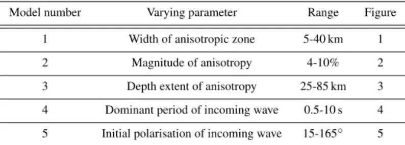
Model number Varying parameter Range Figure 1 Width of anisotropic zone 5-40 km 1 2 Magnitude of anisotropy 4-10% 2 3 Depth extent of anisotropy 25-85 km 3 4 Dominant period of incoming wave 0.5-10 s 4 5 Initial polarisation of incoming wave 15-165◦ 5 Table 1.Parameters tested in the various models
All waves are Ricker wavelets (although wavelet type has no effect on the result), have a
100
dominant period of 8 s (except model 6, where frequency dependence is investigated), and initial
101
source polarisation of 45◦(except model 7, where initial polarisation dependence is investigated).
102
The output waveforms are then analysed identically to the data (see Kendall et al., 2005), and the
103
apparent splitting is estimated for a profile spanning the ‘rift’ zone.To estimate the splitting we
104
use the Teanby et al. (2004) cluster analysis method which is based on the Silver & Chan
105
(1991) method. This technique performs a grid search overδt andφ, rotating the horizontal
106
components by φ, and shifting their relative positions by δt. The values of δt and φ which
107
provide the most linear particle motion provides our estimate of the splitting. A statistical
108
F-test is used to asses the uniqueness of the result, thus providing an error estimate.The
ob-109
served splitting depends on several parameters (outlined in Table 1) and each parameter is studied
110
in turn (Figures 3-7). Finally, based on the modelling results, the observed splitting parameters of
111
Kendall et al. (2005) (Figure 1) are modelled to place estimates on the anisotropic characteristics
112
beneath the MER.
113
2.1 Model class 1: Varying width of ‘rift’ zone
114
The first variable tested is rift width (all other variables are held constant: maximum S-wave
115
anisotropy=10%, depth of anisotropy=45 km (from surface), dominant period=8 s, initial polarisation=45◦).
116
We vary the width of the rift zone between 100 km and10 km(Figure 3). A smooth transition in
117
φ is seen for all rift widths. The inflexion point in the φ profile marks the boundary between
118
anisotropic regions (Figure 3). However, δt shows considerably more variation across the rift
119
boundaries. The expected δt for this model is a constant value of 1.27 s, but we see large
ations, similar to those seen for other studies of inhomogeneous anisotropic media (e.g., plume,
121
R¨umpker & Silver (2000); transform fault, R¨umpker et al. (2003)).
122
2.2 Model class 2: Varying magnitude of anisotropy
123
The second variable tested is the magnitude of anisotropy (all other parameters are held
con-124
stant: rift width=40 km, depth of anisotropy=45 km (from surface), dominant period=8 s, initial
125
polarisation=45◦). All models within this class show a smooth transition inφ, with the inflexion
126
point showing the transition between anisotropic regions. Theδt profile shows a similar trend for
127
all models. The magnitude of splitting depends on the amount of anisotropy, but the peaks and
128
troughs of theδt curve all lie in the same place (see Figure 4).
129
2.3 Model class 3: Varying thickness of anisotropic zone
130
The third variable tested is depth (i.e. thickness from the surface) of the anisotropic zone (all other
131
parameters are held constant: rift width=40 km, maximumS-wave anisotropy=10%, dominant
pe-132
riod=8 s, initial polarisation=45◦). The variation ofφis smooth for nearly all models in this class,
133
with the inflexion point showing the transition between anisotropic regions. An exception occurs
134
in the model with an 85 km thick layer (Figure 5). The variation inφseen in the 85 km thick layer
135
has some deviation at the boundary between anisotropic regions. This may be due to multipathing
136
effects; a result of the longer wavepath through a complex, highly anisotropic medium. The δt
137
curve shows similar variation to that seen in model 2. Although similar to model 2, where the
138
magnitude of splitting increases with anisotropic strength rather than increasing path length, there
139
is an observable moveout of the peaks with increasing thickness (Figure 5). This sensitivity with
140
depth can be used to interpret something about the depth to the anisotropic region. We discuss this
141
further in relation to the MER results in section 3.1.
142
2.4 Model class 4: Varying frequency of propagating wave
143
The fourth variable tested is the dominant period of the incoming wave (all other parameters are
144
held constant: rift width=40 km, maximumS-wave anisotropy=10%, depth of anisotropy=45 km,
initial polarisation=45◦). It is evident that varying the dominant period has a large effect on the
146
variation observed in bothδt andφ(Figure 6). For higher frequencies the curves match the input
147
model well, with little deviation inδt and a sharp transition inφ. The observation that the inflexion
148
points in φ describe the width of the rift zone still applies for all frequencies. For higher
fre-149
quencies the peaks inδt are narrow, an effect of approaching the ray theoretical limit. This shows
150
the importance of investigating shear-wave splitting using a finite-frequency approach, where the
151
influence of frequency dependent shear-wave coupling is accounted for.
152
2.5 Model class 5: Varying initial polarisation of the incoming shear wave
153
The fifth variable tested is the initial polarisation of the incoming wave (all other parameters are
154
held constant: rift width=40 km, maximumS-wave anisotropy=10%, depth of anisotropy=45 km,
155
dominant period=8 s). The variation inφis dependent on the initial polarisation, but the inflexion
156
points still define the width of the rift zone (Figure 7). The transition inφ from 30◦ to 0◦ occurs
157
over distances of∼20-50 km. It is evident thatδt is strongly dependent on the initial polarisation,
158
with the peaks inδt occurring either side, and on top of the transition between anisotropic regions
159
(Figure 7). This is similar to previous studies of inhomogeneous anisotropic structure which show
160
that the measured splitting parameters are highly dependent on the initial polarisation of the
shear-161
wave (Silver & Savage, 1994; R¨umpker & Silver, 2000; R¨umpker et al., 2003).
162
The variation in theδt profile depends on the relationship between the initial polarisation and
163
the two anisotropic symmetry axes. For example, model 5 shows that for an initial polarisation
164
of 105◦ the peak in theδt curve lies directly above the transition zone. This initial polarisation is
165
oriented 75◦ from both the 30◦ fast direction outside the rift, and the 0◦ inside the rift (105◦ =
-166
75◦).However, when the initial polarisation is preferentially close to one of the symmetry axis
167
(assuming it is not so close that a null measurement is recorded), it will induce an asymmetry
168
in the observedδt measurements. This result is consistent with the observation that the
finite-169
frequency sensitivity kernel of the incoming shear-wave depends on the initial polarisation (Favier
170
& Chevrot, 2003; Chevrot et al., 2004).”
3 DISCUSSION
172
For all the scenarios modelled in section 2 it is evident that sharp lateral changes in anisotropic
173
fabric can be detected using shear-wave splitting. The sharpness of the transition in splitting
pa-174
rameters depends on three parameters, the thickness of the anisotropic layer (Figure 5), the
fre-175
quency of the incoming wave (Figure 6) and the initial polarisation of the shear-wave (Figure 7).
176
For example, for an 8 s wave (e.g.,SKS), the transition inφ from 30◦ to 0◦ occurs over ∼20 km
177
(25 km thick layer) to∼40 km (85 km thick layer), assuming a constant initial polarisation. For a
178
constant thickness of anisotropy (45 km) the transition inφvaries from∼20-50 km, depending on
179
the initial polarisation. In all model classes, except where the splitting is very large, the inflexion
180
points in theφcurve define the transition in anisotropic fabric. For the MER this will indicate the
181
rift width, but this phenomenon can also potentially be used to determine the location of transform
182
faults and suture zones.
183
Having constrained the rift width fromφ it is possible to use the variation inδt to place
con-184
straints on the thickness of the anisotropic layer. The position of the peaks and troughs inδt vary
185
for differing rift widths, frequency content of the incoming wave, thickness of the anisotropic
186
layer and initial polarisation. By assuming a dominant period of the incomingSKS-phase of 8 s,
187
we can use the position of the peaks and troughs to estimate the thickness of the anisotropic layer.
188
This can only be done for one initial polarisation (approximately the same as back-azimuth for an
189
SKS-wave).
190
From studying the variations inφandδt we can estimate the width and thickness of the
anoma-191
lous anisotropic zone, and from this it is simple to estimate the magnitude of anisotropy. The
mag-192
nitude of anisotropy is calculated by determining the amount needed to match the splitting results
193
far from the rift. In our models we impose a vertical transition in anisotropic regions. We
acknowl-194
edge that dipping boundaries may effect these results, and more modeling is need to constrain
195
this.
196
This modeling exercise has highlighted other features which may be observable in data to
de-197
tect lateral variations in anisotropy. It is evident that stations close to the transition will show large
198
variation inδt as a function of back-azimuth, whereas the same stations will show little variation
ofφ. This is notably different from what is expected from two horizontal layers of splitting, which
200
causes variations in bothφandδt (Silver & Savage, 1994). Another feature which can be observed
201
is the variation ofδt as a function of frequency, again close to the transition in anisotropic domains.
202
3.1 Comparison with the Main Ethiopian Rift (MER)
203
Kendall et al. (2005) observe a rotation in the splitting fast direction inside the Main Ethiopian
204
rift valley, with the fast shear-wave aligning with the magmatic segments (Figure 1). This pattern
205
could be caused by oriented melt pockets (OMP) or along-rift flow which causes a lattice preferred
206
orientation (LPO) of olivine. A study of surface waves (Kendall et al., 2006; Bastow et al., in
207
review 2010) addresses this ambiguity, due to the azimuthal variations expected for observed
208
phase velocities on interstation paths being different for OMP or LPO.Kendall et al. (2006) and
209
Bastow et al. (in review 2010)show that to satisfy both theSKS-wave splitting results and surface
210
wave results an OMP source of anisotropy, down to depths of at least 70 km, must be present. Keir
211
et al. (2005) analysed splitting in shear-waves from local earthquakes<20 km beneath the MER,
212
and found fast directions similar to Kendall et al. (2005), aligning with the magmatic segments.
213
They also found elevated splitting magnitudes above regions where melt has been inferred from
214
wide-angle refraction (Mackenzie et al., 2005) and controlled source tomography (Keranen et al.,
215
2004).
216
Other SKS-wave splitting results around Ethiopia show similar results. Ayele et al. (2004)
217
observed splitting in Kenya, Ethiopia and Djibouti, and noticed that the magnitude of splitting
218
increases with the amount of melt produced, inferred from a correlation between an increase in
219
delay time and volcanism. Gashawbeza et al. (2004) performed shear-wave splitting on a network
220
of wider aperture, but similar location to Kendall et al. (2005). They observed similar rift parallel
221
trends in the fast directions, but argued that fossilised Precambrian anisotropy was the source of
222
this splitting, with some more recent Neogene influence near the rift to explain the rotation in the
223
fast directions.
224
Melt has been observed beneath the plateau in the form of highly conductive bodies in
magneto-225
telluric surveys (Whaler & Hautot, 2006), and underplating is observed in wide-angle reflection
profiles (Mackenzie et al., 2005). It seems likely that a combination of both pre-existing fabric,
227
and melt induced anisotropy could be present beneath the plateau region. Further evidence of melt
228
beneath the MER comes from receiver function studies. High values of Poisson’s ratio>0.3 for the
229
average crust, and underplating highlight the likelihood of melt beneath Afar (Dugda & Nyblade,
230
2006) and the MER (Stuart et al., 2006).
231
Using the criteria outlined in the previous section we can match the pattern of results observed
232
by Kendall et al. (2005) (Figure 1), and thus place more constraints on melt induced anisotropy
233
beneath the MER .
234
As was shown in the previous section, the variation of φ is relatively insensitive to all
pa-235
rameters (assuming an instantaneous change in anisotropic parameters at the transition), and the
236
observation that the ‘rift’ width can be defined by the inflexion points is robust, except in the
pres-237
ence of very high splitting. For the EAGLE dataset, this results in a rift width of∼100 km, based
238
on all the splitting results from different back-azimuths, with a fast direction of 30◦ outside the
239
rift, and 20◦ inside the rift (Figure 9).
240
We have shown that variation inδt is dependent on frequency, initial polarisation and vertical
241
thickness of the anisotropic zone.To model this event we take a real SKS waveform from the
242
Ethiopian seismic station ADEE (Figure 8) (see Bastow et al., 2008, for station details), and
243
propagate this through the model . However, an 8 s Ricker wavelet, as used in the previous
244
sections, produces identical results. We can not use all the data, as we did for measuring the
245
rift width, as they come from differing back-azimuths. To account for this we take results from
246
one very well constrained SKS-wave splitting event that was recorded across the whole array.
247
This event has a back-azimuth of 40◦. We run a model, based on this information, to estimate the
248
depth of the anisotropy. The model has a 100 km wide rift zone, 10% anisotropy, a fast direction
249
of 30◦ outside the rift and 20◦ inside, an initial polarisation of 40◦ and a period of 8 s (Figure
250
10). It is evident that the peaks are moving out with anisotropic thickness, and if we plot the
251
peak-peak width as a function of depth it is evident that they lie on a straight line (Figure 10).
252
This observation is valid for initial polarisations which fall outside the null planes of either of the
253
anisotropic regions, and outside the null planes for effective splitting parameters observed near the
transition between anisotropic regions. For the event with back-azimuth of 40◦the peak-peak width
255
is 133 km (Figure 9), which equates to a depth of 90 km. With this information we can estimate
256
the magnitude of anisotropy needed to generate the amount of splitting observed. However, the
257
peaks seen inδt vary in magnitude with the western plateau having elevated shear-wave splitting
258
compared to the eastern plateau. As a result we propose a model which has 9% anisotropy on the
259
western plateau and in the westernmost 30 km of the rift zone and 7% anisotropy on the eastern
260
plateau and easternmost 70 km of the rift zone (Figure 9). Unfortunately, no other events were
261
suitably recorded across the whole array and thus comparisons of this model with splitting
262
results from other back-azimuths can not be performed..
263
We estimate a region of anisotropy which extends to a depth of∼90 km beneath the MER,
ex-264
tending beneath the two margins and the rift valley. On the margins the anisotropy is oriented with
265
a fast direction of 30◦, and beneath the rift valley the anisotropy is perturbed with an orientation of
266
20◦. The anisotropy below the rift valley correlates with the magmatic segments, as described by
267
Kendall et al. (2005). The variation evident inδt can largely be explained as an effect of these two
268
different anisotropic regimes interacting. The variation inδt is highest on the western margin and
269
results in an estimate of 9% anisotropy beneath this region compared to 7% on the eastern margin.
270
This model is summarised in Figure 11.This model was estimated using a trial and error
ap-271
proach. To fully constrain this model requires a more complete sampling of the whole model
272
space, which is computationally impractical. As a result we can not formally discuss errors
273
of the fit to the data here. To provide confidence in our models we can compare our results
274
with other geophysical data. To fully explore the model space, studies that invoke theoretical
275
sensitivity kernels may be suitable (Chevrot, 2006; Chevrot & Monteiller, 2009).
276
If anisotropy is derived from oriented melt pockets, as suggested by Kendall et al. (2005) then
277
this suggests that melt present beneath the MER is aligned from a depth of 90 km, with an average
278
anisotropy of 7-9%. This equates to a melt fraction of 7-9%, assuming vertically oriented isolated
279
melt inclusions with an aspect ratio of 0.01, but the amount of melt needed to produce this amount
280
of splitting would be smaller for inclusions with a lower aspect ratio.
281
This estimate of the depth extent of melt induced anisotropy is supported by other studies.
Kendall et al. (2006) show that azimuthal anisotropy seen in surface wave results occurs at depths
283
between 50-70 km, and may extend further but resolution decreases below these depths. Based
284
on simple Fresnel zone estimates, Kendall et al. (2005) place the origin of the anisotropy seen
285
in the EAGLE data to be <100 km, a fairly accurate estimate based on these results. P- and S
-286
wave tomography show the lowest seismic velocities in the top 100 km (Bastow et al., 2005, 2008)
287
(Figure 11) and Ayele et al. (2004) image a discontinuity at a depth of∼90 km which they suggest
288
is the base of the lithosphere. Based on geochemical evidence, Rooney et al. (2005) suggest that
289
the base of the lithosphere is the origin of melt generation feeding the MER. Additionally, Keir
290
et al. (2009) suggest that partial melting of the lithosphere and subsequent magma injection causes
291
lower crustal earthquakes throughout the MER and western plateau.
292
Seismic tomography (Bastow et al., 2005, 2008) (Figure 11) and magneto-tellurics (Whaler &
293
Hautot, 2006) both show evidence for an asymmetry in melt production, with lower velocities and
294
higher conductivities present beneath the western plateau compared to the eastern plateau. This
295
is supported by our results which show elevated anisotropy in the west, mainly at the region we
296
define as the rift boundary. Holtzman & Kendall (in review) suggest that melt is concentrated in
297
regions of higher strain, and cite the elevatedδt seen by Kendall et al. (2005) as evidence for this.
298
We show that an elevatedδt can be explained by a simple variation in fast direction alone across
299
the region, but we still require elevated anisotropy close to the western margin, as suggested by
300
Holtzman & Kendall (in review), to explain the asymmetry seen inδt.
301
4 CONCLUSIONS
302
We have developed a modelling technique, using a one-way wave equation approach, to investigate
303
the effects of laterally varying anisotropy on shear-wave splitting. We have shown that:
304
(i) SKS-wave splitting can be used to identify changes in fast direction over lateral distances of
305
20-50 km (dependent on depth and initial polarisation).
306
(ii) The inflexion points in theφprofile demarcate the transition in anisotropy.
(iii) Variation in the position of the peaks and troughs seen inδt depend on anisotropic thickness
308
from the surface, and for a given initial polarisation can be used to place depth constraints on the
309
anisotropic region.
310
(iv) With information on the depth of the anisotropic region, estimates can be placed on the
311
percentage of anisotropy in the region.
312
(v) At stations close to the transition δt varies as a function of back-azimuth and frequency,
313
whereas φ shows little such variation. This can be used as an indicator of lateral changes in
314
anisotropy
315
(vi) For higher frequencies the modelled splitting approaches the ray theoretical limit, and
316
shows little variation inδt. Thus, a frequency dependence ofδt could indicate a lateral transition in
317
anisotropy. This also shows the importance of performing finite frequency waveform modelling as
318
opposed to ray based approaches in regions where anisotropy varies over length scales comparable
319
to the dominant seismic wavelength.
320
Determining the exact cause and symmetry of the anisotropy still requires analysis of other
321
phases (e.g., joint shear-wave splitting and surface waves Brisbourne et al. (1999); Kendall et al.
322
(2006)). However, we show that a simple rotation in the anisotropic characteristics in a 100 km
323
wide ‘rift’ zone can explain much of the variation seen in the Kendall et al. (2005) Main Ethiopian
324
Rift splitting results. The anisotropy across the model is confined to the uppermost 90 km. This
re-325
gion of anisotropy coincides with regions with low velocities (Bastow et al., 2008), high anisotropy
326
(Kendall et al., 2006), high conductivities (Whaler & Hautot, 2006), and the suggested base of the
327
lithosphere (Ayele et al., 2004). It has also been suggested that this region is where melt is
gener-328
ated that feeds the MER (Rooney et al., 2005). However, a simple rotation alone is not enough to
329
reproduce these results. We require elevated anisotropy at the western margin to match the higher
330
δt seen in the splitting results in this region. This coincides with the lowest velocities (Bastow
331
et al., 2008) (Figure 11), highest conductivities (Whaler & Hautot, 2006) and regions of
mag-332
matic underplate (Mackenzie et al., 2005; Cornwell et al., 2006). Holtzman & Kendall (in review)
333
suggested that the elevated splitting is caused by focused melt along the margin, where strain is
334
highest. The elevated anisotropy on the western margin required by our models supports this, with
little effect seen on the eastern margin where smaller evidence of melt related phenomena are
ob-336
served. These results show how observations of seismic anisotropy provides insights into the role
337
of magma in rifting.
338
ACKNOWLEDGMENTS
339
We thank all involved in the EAGLE project and IRIS for providing the dataset. We also thank Ian
340
Bastow for providing his tomography models, and for useful discussion. Two anonymous reviews
341
are thanked for thoughtful comments which helped improve the paper. This project is funded by
342
NERC (grant no: NE/E005284/1), as part of the Afar Rift Consortium project.
343
References
344
Alsina, D. & Snieder, R., 1995. Smallscale sublithospheric continental mantle deformation
-345
constraints form SKS splitting observations,Geophys. J. Int.,123, 431–448.
346
Angus, D. A. & Thomson, C. J., 2006. Numerical analysis of a narrow-angle, one-way,
elastic-347
wave equation and extension to curvilinear coordinates,Geophysics,71(5), 137–146.
348
Angus, D. A., Thomson, C. J., & Pratt, R. G., 2004. A one-way wave equation for modelling
349
seismic waveform variations due to elastic anisotropy,Geophys. J. Int.,156, 595–614.
350
Ayele, A., Stuart, G., & Kendall, J., 2004. Insights into rifting from shear wave splitting and
351
receiver functions: an example from Ethiopia,Geophysical Journal International,157(1), 354–
352
362.
353
Babuska, V. & Cara, M., 1991. Seismic Anisotropy in the Earth, Kluwer Acad., Norwell, Mass.
354
Bastow, I., Pilidou, S., Kendall, J.-M., & Stuart, G., in review 2010. Melt-Induced Seismic
355
Anisotropy and Magma Assisted Rifting in Ethiopia: Evidence from Surface Waves.
356
Bastow, I. D., Stuart, G. W., Kendall, J.-M., & Ebinger, C. J., 2005. Upper-mantle seismic
struc-357
ture in a region of incipient continental breakup: northern Ethiopian rift,Geophys. J. Int, 162,
358
479–493.
359
Bastow, I. D., Nyblade, A. A., Stuart, G. W., Rooney, T. O., & Benoit, M. H., 2008. Upper mantle
seismic structure beneath the Ethiopian hot spot: Rifting at the edge of the African low-velocity
361
anomaly,Geochem. Geophys. Geosyst.,9(12), Q12022, doi:10.1029/2008GC002107.
362
Behn, M. D., Conrad, C. P., & Silver, P. G., 2004. Detection of upper mantle flow associated with
363
the African Superplume,Earth Planet. Sci. Lett.,224(3–4), 259–274.
364
Blackman, D. & Kendall, J.-M., 2002. Seismic anisotropy in the upper mantle 2. Predictions for
365
current plate boundary flow models,Geochem. Geophys. Geosyst.,3(9), 8602.
366
Blackman, D. K. & Kendall, J.-M., 1997. Sensitivity of teleseismic body waves to mineral texture
367
and melt in the mantle beneath a mid-ocean ridge,Phil. Trans. R. Soc. Lond. A,355, 217–231.
368
Brisbourne, A., Stuart, G., & Kendall, J.-M., 1999. Anisotropic structure of the Hikurangi
sub-369
duction zone, New Zealand-integrated interpretation of surface-wave andbody-wave
observa-370
tions,Geophys. J. Int.,137(1), 214–230.
371
Chevrot, S., 2006. Finite-frequency vectorial tomography: a new method for high-resolution
372
imaging of upper mantle anisotropy,Geophys. J. Int.,165, 641–657.
373
Chevrot, S. & Monteiller, V., 2009. Principles of vectorial tomography - the effects of model
374
parametrization and regularization in tomographic imaging of seismic anisotropy,Geophys. J.
375
Int.,179, 1726–1736.
376
Chevrot, S., Favier, N., & Komatitsch, D., 2004. Shear wave splitting in three-dimensional
377
anisotropic media,Geophys. J. Int.,159, 711–720.
378
Cornwell, D. G., Mackenzie, G. D., England, R. W., Maguire, P. K. H., Asfaw, L. M., & Oluma,
379
B., 2006. Northern Main Ethiopian Rift crustal structure from new high-precision gravity data,
380
in The Afar volcanic province within the east African rift system, no. 259, pp. 307–321, eds
381
Yirgu, G., Ebinger, C. J., & Maguire, P. K. H., Geological Society, Special Publication, London,
382
UK.
383
Crampin, S. & Booth, D. C., 1985. Shear-wave polarizations near the North Anatolian Fault, II,
384
Interpretation in terms of crack-induced anisotropy,Geophys. J. R. Astr. Soc.,83, 75–92.
385
Crampin, S. & Yedlin, M., 1981. Shear-wave singularities of wave propagation in anisotropic
386
media,J. Geophys.,49, 43–46.
387
Dugda, M. T. & Nyblade, A. A., 2006. New constraints on crustal structure in eastern Afar from
the analysis of receiver functions and surface wave dispersion in Djibouti, inThe Afar volcanic
389
province within the east African rift system, no. 259, pp. 55–72, eds Yirgu, G., Ebinger, C. J., &
390
Maguire, P. K. H., Geological Society, Special Publication, London, UK.
391
Favier, N. & Chevrot, S., 2003. Sensitivity kernels for shear wave splitting in transverse isotropic
392
media,Geophys. J. Int.,153(1), 213–228.
393
Gashawbeza, E. M., Klemperer, S. L., Nyblade, A. A., Walker, K. T., & Keranen, K. M., 2004.
394
Shear-wave splitting in Ethiopia: Precambrian mantle anisotropy locally modeified by Neogene
395
rifting,Geophys. Res. Lett.,31, doi:10.1029/2004GL020471.
396
Holtzman, B. K. & Kendall, J.-M., in review. Organized melt, seismic anisotropy and plate
397
boundary lubrication,Geochem. Geophys. Geosyst..
398
Hudson, J., 1981. Wave speeds and attenuation of elastic waves in material containing cracks,
399
Geophysical Journal International,64(1), 133–150.
400
Keir, D., Kendall, J.-M., Ebinger, C. J., & Stuart, G. W., 2005. Variations in late syn-rift melt
401
alignment inferred from shear-wave splitting in crustal earthquakes beneath the Ethiopian rift,
402
Geophys. Res. Lett.,32, doi:10.1029/2005GL024150.
403
Keir, D., Bastow, I. D., Whaler, K. A., Daly, E., Cornwell, D. G., & Hautot, S., 2009. Lower
404
crustal earthquakes near the Ethiopian rift induced by magmatic processes,Geochem. Geophys.
405
Geosyst.,10, Q0AB02, doi:10.1029/2009GC002382.
406
Kendall, J.-M., 1994. Teleseismic arrivals at a mid-ocean ridge: Effects of mantle melt and
407
anisotropy,Geophys. Res. Lett,21(4), 301–304.
408
Kendall, J.-M., 2000. Seismic anisotropy in the boundary layers of the mantle, inEarth’s Deep
409
Interior: Mineral Physics and Tomography From the Atomic to the Global Scale, no. 117, pp.
410
133–159, eds Karato, S., Forte, A. M., Liebermann, R. C., Masters, G., & Stixrude, L.,
Geo-411
physical Monograph.
412
Kendall, J.-M., Stuart, G. W., Ebinger, C. J., Bastow, I. D., & Keir, D., 2005. Magma-assisted
413
rifting in Ethiopia,Nature,433(7022), 146–148.
414
Kendall, J.-M., Pilidou, S., Keir, D., Bastow, I. D., Stuart, G. W., & Ayele, A., 2006. Mantle
415
upwellings, melt migration and the rifting of Africa: Insights from seismic anisotropy, inThe
Afar volcanic province within the east African rift system, no. 259, pp. 55–72, eds Yirgu, G.,
417
Ebinger, C. J., & Maguire, P. K. H., Geological Society, Special Publication, London, UK.
418
Keranen, K., Klemperer, S. L., Gloaguen, R., & Group, E. W., 2004. Three-dimensional seismic
419
imaging of a protoridge axis in the Main Ethiopian rift,Geology,32(11), 949–952.
420
Mackenzie, G. D., Thybo, H., & Maguire, P. K. H., 2005. Crustal velocity structure across the
421
Main Ethiopian Rift: results from two-dimensional wide-angle seismic modelling,Geophys. J.
422
Int.,162(3), 994–1006.
423
Mainprice, D., Barruol, G., & Ben Ismail, W., 2000. The seismic anisotropy of the Earth’s mantle:
424
from single crystal to polycrystal, inEarth’s Deep Interior: Mineral Physics and Tomography
425
From the Atomic to the Global Scale, no. 117, pp. 237–264, eds Karato, S., Forte, A. M.,
Lieber-426
mann, R. C., Masters, G., & Stixrude, L., Geophysical Monograph, AGU, Washington D.C.
427
Rooney, T., Furman, T., Yirgu, G., & Ayalew, D., 2005. Structure of the Ethiopian lithosphere:
428
Xenolith evidence in the Main Ethiopian Rift, Geochimica et Cosmochimica Acta, 69(15),
429
3889–3910.
430
R¨umpker, G. & Ryberg, T., 2000. New ”Fresnel-zone” estimates for shear-wave splitting
obser-431
vations from finite-difference modeling,Geophys. Res. Lett.,27(13), 2005–2008.
432
R¨umpker, G. & Silver, P. G., 2000. Calculating splitting parameters for plume–type anisotropic
433
structures of the upper mantle,Geophys. J. Int.,143, 507–520.
434
R¨umpker, G., Ryberg, T., Bock, G., & Desert Seismology Group, 2003. Boundary–layer mantle
435
flow under the Dead Sea transform fault inferred from seismic anisotropy, Nature, 425, 497–
436
501.
437
Savage, M. K., 1999. Seismic anisotropy and mantle deformation: What have we learned from
438
shear wave splitting?,Rev. Geophys.,37(1), 65–106.
439
Silver, P. G., 1996. Seismic anisotropy beneath the continents: Probing the depths of geology,
440
Annu. Rev. Earth Planet. Sci,24, 385–432.
441
Silver, P. G. & Chan, W. W. J., 1991. Shear–wave splitting and subcontinental mantle
deforma-442
tion,J. Geophys. Res.,96, 16429–16454.
443
Silver, P. G. & Savage, M. K., 1994. The interpretation of shear wave splitting parameters in the
presence of two anisotropic layers,Geophys. J. Int.,119, 949–963.
445
Stuart, G. W., Bastow, I. D., & Ebinger, C. J., 2006. Crustal structure of the northern Main
446
Ethiopian Rift from receiver function studies, in The Afar volcanic province within the east
447
African rift system, no. 259, pp. 55–72, eds Yirgu, G., Ebinger, C. J., & Maguire, P. K. H.,
448
Geological Society, Special Publication, London, UK.
449
Teanby, N. A., Kendall, J.-M., & Van der Baan, M., 2004. Automation of shear–wave splitting
450
measurements using cluster analysis,Bull. Seis. Soc. Am.,94(2), 453–463.
451
Whaler, K. A. & Hautot, S., 2006. The electrical resistivity structure of the crust beneath the
452
northern Main Ethiopian Rift, inThe Afar volcanic province within the east African rift system,
453
no. 259, pp. 55–72, eds Yirgu, G., Ebinger, C. J., & Maguire, P. K. H., Geological Society,
454
Special Publication, London, UK.
Figure 1. Average SKS-wave splitting results beneath the Main Ethiopian Rift (MER), adapted from
Kendall et al. (2005). The orientation of the white bars shows the fast shear-wave direction, and the length
is proportional to the amount of splitting. Heavy black lines indicate major border faults and magmatic
segments are marked in red. The solid white line perpendicular to the rift indicates the profile used to
con-struct the top panels. The inset plot shows the location of the EAGLE array in Ethiopia. The top panels
show shear-wave splitting parameters as a function of distance from the rift axis. The red triangles show an
interpolated fit to the data using a cubic B-spline interpolation with a knot spacing of 30 km. The shaded
region shows the r.m.s. misfit of the data from the curve over a 30 km sliding window.
Figure 2. (Top) a schematic representation of the model used in the one-way wave equation modelling
scheme. (Bottom) Hemispherical projections of the elastic constants applied at each node. The colour
scheme shows the variation of magnitude of shear-wave anisotropy, and the black ticks show the fast
di-rection of a wave propagating through the anisotropic medium, as a function of didi-rection of propagation.
Elastic constants are calculated for vertically aligned melt pockets using the approach of Hudson (1981),
see text for details. For the modelling the symmetry plane on the rift flanks is oriented 30◦ from north, and
in the rift segment it is oriented north-south. All other parameters (rift width, amount of anisotropy, depth
extent of anisotropy, frequency of incoming wave and initial polarisation of incoming wave), are varied
systematically (Table 1) and results are displayed in Figures 3-7.
Figure 3.Model 1: Varying rift width. Other parameters: maximumS-wave anisotropy=10%, anisotropic
depth=45 km, Period=8 s, initial polarisation=45◦. Coloured dashed lines indicate the rift width for each
model. Note smooth transition inφ, with inflexion points marking rift width, and complicated variation of
δt.
Figure 4.Model 2: Varying maximumS-wave anisotropy. Other parameters: rift width=40 km, anisotropic
depth=45 km, Period=8 s, initial polarisation=45◦. Black dashed line indicates the rift width for the model.
Note similar curves to model 1, but with the δt varying proportionally to the amount of anisotropy. The
Figure 5. Model 3: Varying anisotropic depth. Other parameters: rift width=40 km, maximum S-wave
anisotropy =10%, Period=8 s, initial polarisation=45◦. Black dashed line indicates the rift width for the
model. Note similar curves to model 2, but now the peaks and troughs in theδt profile moveout with
in-creasing depth of the anisotropic layer. The flexure points still mark out the rift width, except for the 85 km
case where multi-pathing effects cause a deviation in theφprofile.
Figure 6.Model 4: Varying frequency of incoming wave. Other parameters: rift width=40 km, maximum
S-wave anisotropy=10%, anisotropic depth=45 km, initial polarisation=45◦. Black dashed line indicates the
rift width for the model. Note higher frequencies approach a ray based model, and show little deviation
from the input model. inflexion points in theφprofile still map out the rift width.
Figure 7. Model 5: Varying initial polarisation. Other parameters: rift width=40 km, maximum S-wave
anisotropy=10%, anisotropic depth=45 km, frequency=8 s. Black dashed line indicates the rift width for the
model. Note a high variability inδt andφprofiles with initial polarisation.
Figure 8.An example of the Teanby et al. (2004) method of splitting for a) EAGLE station ADEE (Event
information: 2001/12/02, 13:01:53, 39.40◦N, 141.09◦E, 123.8km, MW6.5), after Kendall et al. (2005). b)
Synthetic data for an MER model (Figure 9). Both traces are located on the Eastern margin of the rift zone.
(i and vii) Traces rotated into R and T directions before and after the anisotropy correction. R component
is the initial shear-wave polarisation before entering the anisotropic region. T component is perpendicular
to the R component. Energy on the corrected transverse trace should be minimised in the analysis window.
(ii and viii) Uncorrected fast/slow shear waveforms. (iii and ix) Corrected fast/slow shear waveforms. (iv
and x) Particle motion for uncorrected seismograms. (v and xi) Particle motion for corrected seismograms.
A good result will show similar fast/slow waveforms and any elliptical particle motion will be linearised.
(vi and xii) The results of the grid search overδt andφ. The method used minimises the second eigenvalue
of the particle motion (i.e. the best result occurs where the particle motion is linear after removing the
splitting). The optimum splitting parameters are represented by the cross, and the 1st surrounding contour
Figure 9. Best fitting model to the results of Kendall et al. (2005). Rift width=100 km, maximum S
-wave anisotropy=9%<-14 km, anisotropy=7%>-14 km, anisotropic depth=90 km, frequency=8 s, initial
polarisation=40◦. The δt model results are compared to splitting results from one event with a back
az-imuth of 40◦, and theφmodel results are compared with all splitting results.
Figure 10.(Top) variation inδt profile with varying depth extent of anisotropy (similar to model 3). Blue
dashed line shows the moveout with depth of the peaks in theδt profile. (Bottom) Least-squares fit to the
location of the peaks in theδt profile with depth. Model parameters used in this model are rift width=100 km,
maximumS-wave anisotropy=10%, variable anisotropic depth, frequency=8 s, initial polarisation=40◦.
Figure 11.Map (left) and cross-section (right) view of the best fitting model from Figure 9, plotted over the
P-wave tomographic images of Bastow et al. (2008). The red lines on the left plot highlight the modelled
rift edges, and the dashed black line indicates the transition from 9% anisotropy to 7%. The white lines
indicate the location of the tomographic cross-sections. There is a strong correlation between the slow
velocity anomalies and the regions of 9% anisotropy. Also the slowest anomalies appear to be present in the
37˚ 38˚ 39˚ 40˚ 41˚ 42˚ 7˚ 8˚ 9˚ 10˚ 11˚
37˚ 38˚ 39˚ 40˚ 41˚ 42˚
7˚ 8˚ 9˚ 10˚ 11˚
37˚ 38˚ 39˚ 40˚ 41˚ 42˚
7˚ 8˚ 9˚ 10˚ 11˚
37˚ 38˚ 39˚ 40˚ 41˚ 42˚
7˚ 8˚ 9˚ 10˚ 11˚
37˚ 38˚ 39˚ 40˚ 41˚ 42˚
7˚ 8˚ 9˚ 10˚ 11˚
37˚ 38˚ 39˚ 40˚ 41˚ 42˚
7˚ 8˚ 9˚ 10˚ 11˚ 2 seconds 0 10 20 30 40 50 60 70 φ
−120 −60 0 60 120
Distance (km) 0 10 20 30 40 50 60 70 φ
−120 −60 0 60 120
Distance (km) 0 10 20 30 40 50 60 70 φ
−120 −60 0 60 120
Distance (km) 0 10 20 30 40 50 60 70 φ
−120 −60 0 60 120
Distance (km) 0.0 0.5 1.0 1.5 2.0 2.5 3.0 dt
−120 −60 0 60 120
Distance (km) 0.0 0.5 1.0 1.5 2.0 2.5 3.0 dt
−120 −60 0 60 120
Distance (km) 0.0 0.5 1.0 1.5 2.0 2.5 3.0 dt
−120 −60 0 60 120
Distance (km) 2 4 6 8 10 12 14 16
32 34 36 38 40 42 44 46
2 4 6 8 10 12 14 16
32 34 36 38 40 42 44 46
dVS
(%)
VS anisotropy, min = 0.03, max = 10.77
Fast−shear polarisation
1 2 3 4 5 6 7 8 9
dV S
(%)
VS anisotropy, min = 0.00, max = 10.77
Fast−shear polarisation
0 1 2 3 4 5 6 7 8 9
Rift flank Rift segment Rift flank
30° 0° 30°
N
Direction of wave propagation
0.6 0.8 1.0 1.2 1.4 1.6 1.8 2.0 δ t (s)
160 180 200 220 240 260 280 300
distance (km) 0.6 0.8 1.0 1.2 1.4 1.6 1.8 2.0 δ t (s)
160 180 200 220 240 260 280 300
distance (km) 0.6 0.8 1.0 1.2 1.4 1.6 1.8 2.0 δ t (s)
160 180 200 220 240 260 280 300
distance (km) 0.6 0.8 1.0 1.2 1.4 1.6 1.8 2.0 δ t (s)
160 180 200 220 240 260 280 300
distance (km) 0.6 0.8 1.0 1.2 1.4 1.6 1.8 2.0 δ t (s)
160 180 200 220 240 260 280 300
distance (km) 0.6 0.8 1.0 1.2 1.4 1.6 1.8 2.0 δ t (s)
160 180 200 220 240 260 280 300
distance (km) 0.6 0.8 1.0 1.2 1.4 1.6 1.8 2.0 δ t (s)
160 180 200 220 240 260 280 300
distance (km) 0.6 0.8 1.0 1.2 1.4 1.6 1.8 2.0 δ t (s)
160 180 200 220 240 260 280 300
distance (km) 0.6 0.8 1.0 1.2 1.4 1.6 1.8 2.0 δ t (s)
160 180 200 220 240 260 280 300
distance (km) 0.6 0.8 1.0 1.2 1.4 1.6 1.8 2.0 δ t (s)
160 180 200 220 240 260 280 300
distance (km) 0.6 0.8 1.0 1.2 1.4 1.6 1.8 2.0 δ t (s)
160 180 200 220 240 260 280 300
distance (km) 0.6 0.8 1.0 1.2 1.4 1.6 1.8 2.0 δ t (s)
160 180 200 220 240 260 280 300
distance (km) 0.6 0.8 1.0 1.2 1.4 1.6 1.8 2.0 δ t (s)
160 180 200 220 240 260 280 300
distance (km) 0.6 0.8 1.0 1.2 1.4 1.6 1.8 2.0 δ t (s)
160 180 200 220 240 260 280 300
distance (km) 0.6 0.8 1.0 1.2 1.4 1.6 1.8 2.0 δ t (s)
160 180 200 220 240 260 280 300
distance (km) 0.6 0.8 1.0 1.2 1.4 1.6 1.8 2.0 δ t (s)
160 180 200 220 240 260 280 300
distance (km) −30 0 30 60 φ ( ° )
160 180 200 220 240 260 280 300
distance (km) −30 0 30 60 φ ( ° )
160 180 200 220 240 260 280 300
distance (km) −30 0 30 60 φ ( ° )
160 180 200 220 240 260 280 300
distance (km) −30 0 30 60 φ ( ° )
160 180 200 220 240 260 280 300
distance (km) −30 0 30 60 φ ( ° )
160 180 200 220 240 260 280 300
distance (km) −30 0 30 60 φ ( ° )
160 180 200 220 240 260 280 300
distance (km) −30 0 30 60 φ ( ° )
160 180 200 220 240 260 280 300
distance (km) −30 0 30 60 φ ( ° )
160 180 200 220 240 260 280 300
distance (km) −30 0 30 60 φ ( ° )
160 180 200 220 240 260 280 300
distance (km) −30 0 30 60 φ ( ° )
160 180 200 220 240 260 280 300
distance (km) −30 0 30 60 φ ( ° )
160 180 200 220 240 260 280 300
distance (km) −30 0 30 60 φ ( ° )
160 180 200 220 240 260 280 300
distance (km) −30 0 30 60 φ ( ° )
160 180 200 220 240 260 280 300
distance (km) −30 0 30 60 φ ( ° )
160 180 200 220 240 260 280 300
distance (km) −30 0 30 60 φ ( ° )
160 180 200 220 240 260 280 300
distance (km) −30 0 30 60 φ ( ° )
160 180 200 220 240 260 280 300
distance (km) width = 100km width = 60km width = 40km width = 20km width = 10km
0.0 0.2 0.4 0.6 0.8 1.0 1.2 1.4 1.6 1.8 2.0 δ t (s)
180 200 220 240 260 280
distance (km) 0.0 0.2 0.4 0.6 0.8 1.0 1.2 1.4 1.6 1.8 2.0 δ t (s)
180 200 220 240 260 280
distance (km) 0.0 0.2 0.4 0.6 0.8 1.0 1.2 1.4 1.6 1.8 2.0 δ t (s)
180 200 220 240 260 280
distance (km) 0.0 0.2 0.4 0.6 0.8 1.0 1.2 1.4 1.6 1.8 2.0 δ t (s)
180 200 220 240 260 280
distance (km) 0.0 0.2 0.4 0.6 0.8 1.0 1.2 1.4 1.6 1.8 2.0 δ t (s)
180 200 220 240 260 280
distance (km) 0.0 0.2 0.4 0.6 0.8 1.0 1.2 1.4 1.6 1.8 2.0 δ t (s)
180 200 220 240 260 280
distance (km) 0.0 0.2 0.4 0.6 0.8 1.0 1.2 1.4 1.6 1.8 2.0 δ t (s)
180 200 220 240 260 280
distance (km) 0.0 0.2 0.4 0.6 0.8 1.0 1.2 1.4 1.6 1.8 2.0 δ t (s)
180 200 220 240 260 280
distance (km) 0.0 0.2 0.4 0.6 0.8 1.0 1.2 1.4 1.6 1.8 2.0 δ t (s)
180 200 220 240 260 280
distance (km) 0.0 0.2 0.4 0.6 0.8 1.0 1.2 1.4 1.6 1.8 2.0 δ t (s)
180 200 220 240 260 280
distance (km) −30 0 30 60 φ ( ° )
180 200 220 240 260 280
distance (km) −30 0 30 60 φ ( ° )
180 200 220 240 260 280
distance (km) −30 0 30 60 φ ( ° )
180 200 220 240 260 280
distance (km) −30 0 30 60 φ ( ° )
180 200 220 240 260 280
distance (km) −30 0 30 60 φ ( ° )
180 200 220 240 260 280
distance (km) −30 0 30 60 φ ( ° )
180 200 220 240 260 280
distance (km) −30 0 30 60 φ ( ° )
180 200 220 240 260 280
distance (km) −30 0 30 60 φ ( ° )
180 200 220 240 260 280
distance (km) −30 0 30 60 φ ( ° )
180 200 220 240 260 280
distance (km) −30 0 30 60 φ ( ° )
180 200 220 240 260 280
0.0 0.4 0.8 1.2 1.6 2.0 2.4 2.8 3.2 δ t (s)
180 200 220 240 260 280
distance (km) 0.0 0.4 0.8 1.2 1.6 2.0 2.4 2.8 3.2 δ t (s)
180 200 220 240 260 280
distance (km) 0.0 0.4 0.8 1.2 1.6 2.0 2.4 2.8 3.2 δ t (s)
180 200 220 240 260 280
distance (km) 0.0 0.4 0.8 1.2 1.6 2.0 2.4 2.8 3.2 δ t (s)
180 200 220 240 260 280
distance (km) 0.0 0.4 0.8 1.2 1.6 2.0 2.4 2.8 3.2 δ t (s)
180 200 220 240 260 280
distance (km) 0.0 0.4 0.8 1.2 1.6 2.0 2.4 2.8 3.2 δ t (s)
180 200 220 240 260 280
distance (km) 0.0 0.4 0.8 1.2 1.6 2.0 2.4 2.8 3.2 δ t (s)
180 200 220 240 260 280
distance (km) 0.0 0.4 0.8 1.2 1.6 2.0 2.4 2.8 3.2 δ t (s)
180 200 220 240 260 280
distance (km) 0.0 0.4 0.8 1.2 1.6 2.0 2.4 2.8 3.2 δ t (s)
180 200 220 240 260 280
distance (km) 0.0 0.4 0.8 1.2 1.6 2.0 2.4 2.8 3.2 δ t (s)
180 200 220 240 260 280
distance (km) −30 0 30 60 φ ( ° )
180 200 220 240 260 280
distance (km) −30 0 30 60 φ ( ° )
180 200 220 240 260 280
distance (km) −30 0 30 60 φ ( ° )
180 200 220 240 260 280
distance (km) −30 0 30 60 φ ( ° )
180 200 220 240 260 280
distance (km) −30 0 30 60 φ ( ° )
180 200 220 240 260 280
distance (km) −30 0 30 60 φ ( ° )
180 200 220 240 260 280
distance (km) −30 0 30 60 φ ( ° )
180 200 220 240 260 280
distance (km) −30 0 30 60 φ ( ° )
180 200 220 240 260 280
distance (km) −30 0 30 60 φ ( ° )
180 200 220 240 260 280
distance (km) −30 0 30 60 φ ( ° )
180 200 220 240 260 280
distance (km) depth = 85km depth = 65km depth = 45km depth = 25km
0.6 0.8 1.0 1.2 1.4 1.6 1.8 δ t (s)
180 200 220 240 260 280
distance (km) 0.6 0.8 1.0 1.2 1.4 1.6 1.8 δ t (s)
180 200 220 240 260 280
distance (km) 0.6 0.8 1.0 1.2 1.4 1.6 1.8 δ t (s)
180 200 220 240 260 280
distance (km) 0.6 0.8 1.0 1.2 1.4 1.6 1.8 δ t (s)
180 200 220 240 260 280
distance (km) 0.6 0.8 1.0 1.2 1.4 1.6 1.8 δ t (s)
180 200 220 240 260 280
distance (km) 0.6 0.8 1.0 1.2 1.4 1.6 1.8 δ t (s)
180 200 220 240 260 280
distance (km) 0.6 0.8 1.0 1.2 1.4 1.6 1.8 δ t (s)
180 200 220 240 260 280
distance (km) 0.6 0.8 1.0 1.2 1.4 1.6 1.8 δ t (s)
180 200 220 240 260 280
distance (km) 0.6 0.8 1.0 1.2 1.4 1.6 1.8 δ t (s)
180 200 220 240 260 280
distance (km) −30 0 30 60 φ ( ° )
180 200 220 240 260 280
distance (km) −30 0 30 60 φ ( ° )
180 200 220 240 260 280
distance (km) −30 0 30 60 φ ( ° )
180 200 220 240 260 280
distance (km) −30 0 30 60 φ ( ° )
180 200 220 240 260 280
distance (km) −30 0 30 60 φ ( ° )
180 200 220 240 260 280
distance (km) −30 0 30 60 φ ( ° )
180 200 220 240 260 280
distance (km) −30 0 30 60 φ ( ° )
180 200 220 240 260 280
distance (km) −30 0 30 60 φ ( ° )
180 200 220 240 260 280
distance (km) −30 0 30 60 φ ( ° )
180 200 220 240 260 280
distance (km) −30 0 30 60 φ ( ° )
180 200 220 240 260 280
distance (km) period = 10s
period = 8s period = 2s period = 0.5s
0.8 1.2 1.6 2.0 δ t (s)
180 200 220 240 260 280
distance (km) 0.8 1.2 1.6 2.0 δ t (s)
180 200 220 240 260 280
distance (km) 0.8 1.2 1.6 2.0 δ t (s)
180 200 220 240 260 280
distance (km) 0.8 1.2 1.6 2.0 δ t (s)
180 200 220 240 260 280
distance (km) 0.8 1.2 1.6 2.0 δ t (s)
180 200 220 240 260 280
distance (km) 0.8 1.2 1.6 2.0 δ t (s)
180 200 220 240 260 280
distance (km) 0.8 1.2 1.6 2.0 δ t (s)
180 200 220 240 260 280
distance (km) 0.8 1.2 1.6 2.0 δ t (s)
180 200 220 240 260 280
distance (km) 0.8 1.2 1.6 2.0 δ t (s)
180 200 220 240 260 280
distance (km) 0.8 1.2 1.6 2.0 δ t (s)
180 200 220 240 260 280
distance (km) −30 0 30 60 φ ( ° )
180 200 220 240 260 280
distance (km) −30 0 30 60 φ ( ° )
180 200 220 240 260 280
distance (km) −30 0 30 60 φ ( ° )
180 200 220 240 260 280
distance (km) −30 0 30 60 φ ( ° )
180 200 220 240 260 280
distance (km) −30 0 30 60 φ ( ° )
180 200 220 240 260 280
distance (km) −30 0 30 60 φ ( ° )
180 200 220 240 260 280
distance (km) −30 0 30 60 φ ( ° )
180 200 220 240 260 280
distance (km) −30 0 30 60 φ ( ° )
180 200 220 240 260 280
distance (km) −30 0 30 60 φ ( ° )
180 200 220 240 260 280
distance (km) −30 0 30 60 φ ( ° )
180 200 220 240 260 280
distance (km) ipol = 15
ipol = 45 ipol = 105 ipol = 165
a) EAGLE data (ADEE) b) Synthetic data
57°
147°
Corrected 147° Corrected 57°
40°
130°
Corrected 130° Corrected 40°
0 5 10 15 20 25 30 0 5 10 15 20 25 30
Start
Start
Start
Start
End
End
End
End SKS
Start
Start
Start
Start
End
End
End
End
time (seconds) time (seconds)
5 10 15 20 25
time (seconds) 5 10 15 20 25time (seconds) 5 10 15 20 25time (seconds) 5 10 15 20 25time (seconds)
5
0
-5
-10
5
0
-5
-10
-10 -5 0 5 -10 -5 0 5
0.1
0.0 -0.1
-0.2
-0.2 -0.1 0.0 0.1 0.1
0.0
-0.1
-0.2
-0.2 -0.1 0.0 0.1
90
60
30
0
-30
-60
-90
90
60
30
0
-30
-60
-90
0 1 2 3 4 0 1 2 3 4
i) vii)
ii) iii)
iv) v)
vi)
viii) ix)
x) xi)
xii)
0.0 0.4 0.8 1.2 1.6 2.0 2.4 2.8 3.2 3.6 4.0 δ t (s)
−150 −100 −50 0 50 100 150
distance (km) 0.0 0.4 0.8 1.2 1.6 2.0 2.4 2.8 3.2 3.6 4.0 δ t (s)
−150 −100 −50 0 50 100 150
distance (km) 0.0 0.4 0.8 1.2 1.6 2.0 2.4 2.8 3.2 3.6 4.0 δ t (s)
−150 −100 −50 0 50 100 150
distance (km) 0.0 0.4 0.8 1.2 1.6 2.0 2.4 2.8 3.2 3.6 4.0 δ t (s)
−150 −100 −50 0 50 100 150
distance (km) 0.0 0.4 0.8 1.2 1.6 2.0 2.4 2.8 3.2 3.6 4.0 δ t (s)
−150 −100 −50 0 50 100 150
distance (km) 0.0 0.4 0.8 1.2 1.6 2.0 2.4 2.8 3.2 3.6 4.0 δ t (s)
−150 −100 −50 0 50 100 150
distance (km)
ipol = 40°
0.0 0.4 0.8 1.2 1.6 2.0 2.4 2.8 3.2 3.6 4.0 δ t (s)
−150 −100 −50 0 50 100 150
distance (km) −30 0 30 60 φ
−150 −100 −50 0 50 100 150
distance (km) −30 0 30 60 φ
−150 −100 −50 0 50 100 150
distance (km) −30 0 30 60 φ
−150 −100 −50 0 50 100 150
distance (km) −30 0 30 60 φ
−150 −100 −50 0 50 100 150
distance (km) −30 0 30 60 φ
−150 −100 −50 0 50 100 150
distance (km) −30 0 30 60 φ
−150 −100 −50 0 50 100 150
distance (km) −30 0 30 60 φ
−150 −100 −50 0 50 100 150
distance (km)
ipol = 40°
−30 0 30 60
φ
−150 −100 −50 0 50 100 150
distance (km)
30 40 50 60 70 80 90 100 110
115 120 125 130 135 140
Depth (km)
Peak
!
Peak width (km)
peak!peak width width = 0.36d+100.6
50 100 150 200 250 300 350 400
0.5 1 1.5 2 2.5 3 3.5
Distance (km)
dt (s)
35km 45km 55km 65km 75km 85km 95km