Robot training using system identification

This is a repository copy of

Robot training using system identification

.

White Rose Research Online URL for this paper:

http://eprints.whiterose.ac.uk/74624/

Monograph:

Akanyeti, O., Nehmzow, U. and Billings, S.A. (2008) Robot training using system

identification. Research Report. ACSE Research Report no. 967 . Automatic Control and

Systems Engineering, University of Sheffield

[email protected] https://eprints.whiterose.ac.uk/ Reuse

Unless indicated otherwise, fulltext items are protected by copyright with all rights reserved. The copyright exception in section 29 of the Copyright, Designs and Patents Act 1988 allows the making of a single copy solely for the purpose of non-commercial research or private study within the limits of fair dealing. The publisher or other rights-holder may allow further reproduction and re-use of this version - refer to the White Rose Research Online record for this item. Where records identify the publisher as the copyright holder, users can verify any specific terms of use on the publisher’s website.

Takedown

If you consider content in White Rose Research Online to be in breach of UK law, please notify us by

Robot Training using System Identification

O. Akanyeti

, U Nehmzow

, S A Billings

#Dept Computer Science, University of Essex

Department of Automatic Control and Systems Engineering

The University of Sheffield, Sheffield, S1 3JD, UK

Research Report No. 967

Robot Training using System Identification

O. Akanyeti

, U. Nehmzow

and S.A. Billings

1

Department of Computing and Electronic Systems, University of Essex, UK.

2

Department of Automatic Control and Systems Engineering, University of Sheffield, UK.

Abstract

This paper focuses on developing a formal, theory-based design methodology to generate transparent robot control programs using mathematical functions. The research finds its theoretical roots in robot training and system identification techniques such as Armax (Auto-Regressive Moving Average models with eXogenous inputs) and Narmax (Non-linear Armax). These techniques produce linear and non-linear polynomial functions that model the relationship between a robot’s sensor perception and motor response.

The main benefits of the proposed design methodology, compared to the traditional robot programming techniques are: (i) It is a fast and efficient way of generating robot control code, (ii) The generated robot control programs are transparent mathematical functions that can be used to form hypotheses and theoretical analyses of robot behaviour, and (iii) It requires very little explicit knowledge of robot programming where end-users/programmers who do not have any specialised robot programming skills can nevertheless generate task-achieving sensor-motor couplings.

The nature of this research is concerned with obtaining sensor-motor couplings, be it through human demonstration via the robot, direct human demonstration, or other means. The viability of our methodology has been demonstrated by teaching various mobile robots different sensor-motor tasks such as wall following, corridor passing, door traversal and route learning.

1. Introduction

Fundementally, the behaviour of a robot is influenced by three components: i) the robot’s hardware, ii) the program it is executing, and iii) the environment the robot is operat-ing in. Because this is a highly complex and often non-linear system, most of the existing robot programming techniques are based on empirical trial-an-error process where the pro-grammer refines the code iteratively until the robot’s be-haviour resembles the desired one to a tolerable degree of accuracy [Nehmzow, 2003]. We believe that this approach has certain disadvantages:

(i) The code generation process is costly, time consuming and error prone [Iglesias et al., 2005].

(ii) There is a lack of understanding in robot-environment interaction. The generated controllers may achieve to drive the robot in a desired way but they don’t tell us about the underlying rules which characterise the relationship between the robot and the environment. (iii) The generated controllers are usually slow in execu-tion and consume large memory space because of their complex nature. Also, error debugging in thousands lines of code is tiring and cumbersome.

(iv) Due to the iterative refinement, generated controllers are highly robot platform-dependent, which makes

them almost impossible to be used in different plat-forms.

(v) Above all, in the future, we believe that giving an opportunity to people to program their own robots for their individual needs and preferences, rather than pre-programming robots for them will advance robotics research one step further towards person-alised robotics. However the today’s robot program-ming techniques require specialised technical skills from different disciplines and it is not reasonable to expect end-users to have these skills.

In this paper we therefore focus on developing a for-mal, theory based design methodology to generate trans-parent robot control programs using mathematical func-tions. The research finds its theoretical roots in robot train-ing and system identification techniques such as Armax (Auto-Regressive Moving Average models with eXogenous inputs) and Narmax (Non-linear Armax).

robot programming where end-users/programmers, who do not have any specialised robot programming skills, can nev-ertheless generate task-achieving sensor-motor couplings.

In [Nehmzow et al., 2005], [Kyriacou et al., 2006] and [Akanyeti et al., 2007a] we presented a new learning paradigm where the programmer drives the robot manu-ally using a joystick to demonstrate the desired behaviour in a target environment. Once the training data is acquired in this way, we use the NARMAX modelling approach to obtain a model which identifies a coupling between sen-sory perception and motor response as a linear/nonlinear polynomial. This model is then used to control the robot autonomously.

In [Nehmzow et al., 2007b], [Akanyeti et al., 2007b] and [Nehmzow et al., 2007a] we then introduced a new mech-anism to program robots — programming by demonstra-tion — based on algorithmically translating observed hu-man behaviours into robot control code, using transparent system identification techniques. To obtain such sensor-motor controllers, we first demonstrate the desired motion to the robot by walking in the target environment. Using this demonstration, we obtain recurrent, sensor free models that allow the robot to follow the same trajectory (blindly). During this motion the robot logs its own perception-action pairs, which are subsequently used as training data for the Narmax modelling approach that determines the final, sensor-based models which identify the coupling between sensory perception and motor responses as non linear poly-nomials. These models are then used to control the robot.

1.1. Related Work

Robot training is not new in the robotics field. In the 1990s Dean Pomerleau developed the ALVINN system, which learns how to steer a vehicle by observing a human driver steer the vehicle for few minutes [Pomerleau, 1993]. In [Nguyen and Widrow, 1990], Nguyen showed that neu-ral networks can be used to solve highly non-linear control problems: a two-layer neural networked containing 26 adaptive neural elements learned to back up a computer-simulated trailer truck to a loading dock, even when initially “jack-knifed”.

Also in the 1990s, Nehmzow used a neural network con-troller to train the mobile robotFortyTwoto perform a va-riety of different tasks such as obstacle avoidance, wall fol-lowing and route learning [Nehmzow, 1995]. These sensor-motor competences were accomplished by simply retrain-ing the robot without the need to alter the actual robot control code.

Programming mobile robots by demonstration is now a

major trend in the robotics community

[Pardowitz et al., 2007,Allissandrakis et al., 2005]. Many researchers demonstrate the viability of this approach in tasks such as maze navigation [Hayes and Demiris, 1994] [Demiris and Hayes, 1996], arm movement [Schaal, 1997] [Calinon and Billard, 2007] or service robotics

[Demiris and Johnson, 2003].

Most research based on teaching a desired behaviour to a robot — via robot training and programming by demon-stration — relies on neural network structures to link per-ception to action. This method is relatively fast, and gener-alises well, but has the main disadvantage of using opaque mechanisms which do reveal how the desired behaviour is achieved, using the robot’s perception.

In the research presented in this paper we therefore aim to combine robot training and programming by demonstra-tion techniques with system identificademonstra-tion methods in order to generatetransparent, mathematically analysable sensor-motor couplings so that we can investigate the underlying rules which govern robot-environment interaction.

2. Methodology

2.1. Narmax Modelling Methodology

The NARMAX modelling approach is a parameter es-timation methodology for identifying both the important model terms and the parameters of unknown nonlinear dy-namic systems. For multiple input, single output noiseless systems this model takes the form:

y(n) =f(u1(n), u1(n−1), u1(n−2),· · ·, u1(n−Nu),

u1(n)2, u1(n−1)2, u1(n−2)2,· · ·, u1(n−Nu)2, · · ·_,

u1(n)l, u1(n−1)l, u1(n−2)l,· · ·, u1(n−Nu)l,

u2(n), u2(n−1), u2(n−2),· · ·, u2(n−Nu),

u2(n) 2

, u2(n−1) 2

, u2(n−2) 2

,· · ·_{, u}2(n−Nu)

2

,

· · ·_,

u2(n)l, u2(n−1)l, u2(n−2)l,· · ·, u2(n−Nu)l, · · ·_,

· · ·_,

ud(n), ud(n−1), ud(n−2),· · ·, ud(n−Nu),

ud(n)

2

, ud(n−1)

2

, ud(n−2)

2

,· · ·_{, u}

d(n−Nu)2, · · ·_,

ud(n)l, ud(n−1)l, ud(n−2)l,· · ·, ud(n−Nu)l,

y(n−_{1), y(n}−_2),· · ·_{, y(n}−_Ny),

y(n−₁₎2_{, y(n}−₂₎2_,· · ·_{, y(n}−_Ny)2_, · · ·_,

y(n−₁₎l_{, y(n}−₂₎l_,· · ·_{, y(n}−_Ny)l₎

where y(n) and u(n) are the sampled output and input signals at timenrespectively, Ny and Nu are the

can be used as an alternative to the polynomial expansions considered in this study.

The first step towards modelling a particular system us-ing a NARMAX model structure is to select appropriate in-putsu(n) and the outputy(n). The general rule in choosing suitable inputs and outputs is that there must be a causal relationship between the input signals and the output re-sponse, usually ascertained by computing the correlation between chosen inputs and outputs.

After the choice of suitable inputs and outputs, the NAR-MAX methodology breaks the modelling problem into the following steps:

(i) Polynomial model structure detection: During this step we determine the linear and non-linear combina-tions of inputs and outputs to detect the significant model terms.

(ii) Model parameter estimation: Then we estimate the coefficients of each term found in the polynomial using an orthogonal parameter estimation algo-rithm( [Korenberg et al., 1988]).

(iii) Model validation: Finally we measure the prediction error of the obtained model.

The last two steps are performed iteratively (until the model estimation error is minimised) using two sets of col-lected data: (a) theestimationand (b) thevalidationdata set. Usually a single set that is collected in one long session is split in half and used for this purpose.

The model estimation methodology described above forms an estimation toolkit that allows us to build a con-cise mathematical description of the input-output system under investigation. We are constructing these models in order to learn the underlying rules from the data. This is similar to theoretical or analytical modelling, but we let the data inform us regarding what terms and effects are dominant etc. Models are therefore constructed term by term.

One decisive advantage of the Narmax modelling proce-dure is that the relevance or irrelevance of model terms is determined automatically, using the Error Reduction Ra-tio [Korenberg et al., 1988], a process that does not require knowledge about the system being modelled.

ARMAX and NARMAX procedures are now well es-tablished and have been used in many modelling do-mains [Billings and Chen, 1998]. A more detailed dis-cussion of how structure detection, parameter estima-tion and model validaestima-tion are performed is presented in [Korenberg et al., 1988,Billings and Voon, 1986].

3. Robot Training: Method 1

The first training method is based on demonstrating the robot the desired behaviour by driving it manually using a joystick ( [Nehmzow et al., 2005], [Kyriacou et al., 2006] and [Akanyeti et al., 2007a]). The method has three stages:

3.1. Driving Robot Manually using a Joystick

(i) Acquisition of training data: The programmer demonstrates the desired behaviour to the robot by driving it manually using a joystick in the target en-vironment. During this run, the sensor perception and the desired velocity commands of the robot are logged.

(ii) Obtaining sensor based models:Having obtained the training data, the sensor based control models are obtained using the Narmax system identification method described in section 2.1. These models are mathematical descriptions that link the perception of the robot to the desired motor commands to achieve the desired task.

(iii) Model validation: Once the sensor based con-trollers are obtained, they are used to drive the robot in the training environment to validate their performances.

3.2. Experiment 1: Wall Following

In order to demonstrate the viability of our approach, we trained theMagellan Promobile robot,Radix(figure 1) to achieve a right-hand wall following behaviour.

(a) (b)

Fig. 1.(a) Radix has two degrees of freedom (translational and rotational). The robot is equipped with a laser range finder, sonar and infrared sensors as well as a camera. The range finder has a wide angular range (180◦_{) with a radial} resolution of1◦_{and a distance resolution of less than1cm.} (b) During experiments, in order to decrease the dimension-ality of the input space to Narmax model, we coarse coded the laser readings into9sectors (u1 tou9) by averaging20 readings for each20◦_intervals.

All experiments described in this paper were conducted in the 100 m2

The tracking system is capable of sampling the motion upto 100Hz within a 1mm accuracy.

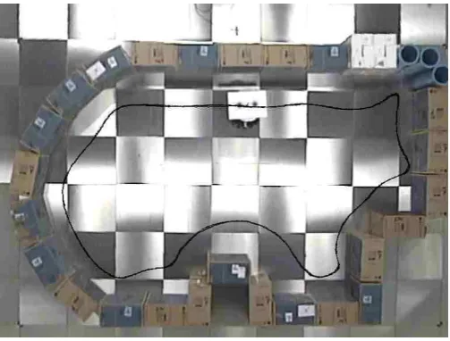
Acquisition of training data First the robot was driven manually using a joystick for half an hour (figure 2). During this time, the coarse coded laser readings and the rotational velocities of the robot were logged every 250ms. The laser perception of the robot was coarse coded in 9 segments by averaging the laser readings over 20◦ _intervals.

Fig. 2.The programmer demonstrates the desired behaviour, wall following, to the robot by driving it manually using a joystick for half an hour. During this time, the coarse coded laser readings and the rotational velocities of the robot were logged every250ms.

Sensor signal encoding The coarse coded laser readings

u1tou9between 0.3 and 0.8 were filtered and normalised

in (0,1) using equation 1 and 2.

nui=max(min(tui,1), 0 ) (1)

where

tui=

(ui−umin)

(umax−umin)

(2)

i = 1· · ·9,nui is normalised laser reading and umax =

0.8,umin= 0.3 are maximum and minimum range of laser

readings respectively. Then the coarse coded and nor-malised laser vector was reduced into two element input vector by extracting the minimum laser reading among all the normalised readings and the reading from the right-most normalised laser reading (equation 3 and 4).

ˆ

u1=min(nui) (3)

ˆ

u2=nu1 (4)

Obtaining sensor-based polynomials After the collection of training data, a polynomial model was obtained, identi-fying the rotational velocityωof the robot as a function of the two filtered laser readings. In order to simplify the ex-periment, the travel speed of the robot was kept constant at 0.15m/s. The model was chosen to be a linear ARMAX polynomial structure of first degree with no regression in the inputs and output (i.e.l = 1, Nu = 0, Ny = 0), and

contained the 3 terms given in table 1.

ω(n) = +0.463−_1.967∗_ˆu1(n) + 0.901∗uˆ2(n)

Table 1

Experiment 1. ARMAX controller which links the coarse-coded laser readings of the robot to its angular velocity to achieve right-hand wall following behaviour (see figure 2).

In table 1 ω(n) is the rotational velocity of the robot (in rad/s) at time instantn, ˆu1(n) is the minimum coarse

coded and normalised laser reading and ˆu2(n) is the right

most coarse coded and normalised laser reading.

Testing the model Having obtained the sensor based con-troller, first, we let the model drive the robot in the train-ing environment for about 15 minutes. The obtained tra-jectory (figure 3) matches the target tratra-jectory (figure 2) very closely.

Fig. 3. Experiment 1: The trajectory of the robot driven by the ARMAX controller given in table 1 resembles the training trajectory (figure 2) very closely.

Then we tested our model for 15 minutes in a different test environment to test the generalisation capability of the model (figure 4). The results are again satisfactory.

4. Robot Training: Method 2

Fig. 4.Experiment 1: Performance of the ARMAX controller in a novel test environment. The results show that the AR-MAX controller captured the fundamental relationship be-tween the coarse coded laser readings and the rotational velocity commands in order to achieve right wall follow-ing behaviour, even in an environment that differed from the training scenario.

([Nehmzow et al., 2007b,Akanyeti et al., 2007b]). This method has 4 stages:

4.1. Programming by Demonstration

(i) Human demonstration: First, the programmer demonstrates the desired behaviour by performing it in the target environment. For the purpose of this paper we confined our experiments to 2-dimensional navigation problems reflecting the motion capabili-ties of our robot (2 degrees of motion, translational and rotational). During this initial demonstration, we log the xand y position of the human user with a sampling rate of 50Hz by using the Vicon motion tracking system. Once the operator’s trajectory is logged, we compute the translational and rotational velocities of the demonstrator by differentiating con-secutive (x, y) samples along the trajectory.

(ii) Sensorless trajectory following In the second stage we use the Narmax system identification method to obtain two sensor-free polynomials, one expressing rotational velocity as a function of time and past rotational velocities, the other expressing the translational velocity as a function of time and past linear velocities.

We then use these two sensor-free polynomials to drive the robot blindly along the trajectory the hu-man had taken earlier, now logging sensor readings and velocities. We use a sampling frequency of 10Hz at this stage.

(iii) Obtaining sensor based controllers The sensor-free controllers obtained at stage II are ballistic con-trollers that drive the robot along the desired trajec-tory, as long as the robot is started from the same ini-tial positions as the human. However, for real-world

applications it is essential that sensor feedback is used to control the motion of the robot.

In the final stage we therefore use the Narmax system identification method to obtain sensor-based controllers, using the previously logged sensor-motor pairings. This controller can subsequently be used to control the robot in the target environment, copy-ing the original behaviour exhibited by the human demonstrator.

(iv) Model validationFinally we let the obtained con-trollers drive the robot in the train and test environ-ments to see if the models capture the necessary re-lationship between the robot’s perception and action in order to achieve the desired behaviour.

4.2. Experiment 2: Corridor Following

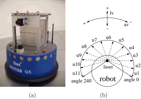
To demonstrate the viability of this second method, we demonstrated to aScitos G5 mobile robot (figure 5) how to follow the U-shaped corridor of 150 cm width shown in figure 6. The human demonstrator started at right side and then walked to the end of the corridor. During this time, the position of human was logged in every 20ms by using theViconmotion tracking system.

robot

angle 240 angle 0 laser

av lv

+

− −

u1 u2 u3 u4 u5 u6 u7 u8

u9

u11 u10

+

(a) (b)

Fig. 5. (a) The Scitos G5 robot Dax. Dax has two degrees of freedom (translational and rotational) and is a Hokuyo laser range finder. The range finder has a wide angular range (240◦_{) with a radial resolution of0.36}◦ _{and distance} resolution of less than 1cm. (b) In order to decrease the dimensionality of the input space to the Narmax model, we coarse coded the laser readings into11sectors (u1 tou11) by averaging 62 readings for each22◦_intervals.

After we estimated the rotational and translational ve-locities of the programmer along the desired trajectory through differentiation of (x,y) positions, we used the Nar-max system identification method to obtain two sensor-free controllers for the translational velocity and the rotational velocity of the robot. Both models are given in table 2.

Fig. 6.Experiment 2: The trajectory of the human demonstra-tor in the U-shaped corridor environment. The width of the corridor is 150 cm.

lv(n) = av(n) = +0.347 −_0.005

+0.004∗_{u(n,1) +0.001}∗_u(n,1) −_0.001∗_u(n,1)2

+0.001∗_u(n,1)2

−_0.001∗_u(n,1)3

+0.818∗_y(n−₁₎

+0.158∗_y(n−₁₎2

−_0.276∗_y(n−₁₎3

+0.001∗_u(n,1)∗_y(n−₁₎ −_0.001∗_u(n,1)2_∗

y(n−₁₎

Table 2

Two sensor-free polynomials to drive the robot “blindly” along the human trajectory given in figure 6. lv(n) is the translational velocity in m/s,av(n)the rotational velocity in rad/s andu(n,1)is time variable at time instantn.

During this run, the laser readings and the robot’s trans-lational and rotational velocities were logged every 100ms.

Sensor Signal Encoding In order to decrease the dimen-sionality of the input space to the Narmax model, we coarse coded the laser readings into 11 sectors by averag-ing 62 readaverag-ings for each 22◦ _{interval. We then used the}

Narmax identification procedure to estimate the robot’s translational and rotational velocities as a function of the coarse coded laser readings (u1,u2,· · ·,u11). Both models

are given in table 3.

Model validation We then validated the sensor-based models given in table 3 by letting them control the robot in the U shaped corridor. We started the robot from 10 different locations, and observed correct corridor following behaviour in all cases. The resulting trajectories are shown in figure 8.

Fig. 7.Experiment 2: The trajectory of the robot under con-trol of the sensor-free polynomials given in table 2. The models drive the robot along the human trajectory given in figure 6 without using any sensory perception. During this run, the robot logs its own perception and velocity com-mands. The logged data is then used to obtain the final, sen-sor-based controllers which link the perception of the robot to motor commands.

lv(n) = av(n) = +1.011 +0.570

−_0.037∗_{u(n,1) +0.002}∗_u(n,1)

+0.164∗_{u(n,2) +0.069}∗_u(n,2)

+0.147∗_{u(n,3) +0.052}∗_u(n,3) −_0.128∗_u(n,4) −_0.181∗_u(n,4) −_0.116∗_u(n,5) −_0.046∗_u(n,5) −_0.051∗_u(n,6) −_0.049∗_u(n,6) −_0.075∗_u(n,7) −_0.038∗_u(n,7) −_0.051∗_u(n,8) −_0.020∗_u(n,9) −_0.074∗_u(n,9) −_0.050∗_u(n,10) −_0.131∗_u(n,10)

Table 3

Two sensor-based polynomials which link the robot’s percep-tion to motor commands in order to achieve the behaviour shown in figure 6.lv(n)and av(n) are the robot’s transla-tional velocity in m/s and rotatransla-tional velocity in rad/s at sampling pointn.u1 tou11 are the laser bins defined in fig-ure 5.

5. Extending Method 2

The experiments presented so far used an external, cam-era based motion tracking system to log trajectory infor-mation. However, such tracking systems are complicated to set up, have to be calibrated, and, most importantly for service robotics applications, are not found in real world environments.

in-Fig. 8. Experiment 2: Ten trajectories of the robot under control of the sensor-based controllers given in table 3. Not the convergence to one stable trajectory, irrespective of starting point.

terpreting camera images through a Narmax model, which was trained to predict the position of the demonstrator from the camera image.

5.1. Demonstrator position estimation, using perceptual features

Our method is based on training a mathematical poly-nomial using the Narmax system identification methodol-ogy which maps the position of a red jacket worn by the demonstrator in the robot’s camera image with the rela-tive position of the demonstrator referenced to the robot coordinate frame (see figure 9 and 10).

Fig. 9. Position estimation models, identifying the relation-ship between the position of the jacket in the image and the position of the demonstrator referenced to the robot’s co-ordinate system.(xmin, ymin)and(xmax, ymax)are the

coor-dinates of the “left up” and “right down” corners of the rectangle surrounding the red jacket (see figure 10 ). These coordinates are computed by separating the red jacket from the background of the image using a blob colouring algo-rithm.

x

y

y

max

x

X axis

Y axis

0,0

(a) (b)

Fig. 10.(a) The output image after a pre-processing stage. The demonstrator’s jacket was isolated from the rest of the image using a blob colouring algorithm. (b) The position information of the jacket is then fed to Narmax models which identify the position of the demonstrator relative to the robot’s reference coordinate.

Finding the position of the jacket Figure 11 shows the block diagram that illustrates how we extract the position of the red jacket from the captured images.

Fig. 11.The block diagram that illustrates how the position of the red jacket is extracted from the captured images. First the lens distortions are removed from the raw image. Then the corrected image is converted into chromaticity space which is less illumination dependent. In the final stage, the jacket is separated from the background of the image by blob colouring algorithm (see figure 10).

First we remove lens distortions from the captured im-ages. Once the image is corrected, we convert it into “chro-maticity colour space” which is less illumination dependent that the RGB colour space (equations 5-7).

Cr= R

R+G+B, (5)

Cg= G

R+G+B, (6)

Cb= B

whereCr,CgandCbare the red chromaticity, green

chro-maticity and blue chrochro-maticity components respectively, andR,GandBare the red, green and blue values respec-tively of the colour to be described.

In the final stage, we separate the jacket from the back-ground of the image by using a blob colouring algorithm. Blob colouring is a technique used to find regions of similar colour in the image. The connected pixels are grouped to-gether if they have similar intensity values and assigned to different regions if the difference in their intensity values is bigger than a certain threshold.

After completion of the blob colouring algorithm we as-sume that the biggest red coloured region corresponds to the red jacket, making sure that assumption holds through our experimental procedure. We then compute the mini-mum rectangular box which can frame the jacket entirely (figure 10). The coordinates of the “left up” and “right down” corners of the rectangle are then fed to Narmax polynomials obtained to predict the position of the demon-strator.

Acquisition of the training data In order to collect train-ing data for the estimation of the programmers’s position during the demonstration, the human trainer wearing a red jacket walked randomly in the robot’s field of view for half an hour. During the training session the robot was station-ary, and the robot’s camera was aligned parallel to the floor so that the robot’s field of view has the maximum coverage area for the demonstrator.

During this time the position of the jacket in the cap-tured images and the relative position of the demonstrator referenced to the robot — obtained through theVicon mo-tion tracking system — were logged synchronously every 250ms. Figure 12 shows the stream of the original and the processed images captured during the training session.

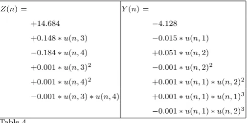
Obtaining position prediction models We then used the Narmax system identification procedure to estimate the rel-ative position of the demonstrator referenced to the robot as a function of the position of the jacket in the image (xmin, xmax, ymin and ymax). TheZ position prediction

model was chosen to be second degree with no regression in the input and output (i.e.l= 2,Nu= 0,Ny= 0). The

re-sulting model contained 6 terms. TheY position prediction model was chosen to be fourth degree with no regression in the input and the output (i.e.l= 4,Nu= 0,Ny = 0) and

contained 7 terms. Both models are given in table 4. Figure 13 shows the predicted and actual position of the demonstrator in the robot’s coordinate frame.

Model validation We compared the predicted position of the demonstrator with the actual position by analysing the error distributions. The results show that the average error between the predicted and actual position of the demon-strator is less than 10mm±3mm for both models (see fig-ure 14).

1 2 3 4

5 6 7 8

Fig. 12.Stream of images captured by the robot’s camera dur-ing the acquisition of the traindur-ing data set used in obtain-ing Narmax model in order to calculate the position of the demonstrator. Each image is pre processed using the proce-dure given in figure 11 in order to extract the position of the red jacket in the image.

Z(n) = Y(n) = +14.684 −_4.128

+0.148∗_u(n,3) −_0.015∗_u(n,1) −_0.184∗_{u(n,4) +0.051}∗_u(n,2)

+0.001∗_u(n,3)2 ₋

0.001∗_u(n,2)2

+0.001∗_u(n,4)2

+0.001∗_u(n,1)∗_u(n,2)2

−_0.001∗_u(n,3)∗_{u(n,4) +0.001}∗_u(n,1)∗_u(n,1)3

−_0.001∗_u(n,1)∗_u(n,2)3

Table 4

Two position polynomials which link the perception of the robot to the position of the demonstrator in the robot’s reference frame.Z(n)andY(n)are thezposition (inm) and

yposition (inm) of the demonstrator at time instantnand

u1 tou4 are thexmin, xmax,ymin and ymax coordinates of

the “red jacket blob” extracted from the image as described in figure 11.

5.2. Experiment 3 Door Traversal

Fig. 13.The predicted and actual position of the demonstra-tor in the robot’s coordinate frame.

Analysis of the observed trajectory reveals that there is noise in the data because of two reasons:

(i) There is a constant oscillation in the motion of the demonstrator, which originates from the swinging motion perpendicular to the heading direction. This is a general characteristic of the two legged locomo-tion in humans.

(ii) The polynomials that compute the position of the demonstrator with respect to the robot are very sen-sitive to how accurate the position and the size of the jacket is extracted from the image. So far we as-sumed that the red jacket is a rectangular, rigid ob-ject; in other words, that the coordinates of the top left and bottom right corners of the jacket would give us the position in the image and the size of the jacket accurately. However the information about the posi-tion and the size can be noisy when the shape of the jacket is deformed due to the shoulder motions of the demonstrator.

We eliminated some noise by using a low pass filter, as-suming that the demonstrator didn’t do sharp changes in the heading direction while performing the desired task. We then computed the translational and rotational velocities

Fig. 14.The error distributions of theZposition prediction model and theY position prediction model. The average er-ror between the predicted and actual position of the demon-strator is less than10mm±_{3mm for both models.}

robot

angle 240 angle 0 laser

av lv

+

− −

u1 u2 u3 u4 u5 u6 u7 u8

u9

u11 u10

+

(a) (b)

REX HUMAN

Fig. 16.Experiment 3: The trajectory taken by the demonstra-tor while passing through the two openings of120cm width. While the demonstrator was performing this behaviour, the robot was observing him and calculating the demonstrator’s relative trajectory according to the robot itself using po-sition prediction models given in table 4.

of the demonstrator along the trajectory.

t=18 t=39 t=50

t=61 t=72 t=80

Fig. 17.Stream of six images captured by the robot’s camera during the demonstration of the desired behaviour. The num-bers below each image indicate the frame number of the im-age (frame rate 4Hz). The captured imim-ages are then pre pro-cessed as described in section 5.1 in order to extract the position of the red jacket.

Having obtained the velocity information of the demon-strator along the desired path, we used them to drive the robot blindly in the test environment. During this first robot interaction with the environment, laser readings and

the robot’s translational and rotational velocities were logged in every 250ms (see figure 18).

REX

Fig. 18.Experiment 3: The trajectory of the robot under the control of the given velocity commands obtained from the human trajectory given in figure 16, not using any sensory perception. During this pass,Rexlogs its own perception per-ceived along the trajectory and the velocity commands. The logged data is then used to obtain sensor-based controllers which link the perception of the robot to the desired be-haviour.

Sensor signal encoding In order to decrease the dimen-sionality of the input space to the Narmax model, we coarse coded the laser readings into 11 sectors by averag-ing 62 readaverag-ings for each 22◦ _{interval. We then used the}

Narmax identification procedure to estimate the robot’s translational and rotational velocities as a function of the coarse coded laser readings (u1,u2,· · ·,u11), see figure 15.

Both the translational and the steering speed model were chosen to be second degree. No regression was used in the inputs and output (i.e.l= 2,Nu= 0,Ny = 0) resulting in

non linear Narmax structures. Both the models contained 18 terms (table 5).

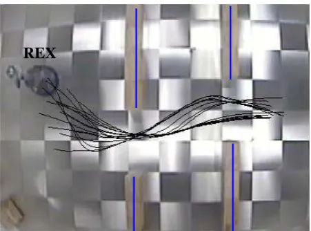
Model validation We then let the sensor based models drive the robot in the test environment starting from 15 dif-ferent locations. Figure 19 shows that the obtained mod-els are successfull in driving the robot through both the door like openings without collisions.

6. Better Position Prediction

lv(n) = av(n) =

−_{0.751 +2.260}

+0.059∗_u(n,3) −_0.054∗_u(n,3)

+0.243∗_u(n,4) −_0.480∗_u(n,4)

+0.040∗_u(n,5) −_0.144∗_u(n,5)

+0.139∗_u(n,6) −_0.637∗_u(n,6)

+0.219∗_u(n,7) −_0.195∗_u(n,7) −_0.040∗_{u(n,8) +0.212}∗_u(n,8) −_0.001∗_u(n,9) −_0.056∗_u(n,9) −_0.003∗_u(n,3)2 ₋

0.003∗_u(n,3)2

−_0.008∗_u(n,4)2

+0.014∗_u(n,4)2

−_0.007∗_u(n,6)2

+0.004∗_u(n,5)2

−_0.024∗_u(n,7)2

+0.085∗_u(n,6)2

+0.008∗_u(n,8)2 ₋

0.029∗_u(n,8)2

−_0.003∗_u(n,9)2

+0.013∗_u(n,9)2

−_0.010∗_u(n,3)∗_{u(n,4) +0.012}∗_u(n,3)∗_u(n,4) −_0.001∗_u(n,3)∗_u(n,5) −_0.004∗_u(n,3)∗_u(n,8) −_0.028∗_u(n,4)∗_{u(n,6) +0.033}∗_u(n,4)∗_u(n,6) −_0.024∗_u(n,4)∗_{u(n,7) +0.050}∗_u(n,4)∗_u(n,7)

Table 5

Experiment 3. Two sensor-based polynomials which link the perception of the robot to the desired behaviour shown in figure 18.lv(n)andav(n)are the translational velocity (in

m/s) and rotational velocity (inrad/s) of the robot at time instantnandu1 tou11are the coarse coded laser readings starting from the right extreme of the robot.

REX

Fig. 19. Experiment 3: The trajectories of the robot under the control of sensor based controllers given in table 5. The robot was started from15different locations and it passed through the both door like openings successfully.

the camera, it is almost impossible to do so consis-tently, and some noise is thereby introduced. (ii) The jacket takes the form of the programmer’s body,

therefore the size and the shape of the jacket does not only depend on the position of the programmer, but also on body form and demonstrator movements. We therefore decided to track an orange sphere, rather than the red jacket, because the perception of a sphere is

orientation-independent.

6.1. Position prediction using an orange ball

For narrow angle view and good quality cameras like the one mounted on the robot, we can assume that the perspective projections of the ball correspond to circular regions on the image plane regardless of the position and the orientation of the ball in the real world. Therefore:

(i) The radius of the circular region on the image plane is directly proportional with the radius of the ball and inversely proportional to the distance between the ball and the robot’s camera. As the ball is fur-ther away from the camera, the size and fur-therefore the radius of the ball get smaller and vice versa.

(ii) The perspective projection of the ball is independent from the orientation of the ball, therefore during the demonstration the programmer does not have to face the camera all the time.

Based on the above assumptions, the relative position of the ball according to the robot can be computed as:

ballz= R

r ∗f (8)

bally= R

r ∗yc (9)

whereballzandballyare the relativezandypositions of

the ball centre according to the robot,Ris the diameter of the ball in the real world,ris the diameter of the circular region on the image plane corresponding to ball,yc is the y pixel coordinate of the ball silhouette on the image and

f is the focal length of the camera (figure 20).

Fig. 20.The perspective projection of the ball on the image plane whereRandrare the diameter of the ball and ball silhouette on the image plane respectively.

Training position prediction models We did not use intrin-sic camera parameters such as focal length and the image centre of the camera, but decided to train an ARMAX poly-nomial in the same form with theoretical formulae given in equations 8 and 9 to identify the coefficients of the formu-lae without needing to know the camera parameters.

orange ball walked randomly in the robot’s field of view for half an hour. During the training session the robot was stationary, and the robot’s camera was aligned parallel to the floor so that the robot’s field of view had maximum coverage area for the demonstrator.

During this time the position and the radius of the ball in the captured images and the relative position of the demon-strator referenced to the robot — obtained through the Vi-con motion tracking system — were logged synchronously every 100ms. Figure 21 shows stream of original and the processed images captured during the training session.

1 2 3 4

5 6 7 8

Fig. 21. Stream of images captured by the robot’s camera during the training session. The captured images are then preprocessed to compute the position and the diameter of the ball in the image (see also figure 22).

In order to find the centre and the radius of the ball in the images, we modified the blob colouring algorithm — previously described in section 5.1 — in such a way that it extracted the biggest orange coloured region in the image (figure 22).

We then used an ARMAX system identification process to find the coefficients of the theoretical formulae which express the relative position of the ball with respect to the robot coordinate frame in the real world as a function of the position and the diameter of the ball silhouette in the image. The resulting models are given in table 6, withZ(n) being the position of the ball in z direction, Y(n) is the position of the ball inydirection (figure 20),uz(n) is

1

r and uy(n) being y

c

r at time instantn.

Figure 23 shows the actual and predicted positions of the ball in the robot’s coordinate frame.

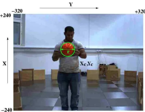
Models analysis and validation The analysis of theZ po-sition prediction graph in figure 23 confirms the expecta-tion that predicexpecta-tion gets worse as the distance between ball and camera increases. As the apparent diameter of the ball decreases prediction models become more sensitive.

Fig. 22. Once the image is captured, the ball is extracted from the image using a blob colouring algorithm whereXc

andYc are the centre position andris the diameter of the

ball in the blob image.

Z(n) = Y(n) = +128.321 −_63.429

+145792.540∗_uz(n) −_209.167∗_uy(n)

Table 6

Two position predictors which model the ball’szandy po-sitions (in mm) within the robot’s coordinate system as a function of the ball’s image positions.uz(n)is 1_r anduy(n)is yc

r at time instantn.

In order to find out how sensitive the performance of theZposition predictor is to the smallest possible error of “one pixel” we took the first derivative of theZ position prediction model with respect to the diameter of the ball:

dZ duz

= −145792.540

u2

z

(10)

and plotted the resultant equation (equation 10) for dif-ferent diameter values varying between 20 pixels (when the ball is approximately 6 metres away from the camera) to 140 pixels (when the ball is approximately 1 meter away from the camera) .

The resulting graph (figure 25) confirms our expectation that the performance of the prediction model is very robust when the ball is close to the camera. When the distance between the camera and the ball is around 1m, the diameter of the ball in the camera image is around 140 pixels and the error between the actual and the predicted position for one pixel miscalculation error is less than a centimetre. As the ball gets further away from the camera, the performance of the position prediction model drops drastically. When the diameter of the ball is around 20 pixels (the ball is approximately 6m away from the camera) the one pixel miscalculation of the ball’s diameter causes approximately 35cm error in predicting the position.

Comparing performance using the two different markers

ac-Fig. 23.The predicted (red) and actual position (blue) of the ball in the robot’s coordinate frame given in figure 20

tual and the predicted positions of the demonstrator in the

y and z directions (figure 26). When we compare the er-ror distributions of the two position prediction models ob-tained for the orange ball with the two models obob-tained for the red jacket we see that the red jacket’s models with an average 10mm±3mm are significantly more accurate in predicting the position of the programmer than the models obtained for the orange ball with an average 100mm±3mm (U-test, p<0.05).

This is because the red jacket is bigger than the orange ball, therefore the models obtained for the orange ball are more sensitive to the noise introduced by the blob colouring algorithm.

Fig. 24.These figures show how the diameter of the ball sil-houette on the image plane is related to the relative posi-tion of the ball according to the camera. As the ball goes further away from the camera, the diameter of the ball on the image plane gets smaller and vice versa.

6.2. Experiment 4: Route Learning

After obtaining position prediction models, we tested the viability of the models by teachingRex(figure 15) to follow a user-specified route in the environment given in figure 27. The programmer walked once to show the robot the desired route. During this time, the robot calculated the position of the demonstrator, using the position prediction models given in table 6 every 100ms. Figure 28 shows a stream of images which were captured and used by the robot to obtain the position information of the programmer during the demonstration.

Fig. 25.The plot of dZ duz =

−145792.540

u2z

whereuz, the diameter

of the ball in the image, varies between 20 and 140. This graph indicates how much error would be expected from the performance of the Zposition prediction model for a “one pixel error” with respect to the true diameter of the ball.

robot’s translational and rotational velocities were logged in every 100ms (figure 29).

Obtaining sensor based polynomials As in the previous door traversal experiment described in section 5.2, we coarse coded the laser readings into 11 sectors by averaging 62 readings for each 22 degree intervals in order to de-crease the dimensionality of the input space to the Narmax model. We then used the Narmax identification procedure to estimate the robot’s translational and rotational veloc-ities as a function of the coarse coded laser readings (u1,

u2,· · ·,u11(see figure 15)).

Both the translational and the steering speed model were chosen to be second degree. No regression was used in the inputs and output (i.e. l = 2, Nu = 0, Ny = 0)

result-ing in non linear Narmax structures. The linear velocity model contained 43 terms and the angular velocity model contained 40 terms (table 7).

Model analysis and validation Having obtained the mod-els given in table 7, we used them to drive the robot in the test environment starting from 10 different locations. Figure 30 shows that the obtained models successfully ne-gotiate the route, but that in three runs the robot did not finish at the exact route endF.

We observed that the obtained perception models are not robust, but sensitive to small perturbations, such as the initial starting positions of the robot. Along the desired trajectory the relationship between the robot’s perception and the desired motor responses vary, depending on the robot’s position along the trajectory. For example when the robot is in regionA(figure 31) the sensors on the right side of the robot are more important than the rest in obtaining

Fig. 26. The error distributions of the position prediction models obtained for predicting the position of the orange ball. Compared with the performance of the models obtained for the red jacket (figure 14), we see that the red jackets models with an average 10mm±_{3mm are significantly more}

accurate in predicting the position of the programmer than the models obtained for the orange ball with an average

100mm±_{3mm (U-test, p<0.05).}

1 2 3 4

5 6 7 8

Fig. 28. Stream of images captured by the robot’s camera during the demonstration of the desired route following behaviour.

Fig. 29.Experiment 4: The trajectory of the robot while fol-lowing the desired route blindly (figure 27). During this run, the robot logs its own perception and the desired velocity commands every 100ms. The logged data were then used in the training of NARMAX polynomials to obtain sensor-based controllers given in table 7.

Fig. 30. Experiment 4: The trajectories of the robot under the control of the sensor-based polynomials given in table 7. During the experiments the robot was started from 10 dif-ferent locations. The robot completed the route in all ten cases, but in three cases did not finish at locationF.

lv(n) = +0.218 av(n) = −_0.608 −_0.008∗_{u(n,1) +0.059}∗_u(n,1) −_0.109∗_u(n,2) −_0.178∗_u(n,2)

+0.071∗_u(n,3) −_0.070∗_u(n,3) −_0.075∗_{u(n,5) +0.040}∗_u(n,4) −_0.039∗_{u(n,6) +0.032}∗_u(n,5)

+0.132∗_{u(n,7) +0.089}∗_u(n,6)

+0.029∗_{u(n,8) +0.264}∗_u(n,7) −_0.037∗_{u(n,9) +0.235}∗_u(n,8) −_0.045∗_u(n,10) −_0.110∗_u(n,9) −_0.092∗_u(n,11) −_0.080∗_u(n,10)

+0.010∗_u(n,1)2 ₋

0.100∗_u(n,11)

+0.023∗_u(n,2)2

+0.008∗_u(n,1)2

−_0.015∗_u(n,3)2

+0.037∗_u(n,2)2

+0.001∗_u(n,4)2

+0.030∗_u(n,3)2

+0.007∗_u(n,5)2 ₋

0.002∗_u(n,4)2

+0.003∗_u(n,6)2 ₋

0.009∗_u(n,5)2

−_0.029∗_u(n,7)2 ₋

0.017∗_u(n,6)2

−_0.005∗_u(n,8)2 ₋

0.047∗_u(n,7)2

+0.010∗_u(n,9)2 ₋

0.025∗_u(n,8)2

+0.014∗_u(n,10)2

+0.030∗_u(n,9)2

+0.016∗_u(n,11)2

+0.025∗_u(n,10)2

−_0.006∗_u(n,1)∗_{u(n,2) +0.020}∗_u(n,11)2

+0.001∗_u(n,1)∗_{u(n,4) +0.001}∗_u(n,1)∗_u(n,2) −_0.004∗_u(n,1)∗_u(n,6) −_0.020∗_u(n,1)∗_u(n,3) −_0.001∗_u(n,1)∗_u(n,7) −_0.022∗_u(n,1)∗_u(n,5) −_0.003∗_u(n,1)∗_u(n,8) −_0.004∗_u(n,1)∗_u(n,6) −_0.001∗_u(n,2)∗_{u(n,4) +0.004}∗_u(n,1)∗_u(n,7)

+0.001∗_u(n,2)∗_{u(n,5) +0.004}∗_u(n,1)∗_u(n,9)

+0.005∗_u(n,2)∗_{u(n,6) +0.001}∗_u(n,1)∗_u(n,10)

+0.008∗_u(n,2)∗_{u(n,7) +0.008}∗_u(n,2)∗_u(n,3) −_0.001∗_u(n,2)∗_{u(n,8) +0.001}∗_u(n,2)∗_u(n,5) −_0.003∗_u(n,2)∗_u(n,9) −_0.008∗_u(n,3)∗_u(n,8) −_0.005∗_u(n,2)∗_u(n,10) −_0.001∗_u(n,4)∗_u(n,5)

+0.002∗_u(n,3)∗_u(n,4) −_0.003∗_u(n,4)∗_u(n,7) −_0.003∗_u(n,3)∗_u(n,8) −_0.004∗_u(n,4)∗_u(n,9) −_0.002∗_u(n,4)∗_{u(n,10) +0.027}∗_u(n,5)∗_u(n,6)

+0.005∗_u(n,5)∗_u(n,6) −_0.008∗_u(n,5)∗_u(n,9)

+0.009∗_u(n,5)∗_u(n,8) −_0.011∗_u(n,7)∗_u(n,10) −_0.003∗_u(n,5)∗_u(n,9) −_0.031∗_u(n,8)∗_u(n,10)

+0.002∗_u(n,5)∗_u(n,11)

+0.004∗_u(n,6)∗_u(n,8)

+0.005∗_u(n,6)∗_u(n,11)

Table 7

the desired motor response (figure 32). In region B, the sensors in front of the robot become more important and in regionCthe sensors on the left side of the robot are more important.

Fig. 31.Experiment 4: The relationship between the robot’s perception and the desired actions is dependent on the posi-tion of the robot along the route.

Fig. 32. Experiment 4: This figure shows how the contribu-tions of the sensors around the robot to obtain the desired motor response changes along the desired route. In region

Athe sensors on the right side of the robot are more impor-tant than the rest. As the robot enters regionBthe sensors in front of the robot are more correlated with the desired motor response. Finally, in regionCthe sensors on the left side of the robot become more dominant for the desired mo-tor response.

We are currently investigating how to address this prob-lem. On straightforward method would be to represent complex, time-dependent sensor-motor tasks by a several polynomial models, using a classifier which divides the perception-action space of the robot into subspaces and generates a separate model for each subspace. This method has already been seen to work in initial experiments at Es-sex. We are, however, also investigating ways of represent-ing complex tasks inonemodel; this is work in progress.

7. Conclusion and Future Work

This paper discusses robot experiments aiming at devel-oping a formal, theory based design methodology to gen-erate transparent robot control programs using mathemat-ical functions. The research finds its theoretmathemat-ical roots in robot training and system identification techniques such as Armax (Auto-Regressive Moving Average models with eX-ogenous inputs) and Narmax (Non-linear Armax).

In the first set of experiments ([Nehmzow et al., 2005], [Kyriacou et al., 2006] and [Akanyeti et al., 2007a]), we

operate the robot manually, using a joystick, to follow a desired trajectory. Once training data is acquired in this way, we use the NARMAX modelling approach to obtain a model which identifies a coupling between sensory per-ception and motor response as a polynomial model. This model is then used to control the robot autonomously.

In ([Nehmzow et al., 2007b] and [Akanyeti et al., 2007b]) we introduced a new mechanism to program robots — pro-gramming by demonstration — based on algorithmically translating observed human behaviours into robot control code, using transparent system identification techniques. To obtain such sensor-motor controllers, we first demon-strate the desired motion to the robot by walking in the target environment. Using this demonstration, we obtain recurrent, sensor free models that allow the robot to fol-low the same trajectory blindly. During this motion the robot logs its own perception-action pairs, which are sub-sequently used as training data for the Narmax modelling approach that determines the final, sensor-based models which identify the coupling between sensory perception and motor responses as non linear polynomials. These models are then used to control the robot.

Previously we used an external, camera-based motion tracking system to log the trajectory of the human demon-strator during his initial demonstration of the desired mo-tion. However, besides being expensive, such tracking sys-tems are complicated to set up and not always available.

We therefore improved our training method by replac-ing theVicon motion tracking system with Narmax poly-nomial models which are trained to predict the position of the red jacket worn by the demonstrator using the robot’s own vision system [Nehmzow et al., 2007a]. The statistical analysis showed that the obtained models are able to pre-dict the position of the demonstrator in our laboratory with an accuracy of 10mm±3mm.

We compared the position prediction models obtained for two different markers, a red jacket and an orange ball. Even though the jacket is a non-rigid object, its larger size results in more accurate predictions can be made with the relatively small ball: the larger object size makes the posi-tion estimaposi-tion models less sensitive to the noise introduced by the blob colouring algorithm.

Our experiments in modelling time-variant sensor motor tasks using a NARMAX system identification technique also show that using single models to represent complex sensor-motor tasks (such as entire long routes) may not be viable, and dividing perception-action spaces into sub-spaces may be needed.

7.1. Future work

Ongoing work in our laboratories addresses the following three issues:

Automatic parameter selection for NARMAX methodology

theo-retical knowledge of robot programming, the need for model structure identification remains.We are interested to auto-mate this process.

Object Tracking under occlusion So far our position esti-mation models only take the current image into account. This can be brittle in cases where the tracked object is ei-ther under occlusion or not visible in the image. We ei- there-fore are currently investigate methods of integrating extra information about the tracked object into the model (such as the previous position of the ball and the velocity of the ball), and expect improved performance in cases of occlu-sion.

Generating multi-polynomial sensor-motor couplings As discussed in the previous section, if the sensor-motor task under investigation is time-dependent or very complex, it may not be possible to represent the whole sensor-motor re-lationship in a single model. We therefore currently investi-gate ways of automatically clustering the perception-action space into subspaces, and generating a separate model for each of the subspaces.

The work already carried out and that proposed forms part of our ongoing research to develop a theory of robot-environment interaction.

Acknowledgements

We thank to Theocharis Kyriacou, Roberto Iglesias and Christoph Weinrich for their contributions to this work. We gratefully acknowledge that the RobotMODIC project was supported by the Engineering and Physical Sciences Research Council under grant GR/S30955/01.

References

[Akanyeti et al., 2007a] Akanyeti, O., Kyriacou, T., Nehmzow, U., Iglesias, R., and Billings, S. (2007a). Visual task identification and characterisation using polynomial models. Robotics and Autonomous Systems.

[Akanyeti et al., 2007b] Akanyeti, O., Nehmzow, U., Weinrich, C., Kyriacou, T., and Billings, S. (2007b). Programming mobile robots by demonstration through system identification. InECMR, Freiburg, Germany.

[Allissandrakis et al., 2005] Allissandrakis, A., Nehaniv, C., Dautenhahn, K., and Saunders, J. (2005). An approach for programming robots by demonstration: Generalization across different initial configurations of manipulated objects. In

In Proceedings of the IEEE international symposium on computational intelligence in robotics and automation, pages 61– 66.

[Billings and Chen, 1998] Billings, S. and Chen, S. (1998). The determination of multivariable nonlinear models for dynamical systems. In Leonides, C., (Ed.), Neural Network Systems, Techniques and Applications, pages 231–278. Academic press. [Billings and Voon, 1986] Billings, S. and Voon, W. S. F. (1986).

Correlation based model validity tests for non-linear models.

International Journal of Control, 44:235–244.

[Calinon and Billard, 2007] Calinon, S. and Billard, A. (2007). What is the teacher’s role in robot programming by demonstration? toward benchmarks for improved learning. Interaction studies, special issue on psychological benchmarksin human-robot interaction., 8:3 In press.

[Demiris and Hayes, 1996] Demiris, J. and Hayes, G. (1996). Imitative learning mechanisms in robots and humans. InProc. 5th European Workshop on Learning Robots, pages 9–16, Bari, Italy. [Demiris and Johnson, 2003] Demiris, Y. and Johnson, M. (2003).

Distributed, predictive perception of actions: biologically inspired robotics architecture for imitation. CONNECTION SCIENCE, 15(4):231–243.

[Hayes and Demiris, 1994] Hayes, G. and Demiris, J. (1994). A robot controller using learning by imitation. InProc. 2nd Int. Symposium on Intelligent Robotics Systems, pages 198–204, Grenoble, France. [Iglesias et al., 2005] Iglesias, R., Kyriacou, T., Nehmzow, U., and Billings, S. (2005). Robot programming through a combination of manual training and system identification. InProc. of ECMR 05 - European Conference on Mobile Robots 2005.Springer Verlag. [Korenberg et al., 1988] Korenberg, M., Billings, S., Liu, Y. P., and

McIlroy, P. J. (1988). Orthogonal parameter estimation algorithm for non-linear stochastic systems.International Journal of Control, 48:193–210.

[Kyriacou et al., 2006] Kyriacou, T., Akanyeti, O., Nehmzow, U., Iglesias, R., and Billings, S. (2006). Visual task identification using polynomial models. InTAROS, Guildford, UK.

[Nehmzow, 1995] Nehmzow, U. (1995). Applications of robot training: Clearing, cleaning, surveillance. Salford, UK.

[Nehmzow, 2003] Nehmzow, U. (2003).Mobile Robotics: A practical introduction. Springer Verlag, 2nd edition.

[Nehmzow et al., 2007a] Nehmzow, U., Akanyeti, O., Weinrich, C., Kyriacou, T., and Billings, S. (2007a). Learning by observation through system identification. InTAROS, Aberystwyth, Wales. [Nehmzow et al., 2007b] Nehmzow, U., Akanyeti, O., Weinrich, C.,

Kyriacou, T., and Billings, S. (2007b). Robot programming by demonstration through system identification. InIROS, San Diego, USA.

[Nehmzow et al., 2005] Nehmzow, U., Kyriacou, T., Iglesias, R., and Billings, S. (2005). Self-localisation through system identification. InProc. of ECMR 05 - European Conference on Mobile Robots 2005.Springer Verlag.

[Nguyen and Widrow, 1990] Nguyen, D. and Widrow, B. (1990). The truck backer-upper: An example of self-learning in neural networks. pages 287–299.

[Pardowitz et al., 2007] Pardowitz, M., Knoop, S., Dillmann, R., and Zoellner, R. (2007). Incremental learning of tasks from user demonstrations, past experiences and vocal comments. IEEE TRANSACTIONS ON SYSTEMS MAN AND CYBERNETICS PART B, 2:322–332.

[Pomerleau, 1993] Pomerleau, D. (1993).Neural Network Vision for Robot Driving.

[Schaal, 1997] Schaal, S. (1997). Learning from demonstration. In