Improving the localisation accuracy of AUVs operating in highly variable environmental conditions

(1)

Improving the localisation accuracy of AUVs

operating in highly variable environmental

conditions

by

Supun Anuradhitha Tilakeratne Randeni Pathiranachchilage BEng (Hons) in Naval Architecture, University of Tasmania, 2013

A thesis submitted in fulfilment of the requirement for the degree of Doctor of Philosophy

in

Maritime Engineering

National Centre for Maritime Engineering and Hydrodynamics, Australian Maritime College (AMC), University of Tasmania.

(2)

Abstract

The objective of this thesis is to contribute to Autonomous Underwater Vehicle (AUV) navigation by improving vehicle localisation accuracy when Doppler Velocity Log (DVL) bottom-tracking is unavailable. The Inertial Navigation System (INS) based localisation solution is prone to extreme uncertainties due to double integration of inherent errors within the INS acceleration measurements, unless the solution being externally aided (e.g. velocity measurements using the DVL bottom-track). As a solution for this, an improved model-aided INS localisation technique is introduced, which is complimented with the development of a novel model calibration and new water column velocity estimation method. The techniques established in this project are tested and validated using experimental data from a set of field manoeuvres using a Gavia class AUV and the performance is compared against other

commonly used localisation methods.

A baseline mathematical model was developed in this work using system identification to predict the motion response of the AUV based on its control commands. However, such models are generally calibrated for low water column velocities and a standard vehicle configuration, and are limited in application for variations in environmental conditions. To address this limitation, a novel model calibration technique was established to field calibrate the parameters within the baseline model to the current operating condition and vehicle configuration. Model calibration improved the results of the baseline model up to 73% when operating in low energy environments and the AUV position can be computed within an uncertainty range of 1.5% of the distance travelled. In comparison, uncertainties of conventional non-bottom-tracking localisation techniques could be up to 10% in similar environmental conditions. A secondary approach is also presented to determine the hydrodynamic coefficients of the mathematical model using Computational Fluid Dynamics (CFD) simulations and captive model experiments when the AUV is operating in complex flow conditions.

(3)

with water column velocity prediction method, the localisation error is limited to less than 6% of the distance travelled even in extremely high currents (i.e. >2 m s-1 in tested conditions). In such environmental conditions, the uncertainties of other commonly used non-bottom-tracking localisation methods, as tested against in this work, such as DVL water-track mode and unaided INS could be above 30%.

(4)

Declarations

Declaration of originality and authority of access

This thesis contains no material which has been accepted for a degree or diploma by the university or any other institution, except by way of background information and duly acknowledged in the thesis, and to the best of my knowledge and belief no material previously published or written by another person except where due acknowledgement is made in the text of the thesis, nor does the thesis contain any material that infringes copyright.

This thesis may be made available for loan and limited copying and communication in accordance with the Copyright Act 1968.

(5)

Statement of published work contained in thesis

The publishers of the research articles comprising the Chapter 2 to Chapter 4 and Appendix A to Appendix C hold the copyright for that content, and access to the material should be sought from the respective journals and conference proceedings. Chapter 5 is submitted and under review at the time of writing, and may be made available for loan and limited copying and communication in accordance with the Copyright Act 1968.

Statement of co-authorship

The following researchers contributed to the publication of work undertaken as part of this thesis:

 Supun A. T. Randeni P., (Candidate) – Australian Maritime College, University of Tasmania, Launceston, Australia.

 Assistant Prof. Alexander L. Forrest, (AF) – Department of Civil and Environmental Engineering, University of California – Davis, Davis, California, USA and Australian Maritime College, University of Tasmania, Launceston, Australia.

 Dr. Zhi Q. Leong, (ZL) – Australian Maritime College, University of Tasmania, Launceston, Australia.

 Dr. Remo Cossu, (RC) – School of Civil Engineering, University of Queensland, Brisbane, Australia and Australian Maritime College, University of Tasmania, Launceston, Australia.

 Prof. Dev Ranmuthugala (DR) – Australian Maritime College, University of Tasmania, Launceston, Australia.

 Mr. Peter D. King, (PD) – Australian Maritime College, University of Tasmania, Launceston, Australia.

 Mr. Val Schmidt, (VS) – Centre for Coastal and Ocean Mapping, University of New Hampshire, Durham, New Hampshire, USA.

 Dr. Jonathan Duffy (JD) – Australian Maritime College, University of Tasmania, Launceston, Australia.

(6)

 Dr. Hung D. Nguyen (HN) – Australian Maritime College, University of Tasmania, Launceston, Australia.

 Associate Prof. Jonathan Binns (JB) – Australian Maritime College, University of Tasmania, Launceston, Australia.

 Associate Prof. Shuhong Chai (SC) – Australian Maritime College, University of Tasmania, Launceston, Australia.

Chapter 2 – (Paper 1 – published in the Nonlinear Dynamics journal)

Parameter identification of a nonlinear model: replicating the motion response of an autonomous underwater vehicle for dynamic environments

Candidate was the primary author who conducted the design and analysis of the work while all co-authors assisted with refinements and presentation. Candidate, Assistant Prof. Forrest and Dr. Cossu were involved in the AUV deployment and data acquisition.

[Candidate: 75%, AF: 5%, RC: 5%, ZL: 5%, DR: 5%, VS: 5%]

Chapter 3 (Paper 2 – published in the Journal of Marine Science and Engineering)

Determining the Horizontal and Vertical Water Velocity Components of a Turbulent Water Column Using the Motion Response of an Autonomous Underwater Vehicle

Candidate was the primary author and he conducted the design of the technique and analysis together with Assistant Prof. Forrest and Dr Cossu. Co-authors assisted with refinements and presentation. Candidate, Assistant Prof. Forrest and Dr. Cossu were involved in the AUV deployment and data acquisition.

[Candidate: 70%, AF: 10%, RC: 10%, ZL: 5%, DR: 5%]

Chapter 4 (Paper 3 – published in the Marine Technology Society Journal)

(7)

Candidate was the primary author and he conducted the design and analysis. Co-authors assisted with refinements and presentation. Candidate, Assistant Prof. Forrest and Dr. Cossu were involved in the AUV deployment and data acquisition.

[Candidate: 80%, AF: 5%, RC: 5%, ZL: 5%, PD: 2.5% DR: 2.5%]

Chapter 5 (Paper 4 – submitted for publication in the IEEE Journal of Oceanic

Engineering)

Counteracting Autonomous Underwater Vehicle (AUV) localisation error as a precursor for blue water navigation

Candidate was the primary author and he conducted the design of the technique and analysis. Co-authors assisted with refinements and presentation. Candidate, Assistant Prof. Forrest and Dr. Cossu were involved in the AUV deployment and data acquisition.

[Candidate: 80%, AF: 5%, ZL: 5%, RC: 2.5%, DR: 2.5%, PD: 2.5%, VS: 2.5%]

Appendix A (Paper 5 – published in the proceedings of the ‘MTS/IEEE Oceans 2015’)

Estimating flow velocities of the water column using the motion response of an Autonomous Underwater Vehicle (AUV)

Candidate was the primary author and he conducted the design of the technique and analysis together with Assistant Prof. Forrest and Dr. Cossu. Co-authors assisted with refinements and presentation. Candidate, Assistant Prof. Forrest and Dr. Cossu were involved in the AUV deployment and data acquisition.

(8)

Appendix B (Paper 6 – published in the proceedings of the ‘Third Vietnam Conference

on Control and Automation’)

Least Squares Optimisation Algorithm Based System Identification of an Autonomous Underwater Vehicle

Candidate was the second author of this publication. He assisted Mr Minh Tran to conduct the design and analysis of the work and was involved in the AUV deployments.

[MT: 75%, Candidate: 10%, HN: 5% JB: 5%, SC: 2.5%, AF: 2.5%]

Appendix C (Paper 7 – published in the Applied Ocean Research journal)

Numerical Investigation of the Hydrodynamic Interaction between Two Underwater Bodies in Relative Motion

Candidate was the primary author who conducted the experiments, numerical simulations and analysis of the work. Dr. Leong assisted with numerical simulations and all co-authors assisted with refinements and presentation.

(9)

We the undersigned agree with the above stated “proportion of work undertaken” for each of the above published (or submitted) peer-reviewed manuscripts contributing to this thesis

Signed:

……... Dr. Zhi Q. Leong (Primary Supervisor) Australian Maritime College,

University of Tasmania 28/11/2017

……... Assistant Prof. Alexander L. Forrest

(Co-supervisor)

Department of Civil and Environmental Engineering,

University of California – Davis. 28/11/2017

……... Dr. Remo Cossu

(Co-supervisor) School of Civil Engineering,

University of Queensland. 28/11/2017

……... Prof. Dev Ranmuthugala

(Co-supervisor) Australian Maritime College,

University of Tasmania 28/11/2017

……... Associate Prof. Michael Woodward

(Director)

National Centre for Maritime Engineering and Hydrodynamics, Australian Maritime

(10)

Acknowledgements

Over the wonderful journey of my PhD, I have encountered many inspiring and helpful people from around the world and it is a great pleasure to thank them who made this thesis possible.

First and foremost I would like to thank my supervisors Assistant Prof. Alex Forrest, Dr. Zhi Leong, Dr. Remo Cossu and Prof. Dev Ranmuthugala for their unconditional support in all my endeavours. Throughout my PhD journey, they provided me encouragement, sound advices and also good company. Without them, this challenging journey would not be a success. Secondly I would like to thank Peter king, Nathan Kemp (currently at Blue Ocean Monitoring Pty. Ltd.), Isak Bowden-Floyd, Dr. Konrad Zurcher and Dr. Damien Guihen from the Autonomous Maritime Systems Laboratory at AMC, not only for their immense support for AUV deployments, but also for the moments we shared; talking about engineering, science and robotics. A special recognition must be made to Dr. Hordur Johannsson and Helgi Thorgilsson at Teledyne Gavia for their continued technical support and assistance throughout this project. I specially thank Val Schmidt from the Centre for Coastal & Ocean Mapping at University of New Hampshire for his directions. Similarly I thank Associate Prof. Karl Sammut, Dr. Andrew Lammas and their team at Flinders University for facilitating me to broaden my experience to autonomous surface vessels and for the adventures we shared in Singapore during Maritime RobotX Challenge 2014. I am grateful to Associate Prof. Art Trembanis for providing me the opportunity to validate my techniques using different vehicle platforms. I also thank his team including Carter DuVal, Kenny Haulsee and Stephanie Dohner at University of Delaware for their support during the AUV deployments and for the welcome I received in Delaware. I also acknowledge Korea Polar Research Institute with special thanks to Dr. Won Sang Lee, Dr. Sukyoung Yun and their team; and Fiona Elliott (National Institute of Water and Atmospheric Research), Lauren Roche (National Oceanic and Atmospheric Administration), Carson Witte and Una Miller (Columbia University) for our adventures in Antarctica. I warmly thank my colleagues at AMC who were not only co-workers, but also great friends who created a very memorable time at AMC.

(11)

(12)

List of Figures

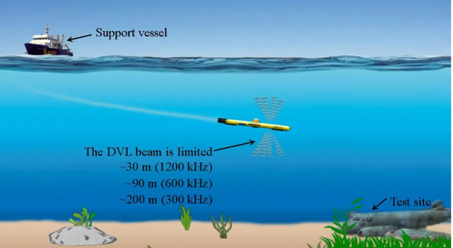
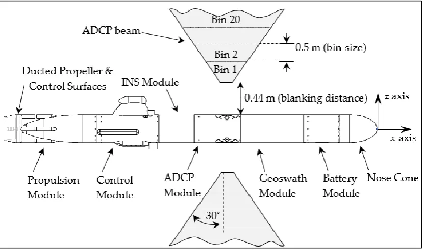
Figure 1.1 – An AUV descends to a test site in blue water where the altitude is larger than the maximum range of the DVL. ... 26 Figure 2.1 – Body-fixed frame of reference and the configuration of the utilised Gavia AUV.

The origin is located at the centre of buoyancy of the vehicle. The vehicle had a length of 2.7 m, a diameter of 0.2 m, and a dry weight in air of approximately 70 kg ... 39 Figure 2.2 – AUV field deployments were conducted (a) in Lake Trevallyn, Tasmania,

Australia and (b) Lake Ohau, South Island, New Zealand. Parameters of the mathematical model were determined from the manoeuvres conducted in Lake Trevallyn. The estimated models were verified with the vehicle motion response data from AUV deployments in Lake Ohau - eight AUV runs were conducted in a lawn-mover pattern (inset). (c) Bathymetry along the AUV Run 1, conducted in Lake Ohau, New Zealand ... 41 Figure 2.3 – Three types of manoeuvres were conducted in Lake Trevallyn site; i.e., zig-zag

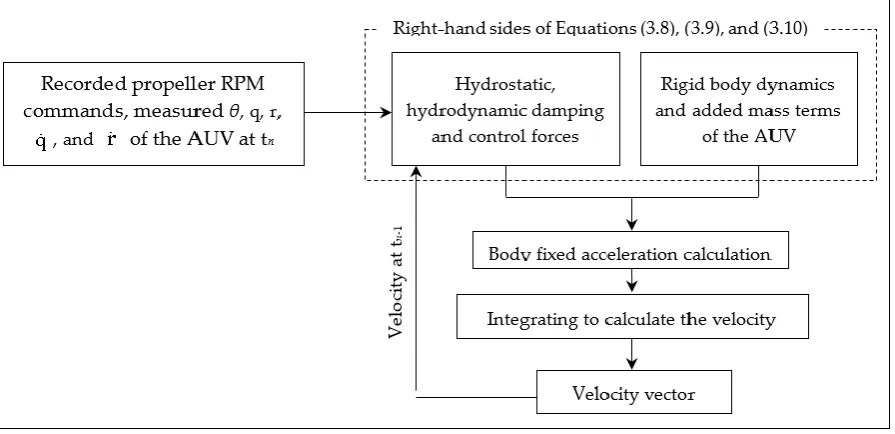
manoeuvres in yaw plane (section shaded in dark grey) and pitch plane (shaded in light grey), and step changes of propeller speed from 450RPM to 975RPM (no shading) . 43 Figure 2.4 – Simulation model flowchart. The solution for the acceleration vector of the current

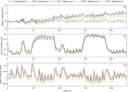
time-step is determined using the control command vectors and velocity vectors from the previous time-step. The velocity vector is then calculated by integrating the acceleration vector with respect to time. *The parameter vector remains constant for non-real time identification ... 51 Figure 2.5 – Comparison between the baseline models and experimental velocities of the AUV

in (a) x, (b) y and (c) z directions for the Lake Trevallyn field tests ... 56 Figure 2.6 – Comparison of the baseline and calibrated model-aided INS velocities in (a) x, (b)

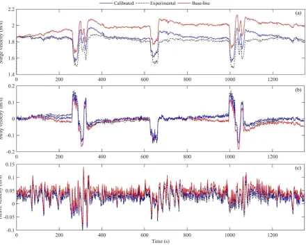
y and (c) z directions against those from the DVL aided INS for the Lake Ohau runs 2 and 3 ... 58 Figure 2.7 – (a) two dimensional AUV paths of Lake Trevallyn manoeuvres derived from the

(19)

typical DVL bottom-track aided INS) while grey and light grey regions show that of 1.5% and 4.0% (i.e., the localisation error level of an DVL water-track-aided INS) .. 61 Figure 3.1 – Configuration of the utilised Gavia AUV with the ADCP beam geometry as

indicated. ... 70 Figure 3.2 – (a) The two experimental field sites in Tasmania, Australia (inset). (b) The Batman

Bridge site with the direction of dominant tidal current flow as shown with solid straight-line arrows. AUV tracks are illustrated with dotted arrows. (c) The Lake Trevallyn site with low turbulence conditions. AUV missions were conducted along the dotted line... 72 Figure 3.3 – The WVAM method flowchart to predict water column velocities from the

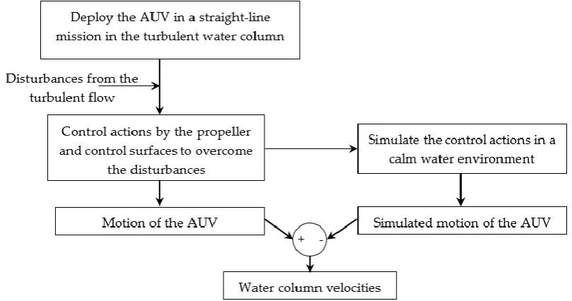
observed vehicle motions. As given in Equation (3.1), the difference between the motion responses in the turbulent (i.e., experimental) and calm (i.e., simulated) water flow condition provides a measurement of the water column velocities relative to the ground. ... 74 Figure 3.4 – Inertial and body-fixed frames of reference. The origin of the body-fixed

coordinate system was at the centre of buoyancy of the vehicle (marked by the filled circle). ... 75 Figure 3.5 – Simulation model flowchart. The acceleration vector of the current time-step is

solved using the velocity vector from the previous time-step and commanded propeller RPM while θ, q, r, q, and r are subsequently replaced with the values recorded during field tests. The body-fixed velocity vector was obtained by integrating the acceleration vector with respect to time. ... 78 Figure 3.6 – (a) The vertical velocity of the vehicle observed in the turbulent (experimental)

and calm (simulated) water environments. The difference between the two responses provides the velocity of the water column in the z direction. The comparison between the velocity components of the water column in x, y and z axes (panels (b), (c), and (d), respectively) was calculated using the WVAM method and those obtained from the ADCP measurements smoothed with a moving average filter. ... 83 Figure 3.7 – The variation of the difference between ADCP and WVAM vertical water velocity

magnitudes with the vertical distance from the AUV. ... 86 Figure 4.1 – (a) An AUV descending to a test site in blue water where the bottom track

(20)

to reach the seabed, and (b) DVL is incapable of providing continuous bottom track velocity measurements when travelling over rough bathymetry. ... 92 Figure 4.2 – (a) Omarama Primary School (Lake Ohau, New Zealand) students inspecting the

Gavia, the modular AUV that was utilised to test the WVAM method, (b) the tested configuration of the vehicle, and (c) the body-fixed coordinate system (origin at the centre of buoyancy – marked by the filled ‘O’) showing the ADCP beam geometry. 94 Figure 4.3 – (a) The experimental field site in Tasmania, Australia (inset), (b) the Tamar estuary

with a bi-directional arrow representing the AUV track, and (c) due to the proximity to the open sea and the flow constriction of the river bed, the site exhibited strong tidal currents. ... 95 Figure 4.4 – The water level relative to the Mean Sea Level (MSL) observed on 14 and 15

April, 2015 with the time periods that the AUV runs were conducted indicated by filled diamond markers. ... 95 Figure 4.5 – Panels a, c and e illustrate the variations of the water column velocity components

(i.e., velocities in x, y and z directions respectively) with the vertical distance from the AUV. The water column velocities from 0 – 0.5 m are from the WVAM method while the rest of the profile is from the ADCP measurements. The illustrated velocity data were obtained from Run 1 when the AUV was moving with the predominant tidal currents. ... 99 Figure 4.6 – Comparison of the horizontal water velocities obtained from the WVAM method,

stationary ADCP and the AUV fixed ADCP – modified from (Green et al., 2016) . 100 Figure 4.7 – The variations of the WVAM method’s standard errors with the averaged

fluctuations of the vehicle surge speed and, yaw and pitch angles from the prescribed values. The water column velocity components in x, y and z directions correspond with the surge speed, yaw angle and pitch angle respectively. ... 102 Figure 5.1 – Omarama Primary School students inspecting the utilised Gavia AUV.

Configuration of the vehicle – (A) Nose Cone Module, (B) Battery Module, (C) Geoswath Module, (D) ADCP/DVL Module, (E) INS Module, (F) Control Module and (G) Propulsion Module. ... 112 Figure 5.2 –Tamar estuary experimental field site near the Batman Bridge was located in

(21)

Figure 5.3 – Flowchart of the proposed technique of estimating the absolute position of the AUV using unaided INS acceleration measurements and AUV control commands. wrt stands for ‘with respect to’. ... 117 Figure 5.4 – RMS of the vehicle horizontal (i.e., the magnitude of u and v) velocity prediction

difference of each method compared to the solution from DVL bottom-track aided INS. The ‘OR filtered model-aided’ results represent the outcome from Block (3) of Figure 5.3 while the ‘Proposed technique’ results are the final localisation solution from Block (5). ... 123 Figure 5.5 – comparison of the horizontal velocities from the proposed technique with other

aiding mechanisms for (a) Mission 6 and (b) Mission 5. Velocity calculation from the OR filtered model-aided INS as well as the final estimate are given. ... 124 Figure 5.6 – comparison of horizontal water column velocities (i.e., the magnitude of u_water

and water

v ) from the proposed flow profile smoother against the ADCP measurements for (a) Mission 5 and (b) Mission 4. ... 127 Figure 5.7 – the vehicle localisation solutions of (a) Mission 5 and (b) Mission 6, in a local

coordinate system... 128 Figure 5.8 – the localisation errors at the end of each mission as a percentage of the distance

(22)

List of Tables

Table 2.1 – Specifications of Gavia AUV sensor packages. CEP for Circular Error Probable and TRMS for Time Mean Root Squared. ... 40 Table 2.2 – y(t), H(t) and Θ(t) vectors of Equations (2.12) and (2.16) for x, y and z directions. 49

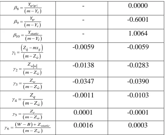
Table 2.3 – Numerical values of the Gavia AUV’s baseline parameters determined from RLS and PEM techniques using ID Manoeuvres 1 and 2. Note that the values of the parameters are not pure hydrodynamic, hydrostatic and mass coefficients as the environmental and external forces are overlayed within them. ... 53 Table 2.4 – Accuracies of the vehicle velocity predictions from the four baseline models (i.e.,

models identified with RLS and PEM techniques, with each technique processed twice utilising ID Manoeuvres 1 and 2) compared to velocity measurements from the DVL aided INS. ... 57 Table 2.5 – Numerical values of the Gavia AUV’s baseline model (i.e., from RLS method with

ID Manoeuvre 1) parameters and those of the model calibrated for Lake Ohau. ... 59 Table 2.6 – The variation of the averaged difference between the actual and simulated

accelerations with the forgetting factor for Lake Trevallyn and Ohau runs. ... 63 Table 3.1 – The 6-DOF notation system. ... 73 Table 3.2 – y(t), H(t) and Θ(t) vectors of Equation (11) for x, y, and z directions. ... 79

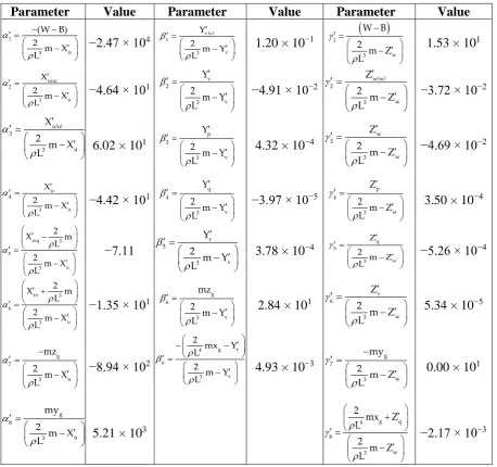
Table 3.3 – Values of the parameters in Equations (3.8) – (3.10) ... 80 Table 3.4 – Uncertainty margin of the WVAM method was determined by adding the individual

error components of each step. ... 85 Table 4.1 – Standard errors of the WVAM method in comparison to the ADCP measurements,

and the associated averaged deviations of the yaw angle, pitch angle and surge speed. ... 101 Table 5.1 – Specifications of Gavia AUV sensor packages. “CEP” for Circular Error Probable

and “RMS” for Root Mean Squared. ... 113 Table 5.2 – Each mission’s descent depth, time taken for the descent and the average of the

(23)

Abbreviations

2D Two Dimensional

3D Three dimensional

3-DOF Three Degree-of-Freedom

6-DOF Six Degree-of-Freedom

ADCP Acoustic Doppler current profiler

ADV Acoustic Doppler Velocimeter

AMC Australian Maritime College

AUV Autonomous Underwater Vehicle

BSLRSM Baseline Reynolds Stress Model

CFD Computational Fluid Dynamics

DVL Doppler Velocity Log

EFD Experimental Fluid Dynamics

GPS Global Positioning System

HPMM Horizontal Planer Motion Mechanism

IMU Inertial Measurement Unit

INS Inertial Navigation System

LBL Long Base Line

MATLAB Matrix Laboratory

MOOS-IvP Mission Oriented Operating Suite – Interval Programming

OR Outlier Rejection

PEM Prediction Error Method

RANS Reynolds Averaged Navier-Stokes

RLS Recursive Least Squares

RMS Root Mean Square

ROV Remotely operated vehicle

RPM Revolutions per Minute

SNAME Society of Naval Architects and Marine Engineers SSTCC Shear Stress Transport with Curvature Correction

(24)

Chapter 1: Thesis Introduction

Introduction

Interest in Autonomous Underwater Vehicles (AUVs) is growing for a wide range of scientific, commercial and military applications due their unique capabilities over surface vessels, and manned and tethered underwater vehicles (Stutters et al., 2008). Although the inception of AUV engineering occurred over a half-century ago, their systems are continuously improving to achieve better performance over a wide range of conditions (Griffiths, 2002). One of the major challenges is AUV localisation, which is complicated by wavelength attenuation of electromagnetic waves in water. This effectively limits radio communications and Global Positioning System (GPS) based localisation to surface operations. Furthermore, the high nonlinearity of the hydrodynamic forces and moments, and the unpredictability of the operating environmental conditions have added to the complexity of AUV manoeuvres and operations.

1.1.1. AUV localisation

Vehicle localisation is the foremost important element of the overall AUV autonomy. It is especially critical to accurately recognise the current position of the vehicle in three dimensional (3D) space for navigation (i.e., point to point guidance of the vehicle) as well as for motion control. Inaccurate localisation could result in the vehicle travelling away from the pre-planned mission route while assuming it is on the correct track, whereby resulting in an incorrectly geo-located dataset and a compromised mission. In the most severe examples of this, mission failure could result leading to a potentially damaged or lost AUV.

(25)

dedicated supporting surface vessel shadowing the AUV for the entire duration of its mission, which is a major disadvantage.

Inertial Navigation System (INS) is one of the most commonly used methods for AUV localisation and navigation. The accelerometers and gyroscopic sensors of the Inertial Measurement Unit (IMU) within the INS measure the linear accelerations and angular rates of the AUV relative to the inertial space (Jalving et al., 2004). Subsequently, the measurements are integrated to determine the velocity, attitude and position of the vehicle. IMU measurements have uncertainties due to inherent errors of its sensors. Due to integration of these uncertainties, an unbounded drift will be accumulated with time in the position and velocity solutions unless true position and/or velocity measurements of the AUV are fed back into the INS position estimate through the use of a predictor-corrector model such as a Kalman filter (Medagoda et al., 2010). The vehicle velocity measurements from a bottom-tracking Doppler Velocity Log (DVL) are commonly used to aid the INS localisation solution in order to avoid the position drift.

1.1.2. Problem definition

(26)

[image:26.595.72.525.74.322.2]

Figure 1.1 – An AUV descends to a test site in blue water where the altitude is larger than the maximum range of the DVL.

The traditional solution used by most currently operating AUVs is to track and measure the velocity of the vehicle relative to the water column; i.e., DVL water-track aided INS. This could provide a reasonably accurate localisation solution when the AUV is operating in environments with small underwater currents. However, the DVL water-track mode is unable to measure the velocity of the water column relative to the ground; therefore, the motion of the water column is often neglected. For this reason, the water-track mode of vehicles is prone to the velocity and position drifts due to the unaccounted movements of the water column in high energy environments with large underwater currents.

(27)

1.1.3. Model-aided INS localisation

The velocity of an AUV can be approximated with a dynamic motion response predicting mathematical model that represents the mass, hydrostatics and hydrodynamic properties of the AUV; i.e., known as a model-aided INS. One of the major advantages of model-aided localisation is that it does not require additional sensors beyond a typical AUV navigational payload and could be simply established with a modification to vehicle firmware. The velocity response predicting capability of such models depends on the accuracy of the parameters representing vehicle characteristics that typically vary with the vehicle configuration and ballast condition. However, previous model-aided INS systems were developed only for a given vehicle setting (Hegrenaes and Hallingstad, 2011, Hegrenaes et al., 2008, Jayasiri et al., 2016, Jayasiri et al., 2014, Yan et al., 2012). Commercial and scientific AUVs often change the configuration of the vehicle due to the addition and removal of payload sensors (Trembanis et al., 2012, Walker et al., 2013). Furthermore, the ballast condition of the AUV will vary with the salinity level of the operational environment. It is hypothesised in this work that a baseline mathematical model with parameters representing a particular vehicle setting may not adequately predict the motion of the vehicle with a different configuration.

Parameters within conventional AUV mathematical models represent the hydrodynamic, hydrostatic and mass properties of an AUV operating in calm water environments. That is, the model is unable to predict the external forces and moments acting on the vehicle such as those due to underwater currents and complex flow conditions (Randeni et al., 2015a). Therefore, the vehicle velocities predicted by a model are not absolute, but relative to the water column; i.e., equivalent to the velocities obtained from DVL water-tracking mode. In order to obtain the vehicle velocity relative to the ground, the motion of the water column needs to be compensated with the water column velocity measurements or predictions.

(28)

accurate due to erroneous INS velocity measurements; since an outlier filtering technique is not utilised in this work. Furthermore, both of these techniques are not readily transferable to a different configuration of the AUV unless the parameter identification procedure is repeated. Finally, their performances were not evaluated for varying environmental conditions.

1.1.4. Objectives and research question

This project aims to improve the localisation accuracy of AUVs operating in low as well as high energy environments when direct DVL aiding is unavailable. An improved model-aided INS localisation technique is introduced by developing the dynamic motion response predicting mathematical model that can be field calibrated for different environmental conditions and vehicle configurations. The model-aided INS localisation technique is complimented with a novel, non-acoustic water column velocity estimation method, in order to counteract the position drift due to sea currents. Combining all of these elements, this project aims to resolve the following research question:

“How can INS localisation accuracy of an AUV operating without DVL bottom-track be

improved for both low and high energy environments?”

Novel techniques established in this project were tested and validated with field experimental data from a Gavia class AUV.

Methodology

The methodology utilised to solve the research question of this project could be broken down into four main phases:

Phase 1: Conducting a study on existing AUV localisation techniques, focusing on previous work carried out to improve the INS localisation performance when DVL aiding is unavailable.

Phase 2: Establishing a methodology to determine an improved AUV motion response predicting mathematical model. This process involved:

(29)

 Development of a model calibration method to field calibrate the baseline model for the current operating environment and vehicle configuration.

Phase 3: Developing a non-acoustic method to estimate the water column velocity components of a high energy environment using AUV motion response (referred to as the ‘WVAM method’), and carrying out the following further evaluation:

 Investigation of the performance of the WVAM method as a function of the turbulence levels of the environment to verify whether the technique is able to predict underwater currents in a blue water environment;

 Examination of the feasibility of the WVAM method to be incorporated with a model-aided INS localisation solution for error counteraction; and,

 Upgrading the WVAM method to determine the water column velocity profile relative to the ground along the descend path of an AUV diving from the surface to the seabed.

Phase 4: Combining the model-aided INS localisation solutions with the WVAM method to improve the localisation accuracy of an AUV descending in blue water without DVL bottom-track.

Novel aspects

This project has provided original contributions to the state-of-art AUV technology in four main areas. The first is the methodology to determine an improved model-aided INS localisation technique that can be field calibrated for different environmental conditions and vehicle configurations. Previous studies have identified mathematical models for AUVs; however, they are limited for a given environmental setting and vehicle configuration (Hong et al., 2013, Marco et al., 2005, Yan et al., 2014). The novelty of this work is that the baseline model identified using complex identification manoeuvres conducted in a calm water environment can be calibrated to diverse operational environments and vehicle settings, online or offline, using the motion response data from a simple mission.

(30)

are usually unknown based on traditional methods. Previously, Hayes and Morison (2002) introduced a non-acoustic technique to determine the turbulent vertical water velocities, and fluxes of heat and salt by applying a Kalman filter to the AUV motion data. However, it cannot be readily adopted for commercial AUVs due to the modelling complexity and the requirement of the typically unavailable vehicle control law algorithm. Furthermore, this method was limited to the vertical water velocity, while the WVAM method estimates the water velocity components in the x, y, and z directions. Estimating horizontal water column velocities in proximity to the AUV (i.e., the water column velocities at the same depth as the vehicle is) is important for vehicle navigation and control system optimisation, and to fill the blanking distance gap within a water column velocity profile, which is important for flow field characterisation for environmental studies.

The third original contribution of this project is the technique introduced to determine the water column velocity profile relative to the bottom along the decent path when DVL bottom-track is unavailable, and utilising it to counteract the localisation error of an AUV diving in blue water. This technique included a novel Outlier Rejection (OR) filter that removes outliers present within the INS measurements, and a flow profile smoothening algorithm that applies a forward and backward correction, and a flow variation smoother to the water column velocity profile.

(31)

Outline of thesis

This thesis follows a “chapterised thesis” structure, where Chapters 2 to 6 and Appendix A are comprised of scientific papers. The outline of the thesis structure is given below.

Chapter 1: Thesis introduction

Chapter 1 is the preface of this thesis that details the motives for the project, providing necessary background knowledge on AUVs and conventional AUV localisation techniques to date. Subsequently, the project objectives, methodology and the novel outcomes are defined. Chapter 1 also outlines the structure of the thesis, linking together the succeeding chapters that are comprised with academic papers.

Chapter 2: Replicating the motion response of an AUV for dynamic environments

(published in the Nonlinear Dynamics journal)

Chapter 2 is motivated by the requirement of a mathematical model that can predict the motion response of an AUV based on its control commands, regardless of the operational environment. RLS and PEM based system identification algorithms are presented to determine the linear and nonlinear parameters of an AUV motion response predicting mathematical model. A baseline mathematical model that represents the dynamics of a Gavia class AUV in a calm water environment is developed. A novel technique is introduced to calibrate the parameters within the baseline model to provide the motion response in different environmental conditions by conducting a calibration mission in the new environment. These models are used to develop an improved model-aided localisation system for AUVs operating without DVL bottom-track in low energy environments.

Chapter 3: WVAM method – a non-acoustic technique to determine the velocity

components of the water column (published in the Journal of Marine Science and

Engineering)

(32)

Chapter 4: Feasibility of WVAM method for AUV localisation error counteraction

(published in the Marine Technology Society Journal)

Chapter 4 further compliments the WVAM method by analysing its feasibility to be incorporated with a model-aided INS localisation system. The study investigates and analyses the performance of the WVAM method as a function of the turbulence level of the environment by testing the method in an estuary that exhibits strong tidal currents (around 2.5 m s-1_{). The}

performance of the WVAM method was compared with the vehicle on-board as well as stationary ADCPs in different water column conditions. This chapter discusses the necessary improvements required to incorporate the WVAM method within a model-aided INS.

Chapter 5: Counteracting AUV localisation error when operating beyond the range of

bottom-tracking sonar (submitted for publication in the IEEE Journal of Oceanic

Engineering)

Chapter 5 combines the work developed in previous chapters and presents an AUV localisation technique based on a mathematical model-aided INS for blue water operations conducted in high energy environments with strong non-uniform currents without DVL bottom-track. Inputs to the algorithm are vehicle control commands and unaided acceleration measurements from the INS. An Outlier Rejection (OR) filter is introduced to remove the outliers present within INS acceleration measurements prior to the data fusion with baseline model predicted velocities. The velocity profile of the water column relative to the ground along the descent path of the AUV is determined to avoid localisation drift resulting from underwater currents. The water column velocity profile is obtained with a flow velocity profile smoothing algorithm, which is an extension of the WVAM method.

The proposed technique is tested and validated for diving missions conducted at different water column conditions using a Gavia-class AUV. Its performance was evaluated by comparing with the localisation solutions from DVL bottom-track aided, DVL water-track aided, model-aided, and unaided INS systems.

Chapter 6: Summary, conclusions and future work

(33)

Appendix A: WVAM method in high energy environments (published in the Proceedings

of the ‘MTS/IEEE Oceans 2015’)

The purpose of the WVAM method is to predict the underwater currents acting on the vehicle in order to counteract the drift in the model-aided INS localisation solution of an AUV that operates in blue water. Water column velocity conditions in blue water environments are highly variable. Therefore, Appendix B investigates and analyses the performance of the WVAM method as a function of the turbulence level of the environment by testing the method in an estuary that exhibits strong tidal currents (around 2.5 m s-1_{). The uncertainty of this}

method at different water column conditions was computed by comparing the velocity measurements from the WVAM method with those obtained from the AUV mounted ADCP.

Appendix B: Least squares based system identification algorithm to obtain a

mathematical model of an AUV (published in the proceedings of the Third Vietnam

Conference on Control and Automation)

Appendix B presents a secondary system identification technique based on Least Squares optimisation algorithm to determine the mathematical model of a Gavia class AUV. The purpose of the model is to accurately predict the system response over time starting from initial conditions. Appendix B is comprised of an article that provides an in detail explanation of the Least Squares optimisation algorithm as well as the formation of dynamic equations of motion.

Appendix C: Numerical Investigation of the Hydrodynamic Interaction between Two

Underwater Bodies in Relative Motion – A secondary CFD based approach of

determining the hydrodynamic coefficients of an AUV (published in the Applied Ocean

Research journal)

(34)

Chapter 2: Replicating the motion response of an

AUV for dynamic environments

This chapter is based on the journal article ‘Parameter identification of a nonlinear model: replicating the motion response of an autonomous underwater vehicle for dynamic environments’ that is published in the journal ‘Nonlinear Dynamics’. The citation for the article is:

(35)

Abstract

(36)

Introduction

Autonomous Underwater Vehicles (AUVs) have evolved as specialised tools for challenging commercial, scientific, and military underwater applications such as subsea inspections (Mcleod et al., 2012), characterisation of the midwater column (Curtin et al., 1993) and security exercises in unstructured environments (Paull et al., 2014). Despite the developments of AUVs reaching back to the 1970s, the navigation and control subsystems of AUVs are continuously undergoing improvements (Hegrenaes and Berglund, 2009). In particular, one of the main challenges is accurate localisation and navigation in blue water (i.e., operating in regions out of range of bottom-track aided navigation), and to achieve the dynamic control stability of the vehicle that determines the data quality of AUV surveys (Paull et al., 2014).

Inertial Navigation Systems (INS) are one of the key methods to localise and navigate AUVs. An INS determines the position, velocity and orientation of the vehicle using data from Inertial Measurement Units (IMUs) relative to inertial space. Due to inherent errors, the INS localisation solution in its free inertial mode (i.e., unaided INS) rapidly drifts unless it is externally aided with vehicle’s speed over the ground measurements from a bottom tracking Doppler Velocity Log (DVL) (Jalving et al., 2003, Medagoda et al., 2010). When DVL aiding is intermittently or completely unavailable (for example, due to instrument noise or as a result of the vehicle-to-seabed-distance being larger than the transmission range of acoustic frequency associated with the DVL), the vehicle velocities can be approximated with a mathematical model that characterises the hydrostatic and hydrodynamic properties of the AUV; i.e., a model-aided INS (Hegrenaes et al., 2008, Jayasiri et al., 2016). Although the localisation solution from a model-aided INS is not as accurate as a DVL aided INS, its accuracy is better than the unaided INS and the water-track mode of the DVL aided INS (Hegrenaes and Hallingstad, 2011).

(37)

presence of high currents (Randeni et al., 2016). An improvement in the velocity prediction is essential to increase the AUV localisation accuracy from a model-aided INS.

A dynamically stable control system is essential for AUVs to undertake challenging tasks in complex flow conditions in high turbulent environments (Randeni et al., 2015a), in close proximity to the seabed (Ananthakrishnan, 1998), or to other moving underwater vehicles (Randeni et al., 2015b) and near the free surface (Polis et al., 2013). AUV control systems can be pre-optimised using a mathematical model that represents the dynamics of an AUV in its anticipated operating water column. With the availability of a mathematical model that updates in real time to characterise the operational environment, the control system optimisation can be conducted in real time or near real time (Hong et al., 2013).

Mathematical models can additionally be used to accurately predict the vehicle motion response which, in turn, is crucial for several other applications. For example, the velocity components of a turbulent water column can be determined through a non-acoustic technique using the AUV motion response; as previously described by the authors as the WVAM method in Randeni et al. (2015a). The WVAM method uses a mathematical model to calculate the flow velocities by comparing the actual motion response of the vehicle with the simulated response from a calm water based mathematical model. In addition, AUV simulators are used by vehicle developers and operators to test their mission plans and software modifications as well as to conduct trainings prior to field trials (Song et al., 2003). Such simulators need a mathematical model with precise representation of the vehicle characteristics to accurately simulate the dynamic motion response of the AUV.

(38)

This paper presents a system identification algorithm to determine the linear and nonlinear parameters of an AUV mathematical model utilising the Recursive Least Squares (RLS) and the Prediction Error Method (PEM) optimisation techniques. The developed model accounts for the coupling effects influencing the surge, sway and heave velocities of the vehicle as well as the environmental and external forces. Utilising the model identification algorithms, the parameters of a Gavia class AUV mathematical model were estimated using motion response data from a complex identification manoeuvre conducted in a small, relatively calm lake (i.e. minimal surface mixing. A comparison is made between RLS and PEM, and the dependency of the parameters on the utilised dataset is also investigated. The identified model parameters are able to predict the motion response of the AUV in calm water condition and is referred to as the ‘baseline’ mathematical model hereafter. A novel technique is presented to field calibrate the baseline mathematical model to predict the vehicle motion response in diverse operational environments. The model calibration algorithm was extended to determine the AUV mathematical model in real time, processing a limited preceding data window for future goals such as real time control system optimisation. The following sections of this paper provide an overview of the field experimental setup (including the details of the utilised Gavia AUV and test site details), theory and justification of AUV dynamic modelling equations utilised in this study, and a brief description of the RLS and PEM techniques and the model simulation method. Baseline model estimation procedure and model calibration method are then explained together with a performance analysis. Finally, the real time model calibration is discussed, followed by a summary on possible future developments and conclusions.

Field experimental setup

2.2.1. Instrumentation

(39)

a three bladed ducted propeller system with four individually functioning control surfaces arranged in an ‘X’ configuration.

Figure 2.1 – Body-fixed frame of reference and the configuration of the utilised Gavia AUV. The origin is located at the centre of buoyancy of the vehicle. The vehicle had a length of 2.7 m, a

diameter of 0.2 m, and a dry weight in air of approximately 70 kg

The DVL aided Kearfott T24 INS measured the accelerations in Six-Degree-of-Freedom (6-DOF) and orientation, to make estimates of the AUV’s velocities and position. The heading and pitch angles of the vehicle were measured by the gyroscopic sensors, while the accelerations were determined through the use of accelerometers within the INS unit. The

(40)

Table 2.1 – Specifications of Gavia AUV sensor packages. CEP for Circular Error Probable and TRMS for Time Mean Root Squared.

Sensor package Measurements Measurement accuracy

DVL bottom-track/GPS aided INS

Heading angle ±0.010° (RMS) Pitch angle ±0.005° (RMS)

Position estimate 0.1% of the distance travelled (CEP) Velocity estimate

(DVL aided)

0.001 m s-1 (RMS)

Velocity estimate (GPS aided)

0.05 m s-1 (RMS)

DVL water-track aided INS

Position estimate 1852 m per 8 hours (TRMS) 4.02% of the distance travelled*

Velocity estimate 0.3 m s-1_(RMS)

1200 kHz Teledyne RDI DVL

Bottom tracking AUV velocity

±0.001 m s-1 (RMS) or 0.2% of the velocity

Maximum bottom tracking range

30 m

Keller Series 33Xe pressure sensor

Vehicle depth 0.1% of the depth

*_{derived from the 1 nm per 8 hours uncertainty value for comparison, assuming an AUV}

forward speed of 1.6 m s-1

2.2.2. Test site and experimental runs

The objectives of the field studies were to develop and to validate the parameter identification and calibration algorithms for different environments. Field studies were conducted in two locations: Lake Trevallyn in Tasmania, Australia (Figure 2.2a) and in Lake Ohau, South Island, New Zealand (Figure 2.2b).

(41)

[image:41.595.79.503.119.549.2]

respectively. Due to these very small flow velocities, Lake Trevallyn can be classified as a calm water environment.

Figure 2.2 – AUV field deployments were conducted (a) in Lake Trevallyn, Tasmania, Australia and (b) Lake Ohau, South Island, New Zealand. Parameters of the mathematical model were

determined from the manoeuvres conducted in Lake Trevallyn. The estimated models were verified with the vehicle motion response data from AUV deployments in Lake Ohau - eight AUV runs were conducted in a lawn-mover pattern (inset). (c) Bathymetry along the AUV Run

1, conducted in Lake Ohau, New Zealand

(42)

were around 0.15 m s-1 (Cossu et al., 2015). The test site at Lake Ohau had highly variable bathymetry; i.e., rough in proximity of the delta front as well as relatively flat lake floor in deeper parts of the lake (Figure 2.2c). For constant altitude AUV missions, the vehicle experienced highly fluctuating pitch angles (i.e., over ±10°) when flying above the region of variable bathymetry (i.e., up to 200 m from the starting position), while angles of less than ±2° were maintained above the flat terrain. For these reasons, the test site was decided to be a suitable stage to test the AUV mathematical models for different vehicle responses.

(43)

In Lake Ohau, a lawn-mower pattern mission with eight transect lines was conducted. Each straight line run was carried out over the diverse bathymetry (i.e., the water depth was varying from around 50 – 60 m) maintaining a constant altitude of 8 m above the seabed. The first four lines (runs 1-4) of the lawn-mower pattern were used to calibrate the baseline model for the Lake Ohau water column condition utilising the model calibration method introduced in this work. The performance improvement of the calibrated model compared to the baseline model was analysed by testing the model with the last four lines (runs 5-8). Therefore, both calibration and performance analysis runs included smooth as well as rough bathymetric conditions.

Validation of the real time model estimation algorithm was conducted in Trevallyn as well as Ohau sites in order to establish its robustness in different field conditions. During all field tests, the vehicle altitude was within the range of the DVL acoustic beams, continuously aiding the INS solution. Hence, the motion response measurements used for model validations were maintained within the DVL aided INS uncertainty limits as given in Table 2.1.

Figure 2.3 – Three types of manoeuvres were conducted in Lake Trevallyn site; i.e., zig-zag manoeuvres in yaw plane (section shaded in dark grey) and pitch plane (shaded in light grey),

and step changes of propeller speed from 450RPM to 975RPM (no shading)

Dynamic modelling of the AUV

2.3.1. Notation

(44)

2.3.2. AUV mathematical model

Manoeuvring equations of motion derived by considering the rigid-body kinetics, hydrodynamics, hydrostatics, environmental and other external forces acting on the AUV are generally used for vehicle modelling (Fossen, 2011, Newman, 1977, Fossen, 2002). In the work presented here, we used a basic mathematical model given in Equation (2.1) as specified for underwater vehicles by Fossen (2002); however, the hydrodynamic, environmental and control forces were modelled using a new mathematical model. One of the key advantages of this work is that the utilised mathematical model can be applied for any torpedo shaped AUV of any configuration.

 

RB RB A A external

M ν C+ ν ν M ν C ν ν D ν ν g η+ + + + = +τ τ (2.1)

where, MRB and MA are the rigid body and added mass system inertia matrices, CRB and

CA are the rigid body and added mass Coriolis-centripetal matrices, D is the hydrodynamic

damping matrix, g η

 

is the restoring gravitational/buoyancy force matrix, τ is the vector of propulsion and control surface forces, and τexternalrepresents the vector of environmental and

 Z (2.4)

where the term m is the mass of the vehicle and xg, yg and zg represent the position of the

(45)

Xprop is the thrust produced by the propeller. The right-hand side of these equations (i.e.,



X,



Yand



Z) represent the summation of hydrodynamic damping, and environmental and external forces.

2.3.4. Hydrodynamic damping and external & environmental forces

Hydrodynamic damping of underwater vehicles is a result of several factors including: (1) the linear skin friction due to laminar boundary layer dynamics, (2) the nonlinear skin friction due to turbulent boundary layer dynamics, (3) the viscous damping force due to vortex shedding, (4) the form drag due to pressure variation across the body, and (5) the hydrodynamic lift forces due to cross flow drag and circulation of water around the hull (Fossen, 2011). Therefore, linear as well as higher order damping terms and relevant cross flow coupling terms are required to accurately model the flow around the vehicle (Abkowitz, 1964, Fossen, 2011). It is also important to model the vehicle dynamics with a minimum number of parameters because if the number of unknown parameters present in a model is large, the accuracy of the parameter estimation reduces (Ljung, 1999).

When using a mathematical model, an accurate description of environmental and external forces is required for calibration. In marine vehicle modelling, it is common to assume the principle of superposition when considering these highly nonlinear forces (Fossen, 2011). This principle suggests that the generalised environmental and external forces are added to the right-hand side of Equation (2.1); i.e., τexternal.

2.3.4.1. Forces in x direction

In the current work, the hydrodynamic damping along the x direction is modelled using Equation (2.5).

3

| |

XXuuuu X u uu u X uu X wqwq X vrvr X     | | X Xstatic

 (2.5)

where the notation of the hydrodynamic coefficients follow SNAME (1952). For example, Xu is the derivative of the surge force (X) with respect to the surge speed (u); i.e.,

u

X

  

X u

. Xψ|ψ| and Xψ are the surge force coefficients due to underwater currents. Xstatic

stands for variable independent static external forces along x direction.

This equation is comprised of damping terms up to the third order (i.e., Xu, Xu|u|and Xuuu);

(46)

the forward speed of the AUV resulting from heading and pitch variations. The external forces due to underwater currents depend on the heading of the vehicle. For example, if a steady underwater current is flowing from North to South, the external current force component acting on the vehicle when travelling with a heading angle of 0° would be different to a heading angle of 60°. Fossen (2011) models the forces due to underwater currents as a function of angle of attack of the AUV with the flow direction, which is also a function of the vehicle heading angle. Hence, in this work, external forces along the x direction due to current are modelled as functions of up to the second order of the vehicle heading (i.e., Xψ|ψ| and Xψ). Other

environmental and external forces (i.e., direction independent) acting along the x direction are assumed to be superimposed within the damping hydrodynamic parameters. This offers the ability to capture the external forces as functions of all the previously stated variables for different environmental conditions, maximising the accuracy of model calibration and minimising the number of data points required for the convergence. However, this has a disadvantage of not being able to obtain values for the pure hydrodynamic derivatives as environmental and external forces are incorporated in them. Any uncaptured steady external forces are included in the model as a variable independent constant Xstatic.

2.3.4.2. Forces in y direction

Similarly, the hydrodynamic damping forces and environmental/external forces acting along the y direction are modelled using Equation (2.6).

| |

YY v vv v Y v Y q Y r Y p Yv  q  r  p       | | Y Ystatic

 (2.6)

Nonlinear hydrodynamic damping along y direction was limited to the second order of the sway velocity (i.e., Yv and Yv|v|). The Gavia AUV is asymmetric about the x-y and y-z planes.

Therefore, as the vehicle presents an angle of yaw to the flow (i.e., as the vehicle changes its horizontal heading angle), the AUV will start to roll and pitch, resulting in a change in the vehicle operating depth as the control system responds. Due to the asymmetry of the vehicle, this will occur in all directions. Therefore, the linear cross-coupled drag components due to roll, pitch and yaw motions (i.e., Yp, Yq and Yr) were also included in Equation (2.6). Similar to

the surge model, the sway force due to steady underwater currents is modelled as functions of up to the second order of the vehicle heading (i.e., Yψ|ψ| and Yψ). The direction independent

(47)

2.3.4.3. Forces in z direction

Equation (2.7) describes the hydrodynamic damping and environmental/external force along the heave direction.

ZZ_{w w}w wZ w Z q Z r_w  _q  _r Z_static

 (2.7)

Similar to the sway force component, the nonlinear hydrodynamic damping in the z direction was limited to the second order of the heave velocity (i.e., Zw and Zw|w|). The

cross-coupled damping terms due to pitch and yaw motions (i.e., Zq and Zr) were also included. The

environmental/external forces acting along the heave direction were also assumed to be superimposed within the modelled hydrodynamic damping parameters. Uncaptured steady external forces are incorporated as a variable independent constant Zstatic, which also represents

any variations in the ballast condition from the baseline model. The heading direction dependent underwater currents along the vertical direction are neglected.

2.3.5. Final dynamic equations of motion and control forces

Equations (2.2) and (2.5) are combined and rearranged to determine the surge acceleration as shown in Equation (2.8).







  

3

| |

1

[ sin

| | ]

g g uuu u u

u

u wq vr static prop

u my r mz q W B X u X u u

m X

X u X wq X vr X_{ } X_ X X

       



        

(2.8)

where, Xprop is the thrust produced by the propeller that is given by XnRPM2. RPM is

the vehicle’s propeller revolutions per minute and X_nis the thrust coefficient, which is 95×10 -6_{for the Gavia AUV according to the estimation by Thorgilsson (2006). The thrust coefficient}

is only valid for the propeller speed range from 450 RPM to 975 RPM.

Improving the localisation accuracy of AUVs operating in highly variable environmental conditions