Feature Extraction Methods for Character Recognition

(1)

Theses

Thesis/Dissertation Collections

2004

Feature Extraction Methods for Character

Recognition

Roman V. Yampolskiy

Follow this and additional works at:

http://scholarworks.rit.edu/theses

This Thesis is brought to you for free and open access by the Thesis/Dissertation Collections at RIT Scholar Works. It has been accepted for inclusion

in Theses by an authorized administrator of RIT Scholar Works. For more information, please contact

[email protected].

Recommended Citation

(2)

Feature Extraction Methods for

Character Recognition.

Department

ofComputer

Science

Master's Thesis

by

Roman

V.

Yampolskiy

Department

of

Computer Science

Rochester

Institute

of

Technology

Rochester,

NY,

USA

[email protected]

(3)

Feature Extraction Methods for Character Recognition

By

Roman V. Yampolskiy

A Thesis

Submitted to the Faculty of B. Thomas Golisano College of

Computing and Information Sciences in Partial Fulfillment of the

Requirements for the Degree of Master of Science in Computer

Science

Approved by:

Professor Leonid Reznik, Chair

Date

Approved by:

Professor Peter G. Anderson, Reader

Approved by:

________________________________

'_'_M~~~~~1

Professor Roger S. Gaborski, Observer

Date

(4)

Thesis Reproduction

Permission Statement

Permission granted

Title of thesis: Feature Extraction Methods for Character Recognition.

I, Roman V Yampolskiy, hereby grant permission to the RIT Library

of the Rochester Institute of Technology to reproduce my thesis in whole or

in part. Any reproduction will not be for commercial use or profit

.

Date: May 10, 2004

(5)

(6)

Page

5

conducted.

Optimal

parameters

for

learning

rate,

spread, momentum,

num

ber

of

layers,

number of nodes and number of epochs

for

this

particular

application were

found.

Radial

Basis

Function Network

was chosen as

the

superior

classifier,

both in

terms

of

its

speed and accuracy.

A

novel

feature

extraction

method,

called

Fuzzy Zoning,

was

developed.

Fuzzy

Zoning

's

main competition was with other

zoning

approaches and un

like

all of

them,

it

was

designed

to

counteract

the

problem of

sharp

zone

borders

by

allowing

a single pixel

to

contribute

to

multiple zones at

the

same

time.

Fuzzy Zoning

was analyzed and

included in

the

classification with other

zoning

based

features.

Based

on experiments and

test results,

all

feature

extraction methods were

ordered against

their

accuracy.

As

this

ordering didn't

consider

time

com

plexity

required of

the

classifier

to

work with a particular

feature,

the

size of

the

feature

vectors was

taken

into

consideration

for

comparison purposes.

A

new metric was

developed,

which was called

Normalized

Accuracy

Mea

sure.

Unlike

a simple

accuracy,

this

metric considers

time

complexity

of

feature

classification.

This

approach allows

optimizing the total

character

recognition

operation,

which

includes both

feature

extraction and classifica

tion.

All feature

extraction methodswere compared and ordered against

the

developed Normalized

Accuracy

Measure

metric.

Keywords:

Feature

Extraction,

Optical Character

Recognition,

Nor

malized

Accuracy

Measure,

Fuzzy Zoning, Invariance, Handwritten,

Clas

sifier,

Off-line

features,

Pattern

Recognition,

Neural

Network,

Radial

Basis

Function

Network,

Multiple Layer Perceptron

Network, Handprinted,

Projec

tion

Histogram, N-tuple,

Hough

Transform,

Chain

Code

Transform,

Gabor

Filter,

Feature

Points, Strokes,

Character

Profiles,

Graph

Description,

Char

acteristic

Loci,

Shadow

Code,

Template

Matching, Zoning,

Angular

Parti

tions,

Radial

Coding,

Concentric

Circles,

Tracks

and

Sectors, Ring

Projec

tion,

Crossing

Method, Moments, Geometric, Central, Transformed,

Gegen-bauer, Legendre, Tchebichef

Krawtchouk,

Zernike, Pseudo-Zernike,

Fourier-Mellon, Wavelets,

Fractal

Encoding,

Fractal

Feature, Structural,

Statistical,

(7)

If

you wish your merit

to

be

known,

acknowledge

that of

other people.

Oriental Proverb

First

and

foremost,

I

would

like

to thank

members of

my

committee:

Dr.

Roger S. Gaborski

who

has

planted

in

me

the

seed of

interest

in

computer

vision

and

I'm

forever

grateful

to

him

for

that.

Among

other

things,

he has

wel

comed

me

into

the

world

of

Matlab

programming,

which

was

essential

for

the

success of

this

research project.

Dr.

Peter

G. Anderson

introduced

me

to the

field

of

pattern

recognition

and

laid

the

foundation

of

knowledge,

which

allowed

me

to

undertake

such

an

interesting

endeavor.

Additionally,

it

was

because

of

his

enthusiasm

that

I

was

able

to

learn

and master

the

art of

L^TgX. I

would

like

to

particularly

thank

my

advisor,

Dr. Leonid

Reznik,

whose

encouragement

and support made

the

process of

working

on

this

thesis

truly

enjoyable.

His

overall

contribution

(8)

Page 7

Special thanks goes to all the people who supported my

efforts: RIT librarians for doing the impossible in trying

to locate seminal papers from the early sixties. CS

de-partment lab personal for letting me print a forest worth

of drafts and sizable final copies of this thesis.

Gradu-ate Program Coordinator Dr. Hans-Peter Bischof and all

the secretarial staff for their help in processing my thesis

continuation requests. My fellow graduate student Dima

N ovikov for his help with Matlab.

On a more personal note, I would like to express my

grati tude to my parents who have always supported and

believed in me. Last but not least, I would like to

con-vey my appreciation to Kira Shvarts, who has helped in

a number of ways including proofreading this thesis.

(9)

Title

1

Signature

Page

2

Thesis Reproduction Permission Statement

3

Abstract

4

Acknowledgements

6

Contents

8

List

of

Figures

13

1

Introduction

25

1.1

Introduction to

Character Recognition

. .

25

1.2

Pattern Recognition

System

. . . .

26

1.2.1

Data

Collection

26

(10)

CONTENTS

Page 9

1.2.3

Feature Extraction

28

1.2.4

Classification

28

1.2.5

Postprocessing

29

2

Feature Extraction Methods

30

2.1

Features Utilized

by

a

Human

Reader

30

2.2

Image

Partitioning

Approaches

32

2.2.1

Zoning,

a.k.a.

Sub-window Pixel Count

32

2.2.2

Fuzzy

Zoning

34

2.2.3

Zoning

-

Gegenbauer Moments

69

(11)

2.4.7

Tchebichef Moments

72

2.4.8

Krawtchouk Moments

76

2.4.9

Zernike Moments

78

2.4.10

Pseudo-Zernike Moments

81

2.4.11

Fourier-Mellon Moments

83

2.5

Structural Approaches

85

2.5.1

Structural Features

85

2.5.2

Feature Points

87

2.5.3

Strokes

89

2.5.4

Character Profiles

92

2.5.5

Graph Description

98

2.5.6

Crossings Method

99

2.6

Transform

Based Approaches

103

2.6.1

The Fourier Transform

. .

103

2.6.2

Gabor

Filter

108

2.6.3

Hough Transform

Ill

2.6.4

Chain Code

120

2.7

Fractal

Based Approaches

128

2.7.1

Fractal

Encoding

128

2.7.2

Fractal Feature

130

2.8

Other

Approaches

132

2.8.1

Characteristic Loci

132

(12)

CONTENTS

Page 11

2.8.3

Shadow Code

140

2.8.4

Template

Matching

.146

3

Classification

Using

Neural

Network

150

3.1

NN

for Pattern Recognition

150

3.1.1

Multiple

Layer Perceptron Network

.... .152

3.1.2

Radial Basis

Function

Network

.153

3.1.3

MLPN

vs

RBFN

. .

153

4

Experiment

and

Program Descriptions

155

4.1

Description

of

Programs

. .

155

4.2

Data

Set Description

158

4.3

Description

of

Experiments

161

4.3.1

Experiment

1:

Optimization

of

MLPN

162

4.3.2

Experiment 2:

Optimization

of

RBFN

165

4.3.3

Experiment 3: Performance

Comparison

165

4.3.4

Conclusions

with respect

to

MLPN

and

RBFN

.

169

5

Summary

of

Results

170

5.1

Taxonomy

of

Features

170

5.2

Summary

of

Results

175

5.3

Normalized

Accuracy

Measure

.... .

179

5.4

More

on

Individual Features

... .

183

(13)

5.4.2

Histogram Based

Approaches

185

5.4.3

Method Of Moments

186

5.4.4

Structural Approaches

187

5.4.5

Transform Based Approaches

188

5.4.6

Fractal Based

Approaches

...

190

5.4.7

Other

Approaches

190

6

Conclusions

192

6.1

Accomplishments

... . .

192

6.1.1

Future

Work

194

7

Appendix A:

Taxonomy

of

Geometric

Features

195

(14)

List

of

Figures

1.1

A

gap

and noise

in

the

character

T

[171]

. . .27

2.1

Bouma's

classification of

letters

[272]

31

2.2

Upper-left:

character

A;

Upper-Right:

Zoning

grid

imposed;

Lower-Left:

binary

zoning

feature;

Lower-Right:

sub-window

pixel counts .

32

2.3

Zoning

on a

gray level image,

(a)

A

4

x

4

grid on a

gray

scale

character,

(b)

The resulting

average

gray

levels for

each zone

[262]

34

2.4

Fuzzy

contribution of pixels

located

in

a corner or

in

a middle

of a pattern

35

2.5

Fuzzy

mask with

linear decrease

in

pixel contribution of

10

percent

for

each concentric square . . .

36

(15)

2.7

Zoning

method with

fuzzy

borders.

Pixel

Px

has

a

fuzzy

mem

bership

value of .25

in

each of

the

four

zones

A, B,

D,

and

E.

P2

has

a .75

membership

value

in

zone

E

and .25

in

zone

F

[262]

38

2.8

Zoning

combined with contour

line

segment counts,

(a)

char

acter subdivided

into 16 equally

sized

zones;

(b)

contour

lines

in

the

upper-right zone

only;

(c)

count ofcontour

lines

for

this

zone.

[262]

39

2.9

(a)

Normalized

digit

4.

(b)

Digit 4

partitioned

into 6x4 boxes.

(c)

pattern of

digit

4

plotted

using

extracted

features

[92].

. .

40

2.10

Zoning

using

a quad

tree

[256]

41

2.11 Left:

Digits

'0',

'3', '6',

and '9' with

16

angular partitions.

Right:

Digit

'3'

with

32

Angular

partitions

[206, 205]

42

2.12

Differences between

the

letters

'M' and 'N'

[260]

43

2.13

Difference in

size of

the two

largest

arcs outside

the

pattern

for

the

letters

'M' and 'N'

[260]

44

2.14

Concentric

circles applied

to

letters

'M' and

'N'

[260]

44

2.15 Normalized

differences

obtained

for

the

letters

'M'

and 'N'

[260].

45

2.16

Concentric

circles applied

to

letter

LE\

shown

in

different

rota

tions

and sizes.

Numbers

in

the

first line indicate

the

number

of

intensity

pixel changes

in

each one of

the

eight circumfer

ences.

Second line

represents

the

normalized

differences

over

(16)

LIST OF FIGURES

Page

15

2.17

A

segmentation scheme with

12

sectors and

3

tracks

[57].

...

47

2.18

Semented

images

of characters

'G'

and

'H'

[57].

. ....

48

2.19 Segmented

image

of

digit

6

[100]

48

2.20 Horizontal

and vertical projection

histograms

for digit five

[262]

51

2.21 2D

reduction

to

ID using

a slit of

light

[180]

51

2.22

Horizontal, Vertical,

Left

diagonal,

and

Right diagonal

projec

tion

histograms

[234]

...

52

2.23 Horizontal

histograms

on a mesh par

titioned

Korean

character

[133]

53

2.24

Horizontal

histograms

of

Marathi

char

acter

[203]

53

2.25 Different

geometric shapes can produce

identical

projection

histograms

[180]

54

2.26

Ring

Extraction

panel

[246]

55

2.27

Ring

projection

[246]

55

2.28

Ring

Projection

associated with accumulation

[246]

57

2.29

Reconstruction

of

the

letter

'E'

by

Legendre

moments.

From

top

to

bottom

row and

left

to

right

in

each row: original

input

image,

reconstructed

image

with

up to

second order moment

through up to twentieth

order moment

[47]

71

2.30

Reconstruction

of

the

letter

'E'

by Tchebichef,

Legendre

and

(17)

2.31

Reconstruction

of

the

Chinese

character

by

higher

order

Tchebichef

and

Legendre

moments with reconstruction error shown

[183].

75

2.32

Reconstruction

of

the

Chinese

character

by

higher

order

Tchebichef

and

Legendre

moments with reconstruction error shown

[183].

75

2.33 Reconstruction

of

the

letter

'E'

by

Tchebichef,

Legendre,

Zernike,

Pseudo-Zernike

and

Krawtchouk

moments of orders

9

through

16,

with reconstruction error shown

[284]

77

2.34

Reconstruction

of

the

letter

'E'

by

Zernike

moments.

From

top

to

bottom

row and

left

to

right

in

each row: original

input im

age,

reconstructed

image

with second order moment

through

up

to twentieth

order moment

[47]

78

2.35 Examples

of

letters

reconstructed with

Zernike

moments

up

to the twelfth

order

[171]

79

2.36

Examples

of

digits

reconstructed with

Zernike

moments

up to

the twelve

order

[136]

79

2.37 Reconstruction

of

the

letter

'E'

by

Pseudo-Zernike

moments.

From

top

to

bottom

row and

left

to

right

in

each row: origi

nal

input

image,

reconstructed

image

with

up to

second order

moment

through

up

to

twentieth

order moment

[47]

82

2.38 Examples

of

letters

reconstructed with

Pseudo-Zernike

mo

ments

up to the twelfth

order

[171]

82

2.39 Reconstruction

of

the

letter

'b'

by

Fourier-Mellon

moments.

(18)

LIST

OF

FIGURES

Page

17

2.40

Reconstruction

of

the

letter

'h'

by

Fourier-Mellon

moments.

Reconstructed

image

with

up to

441

moments

[97]

84

2.41

Digit

six with some of

its

structural

features

shown

85

2.42

Decision

tree

for

numerical

images

[142]

86

2.43 Basic

point

types

with examples

[237]

87

2.44

Templates

used

for

extraction of

feature

points

[65]

88

2.45

Examples

of

Chinese

characters with

different

feature

points

shown

[291]

88

2.46

Basic

types

of strokes

[3]

89

2.47

(a)

Original

characters;

(b)

Horizontal

strokes;

(c)

Right-diagonal

strokes;

(d)

Vertical

strokes;

(e)

Left-diagonal

strokes

[46].

. .

90

2.48

Inter-stroke

relation

types

[153]

91

2.49

Digit

'5'

with

left

profile

XL(y)

and right profile

XR(y).

For

each

y value, the

left

(right)

profilevalue

is

the

leftmost

(right

most)

x value on

the

character contour

[262]

92

2.50

Left, Right,

Lower

and

Upper

profiles

[115]

93

2.51

Maxima

and

Minima

points on contour of

digit

'3'

[125].

...

94

2.52

Contour

profile

sampling

[76]

96

2.53 Feature

extraction

using

HPBA

and

HPLD

[243].

. .

97

2.54 Demonstration

of graph representations of

letters

'K' and

'X'.

It

is clearly

seen

how different

characters can

have

same graph

morphology

98

(19)

2.56

Crossing

method,

(a)

'2' and

'5'

images

can't

be

distinguished

when

only

the

vertical

detecting

lines

are

used;

(b)

'2', '3',

and

'5'

images

cannot

be

distinguished

by

the horizontal

detecting

lines

[180]

100

2.57

Sonde

method.

Extracted feature

vectors shown under

their

respective patterns.

Digit

zero means not

crossing

and one

denotes

stroke

crossing

[180]

101

2.58 Contour

of

the

character

'A'

reconstructed with an

increasing

number of

Elliptic

Fourier descriptors.

[171]

103

2.59 30

Fourier

descriptors

extracted

from digits

'2'

and

'6'

[112].

.

104

2.60 Character

'4'

reconstructed

by

elliptic

Fourier descriptors

of

orders

up to:

1, 2,

...,

10,

15,

20,

30,

40, 50,

100

[262]

106

2.61

Character

'5' reconstructed

by

elliptic

Fourier descriptors

of

orders

up to:

1, 2,

_...,

10, 15, 20, 30, 40, 50,

100

[262]

106

2.62

Character

'S' reconstructed

using the

Zahn

andRuskies'

Fourier

transform

with

the

number of coefficients equal

to

5, 13,

25

and

65

[129]

107

2.63

Character

'S' reconstructed

using

the

Granlund

Fourier

trans

form

with

the

number ofcoefficients equal

to

5, 13,

25

and

65

[129]

107

2.64

Character

'S' reconstructed

using

Zehn

and Ruskies'

FT

mod

ified

by

Krzyzak

at al.

Number

of coefficients equal

to

5,

13,

(20)

LIST

OF

FIGURES

Page

19

2.65

The

results of

using the

Gabor

filtering

process:

(a)

anoriginal

image;

(b)horizontal

feature

image;

(c)

right-diagonal

feature

image;

(d)

vertical

feature

image;

(e)

left-diagonal

feature

im

age

[236]

109

2.66

Orientation

maps produced

by

Gabor filters for letters

'A7,

'L',

T

and

'o'.

(b)

r =

.1;

(c)

r

=

1.1

[253].

110

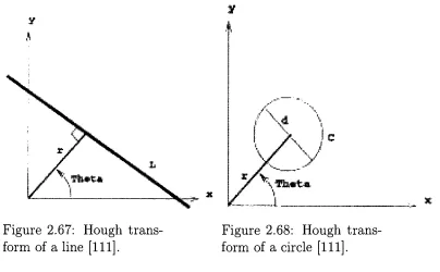
2.67

Hough

transform

of a

line

[111]

Ill

2.68

Hough

transform

of a circle

[111]

Ill

2.69

Hough

transform

of a

line

on pattern 'p'

[111].

112

2.70

Generalized

Hough

transform

of circle on pattern T'

[111].

. .

112

2.71

Fuzzy

set

membership

functions defined

on

Hough

transform

accumulator cells

for

circle

detection from

a pattern of

height

X

and width

Y

[241]

117

2.72

Membership

functions

of

fuzzy

sets

defined

on

Hough

trans

form

accumulator cells.

X

and

Y

denote

the

height

and width

of each character pattern

[240]

118

2.73

Some

of

the

fuzzy

features

extracted

by

Hough

transform

from

eight scanned

Bengali

characters

[240]

119

2.74

Synthesized

fuzzy

set

definitions

using

t-norms

[241]

119

2.75 Chain

code

numbering

schemes:

(a)

Directions for

4-directional

chain code,

(b)

Directions

for 8-direcional

chain code

[175].

. .

120

(21)

2.77

Conventional

(1,

2,3)-Generalized

Chain Code

coding

rings

[288]

122

2.78 Normalized

GCC

8-node

ring

[288]

122

2.79

(a)

The

8-directional Freeman

chain

code;

(b)

The

contour of

a sample

shape,

square;

(c)

Chain

Code

representation of a

square;

(d)

The Chain Code

Histogram

of

the

square

[109].

. .

123

2.80

Example

of

Chain Code

Transform:

(a)

A

45

stroke;

(b)

Same

stroke after

thinning;

(c)

Stroke

labeled

with

chain-codes;

(d)

Transformed

pattern

[44]

125

2.81

Run Length

coding

example

[185]

126

2.82

(a)

Binarized digits

T,'4'

and

'7';

(b)

Digit

covering

with

four

self-affine

transformations;

(c)

Digit

fractal

reconstruction

[9].

128

2.83

'F'

is

covered with six contracted copies of

itself,

each

bar

is

being

covered with

two

contracted copies placed side

by

side

[9].

129

2.84

(a)

Digit

'7'

inside

the

square

box ABCD

and application of

first

affince contraction

resulting in

A'B'C'D';

(b)

Coverage

using

five

contractions;

(c)

Fractal

reconstruction

[9]

129

2.85

Diagram

of

feature

_extraction

by

Fractal Feature for

the

Chi

nese character "Heart"

[247]

130

2.86

Diagram

of

feature

extraction

by

Fractal Feature for

the

_char

acters

T

and 'J'

[247]

131

(22)

LIST

OF

FIGURES

Page

21

2.88 Left:

full

ternary

code.

Right:

4-tuples

with

three

or

four

zeroes removed

[171]

134

2.89

Left:

locations

of

the

two

2-tuples. Right:

Same

two

2-tuples

learning

letter T

and

the

resulting

memory

states

[17].

. . .

135

2.90 System

learning

letter T in

two

different

locations

within

the

image

[17]

136

2.91

Proximity

scores

for

letters lT

and 'A'

[17]

137

2.92

Templates for

characters

*B\ 'G',

'5'

[17]

137

2.93

10 basic

shapes

learned

by

the

system used

in

[17]

138

2.94

(a)

Seven-segment

bar

mask used

for digit

recognition,

(b)

13-segment

bar

mask used

for

alphabetic capital

letters,

(c)

illustration

of

encoding the

character 'S' with shadow projec

tions

shown

in

black

[26]

141

2.95

(a)

16-bar

frame;

(b)A

binary

pattern and

corresponding

shad

ows;

(c)

Normalized

Shadow

Code

[248]

142

2.96 Shadow

codes

for

rotations multiple of90 can

be

obtained

by

simply re-ordering

the

components of

the

code vector

[249].

142

2.97

Bar domains

in

which

the

dashed lines

indicate

(a)

horizon

tal,

(b)

vertical,

(c)

diagonal bars

where pixels

in

each region

project

their

shadows

[215]

. .

143

2.98

32

segment

bar

mask

[229]

144

2.99

Illustration

of

encoding

of

Arabic digit

'8'

(23)

2.100Shadow

mask

for

signature verification.

Left:

An

individual

sampling

square

showing

the

six projection areas

to

be

mea

sured.

Right:

The

signature

is drawn

over a grid of

these

squares.

Bottom: Each

shadowcalculation projects

the

signa

ture

in

each square onto

the

projection areas

[194]

144

2.

lOlFifteen bar

mask representations

[215]

145

2.102Fitting

of

different

templates

to the

pattern

in

question

[93].

.

146

2.103Multiple

templates

for digits

with alternative representations

[93]

147

2.104Ten

templates

fitted

to

an

image

with pattern

in

question

[93].

148

2.105Determination

of an unknown pattern via point

to

point

dis

tance

measurement as performed

by

Elastic

Matching

[220].

.

149

3.1

Differences

in

performance of

RBFN

and

MLPN

as reported

by

different

researchers

if

the

field

of pattern recognition. . . .151

3.2

Model

representation of

MLPN

152

3.3

Model

representation of

RBFN

154

4.1

Examples

of

digits

1 through

6 from

the

data

set utilized. . . .

159

4.2

Examples

of

digits

7,

8,

9

and

0 from

the

data

set utilized. ...

160

4.3

Recognition

accuracy

in

percentages

(vertical-axis)

_achieved

by

MLP

based

on

the

number of

hidden

nodes used

162

4.4

Recognition

rate

in

percentages

(vertical-axis)

achieved

by

(24)

LIST OF FIGURES

Page

23

4.5

Recognition

rate

in

percentages

(vertical-axis)

achieved

by

MLP based

on

the

Alpha/Beta

value used

164

4.6

Percentage

of accurate recognition

(vertical-axis)

achieved

by

RBFN based

on width of radial

basis

centers

165

4.7

Time

required

by

MLPN

and

RBFN

to

fully

train,

based

on

the

size of

the

training

set ...

166

4.8

Performance

of

MLPN

vs

RBFN

on

the

training

sets

ranging

in

size

from

100

to

2500

elements

(horizontal-axis)

withrespect

to

recognition

accuracy in

percentages

167

4.9

MLPN

performance statistics .

168

4.10 RBFN

performance statistics

168

5.1

Classification

of

feature

extraction methods

for

the

various

character representation

forms

[262]

.

171

5.2

Features

from

taxonomy

by Trier,

but

rearrangedand grouped

and methods marked with an asterisk

have been

added

[136].

.

172

5.3

A

dichotomy

'strucuraT

versus

'statistical'

reflects

the

corre

sponding

principles of classification.

The

words

'heuristic' and

'systematic'

refer

to

the way the

features

are selected

[136]

. .

173

5.4

A

taxonomy

proposed

by

the

author

for

the

feature

extraction

methods utilized

in

character recognition

174

5.5

Listing

of

tested

feature

extraction methods with achieved ac

(25)

5.6

Listing

of

tested

feature

extraction methods sorted

by

accuracy.

177

5.7

Listing

of

tested

feature

extraction methods sorted

by

respec

tive

size of

the

feature

vector

178

5.8

Listing

of

tested

feature

extraction methodssorted

by

achieved

accuracy

normalized

for

the

size of

the

feature

vector

180

5.9

Listing

of

tested

feature

extraction methodswith achieved ac

curacy

normalized

for

the

size of

the

feature

vector and

for

random

guessing

182

5.10

Number

of

2D

zones versus

accuracy

183

5.11

Location

of

five

2D

zones versus accuracy.

184

5.12

Confusion

matrix produced

by

the zoning

feature

184

5.13 Number

of

Geometric

moments versus accuracy.

187

5.14

Accuracy

produced

by

different

types

of

Profile

feature

188

5.15 Confusion

matrix produced

by

the

Hough

Transform

feature.

.

189

5.16 Number

of

Fast

Fourier

Transform

coefficients versus accuracy.

190

(26)

Chapter

1

Introduction

The

beginning

of

knowledge

is

the

discovery

of something

we

do

not understand.

Frank Herbert

(1920

-1986)

1.1

Introduction

to

Character Recognition

Since

the

1950's

Optical Character

Recognition,

or

OCR,

has been

an active

field

of research

for

computer scientists worldwide

[262].

The

main reason

is

that

OCR

is

not

only

an

interesting

area of

theoretical

research with rel

evance

to

many

pattern recognition

sub-fields,

but

also a

very

needed and useful real-life application.

Making

computers able

to

read paper

documents

would allow

for

substan

tial

savings

in

terms

of

the

costs

for

data

entry,

mail

processing, tax

form

processing,

census

form

processing

and

many

other similar situations.

Addi

tionally,

this

can

simplify

the

life

of

the

handicapped

by

making

computers able

to

read out

loud

to visually

impaired.

Modern

OCR

systems are able

to

recognize most printed

fonts

and even

some neat

handwritten

text

with acceptable accuracy.

As

a

result, the

cur rent research

in

OCR has

shifted

towards

omnifont machine printed

text,

(27)

1.2

Pattern

Recognition

System

All

complete

OCR

systems consist ofmultiple

processing

steps, namely:

im

age _acquisition,

preprocessing,

feature

extraction, classification,

and

finally,

postprocessing.

In

this

work, we will concentrate on

the

feature

extraction step, since selection of good

features

is

arguable

the

most

important step

towards

achieving

high levels

of

accuracy

by

the

OCR

system.

1.2.1

Data

Collection

Data

collection approaches can

be

as

diverse

as

the

character

data

itself,

from

optical scanners

to

onscreen pointers.

Regardless

of

the

type

of

devise

producing

the

image

of

the

pattern,

data is

usually

collected

in

a

very

raw state.

Typical

sources of

data

include

postal

zip

codes and _addresses, census

form

data,

surveys,

medical _reports, etc.

The handwritten

text

is

typically

comprised of whole words not

isolated

characters and one of

the

first

steps

is

to

break

up

sentences

into

words and words

into individual

symbols.

The

resulting

images

of

individual

symbols are what we need as

input

data

for

the

character recognition system.

1.2.2

Preprocessing

involves cleaning up

the

data

and

trying

to

make

it

as

easy

to

classify

as possible.

The

cleaning

of

data

includes

filling

of gaps and removal ofnoise,

both byproducts

of

image

acquisition process or of

the

later

charac

ter

segmentation algorithm.

Examples

of a

gap

and noise are

demonstrated

in

the

Figure

1.1.

Usually

a

filter

is

used on

the

image

to

close

the

gaps and

to

remove noise

particles,

which are

typically

detected based

on

their

small size with respect

to the

main pattern.

Additional

preprocessing may

be

needed

in

case of color or grayscale

im

ages.

Normally

color

images

are rare and are

easily

converted

to

grayscale.

Grayscale images

need

to

be binarized for

which a

thresholding

algorithm

is

utilized, with

the

finding

of

the

optimal

threshold

value

being

the

most

(28)

1.2.

PATTERN

RECOGNITION

SYSTEM

Page

27

Another

step,

called

normalization, may

be

present

if

we

desire

to

obtain an

image,

which

is

processed

to

counteract

the

effects of

translation,

scaling,

and rotation.

In

each of

those

special situations a particular algorithm can

be

applied:

Translation This

is

the

case

in

which

the

pattern

is

located

off

the

center of

the

image

containing

the

pattern.

To fix

this the

pattern could

be

shifted,

for

example, to the

point where

its

upper-left corner

lines

up

with a particular pixel

in

the

image.

Rotation

This is

the

case

in

which

the

pattern

is

oriented

in

a

way,

which

is

different

from

the

one

in

which

human

reader would

typically

read

it.

This

could range

from

just

a

few degree

of

difference

to

a complete upside-down pattern.

There

is

no

easy

to

apply

solution as

knowing by

how

much

to

rotate

the

pattern requires

first

to

recognize

it,

and

this

of course

is

not possible at

this

step.

Scaling

This

is

the

case

in

which

the

pattern

is

stretched or

truncated

and so

it is

hard

to

recognize

due

to the

difference

in

size.

This is easy

to

fix

by

rescaling

the

pattern

to

some standard size expected of all patterns

being

processed.

(29)

1.2.3

Feature

Extraction

Since

direct

processing

ofscanned characters

images is

computationally

pro

hibitive,

the widely

accepted

technique

of pattern recognition

is

to

extract some

features from

the

original

data

and perform classification on

those

fea

tures.

Extracted

features

must

have

certain properties

in

order

to

achieve

low

error rates

in

character classification.

Features

must provide maximum amountof

information

about

the

original

pattern,

ideally

completely

describ

ing

it.

The

total

number of

features

should

be

minimized

to

reduce

burden

on

the

classification step.

This

means

that

used

features

should

be

indepen

dent

of each other

in

order

to

maximize

entirety

of provided

information

[171]

.

Since

the

same character can

look

very different if it

is

translated,

scaled,

rotated, stretched, or _skewed,

ideally

we are

interested

in

finding features,

which remain constant under

the

above-mentioned morphing.

If

features

with such properties cannot

be

extracted,

an alternative

is

to

use

image

nor malization with respect

to

the

size,

rotation,

and

thickness

of

the

character.

Unfortunately,

this

method

has

a

down

side of

introducing

new errors

into

the

data.

Not

the

least

of

the

good properties of a pattern's

feature is

a

high

tolerance to the

noise and

degradation

in

the

original

image,

as well as

the

complexity

of

the

computation of

the

feature

[262,

171].

An

important

characteristic of a good pattern's

feature

is reconstructability,

which means

that the

feature

contains enough

information

to

reconstruct

the

original pattern.

While

not always _achievable,

reconstructability is

a

desir

able

property

because it

serves as a proof

that the

feature

contains all

the

needed

information

to

recognize

the

pattern

in

question.

For

some

features,

such as

infinite

series coefficients

only

partial reconstruction of

the

original

image is

possible since

only

a small subset of an

infinite

series

is

used as a

feature. The idea is

that

if

such small subset

is

sufficient

to

reconstruct

the

original pattern even

approximately,

the

features

must

have high information

content and so poses

high

discrimination

power

[262].

1.2.4

Classification

Classifier

is

one of

the

most

important

parts of

any

pattern recognition sys

tem.

The job

of

the

classifier

is

to

look

at

the

feature

vector extracted

from

(30)

be-1.2.

PATTERN RECOGNITION

SYSTEM

Page 29

longs.

A large

numberof

different

classifiers

exist,

but

they

all can

be

grouped

under

the

following

headings:

Template

Matching

Each

pattern

is

compared against all other

already

classified patterns and

the

set

to

which

the

closest match

belongs is

selected as

the

probable class of

the

pattern.

Statistical Classifiers In

this

approach a

function

is

designed,

which

has

the

property

of

subdividing

the

feature

space with

hyperplanes

so char acters of

different

types

a separated

into

different

regions.

Artificial Neural Networks

Based

on

the

neural networks

found

in

na

ture,

those

interconnected

tiny

computing

devices

come

together

to

prove

that

sometimes

the

whole

is

greater

than the

sum of

its

parts.

This

is

the

approach often

tried

in

different

fields

of artificial

intel

ligence

and

particularly

in

computer vision and pattern recognition.

Detailed

introduction

to the theoretical

properties of

Artificial

Neural

Networks

could

be

found

in

Chapter

3.

Decision

Trees Determine

type

of

the

pattern

based

on

the

set of

rules;

each

designed

to

further

subdivide patterns until

the

identity

of

the

pattern

becomes

obvious.

1.2.5

Postprocessing

This

is

an optional

step,

which

typically

involves

correction of errors and re

constructionof

the

original

document. Once

each

individual

symbol

has been

recognized, the

symbols are grouped

together to

form

words.

Then

words are compared against a

dictionary

to

see

if

such combinations of characters exist

in

the

language.

A

simple spellchecker could

be

used

to

replace an

unexisting

word with

the

correct one.

Additionally,

the

words

surrounding

the

one

in

question could

be

used

to

improve

the

corrective

ability

of

the

spellchecker.

Such

systems

(31)

Feature

Extraction

Methods

There

is

much pleasure

to

be

gained

from

useless

knowledge.

Bertrand Russell

(1872

-1970)

2.1

Features Utilized

by

a

Human Reader

In

construction of

the

program capable of 'reading5

individual

characters, it

may be

valuable

to

consider

how

the

best-known

system

for

the

purpose a

human

being

operates.

What

features do human

readers utilize

during

char acter recognition process, and could we

teach the

machines

to

use

the

same ones?

Those

are

the

questions

answers, to

which

may

come as

extremely

beneficial

to

construction of a

high

accuracy

pattern recognition system.

It

is

a well-known

fact

that

people

rarely

have

to

recognize

individual

charac

ters

in isolation.

The

typical task

of

reading

consists of

recognizing

symbols,

which make

up

complete words.

As

established

by

many

experiments,

the

meaning

of a

word,

as well as

the

shape of

the

wordcontribute

to the

correct

recognition of

individual

characters.

This is something

not

typically

pro grammed

into

the

character recognition

software,

at

least

not prior

to

a

few

years ago

[272].

In

research

into reading,

as

in

most of

psychology,

observing

the type

of

errors made under

hard

circumstances

is

a

very

fruitful

type

of

investigation.

(32)

2.1.

FEATURES

UTILIZED

BY

A HUMAN READER

Page

31

subjects

during

the task

of character recognition.

He

presented character symbols

to the

subjects at a

distance

or

for

a

very

short

duration

of

time,

and examined

the

confusions made

between different

letters. Bouma

grouped

the

characters of

the

English

alphabet

into

sets

based

on

the

errors made

by

the

subjects

in

his

experiments.

The Bouma's

classification oi

psychologically

close

letters

is

presented

in Figure 2.1.

Outer

contour

Bouma

shape

Code

Letters

Short

inner

parts and rectangular envelope

1

a s z x

round envelope

2

e o c

oblique outer parts

3

r v w

vertical outer parts

4

n m u

Tall

ascending

extensions

5

dhkb

slenderness

6

t

i

1 f

Projecting

descender

7

g

j

p q y

Figure

2.1: Bouma's

classification of

letters

[272].

The

classification consists of

three

large

sets,

namely

Short,

Tall

and

Projecting

characters,

which are

further

subdivided

into

as

many

as

four

subgroups with

up to

five

characters

in

each.

The

actual

features believed

to

be

used

by

human

readers

vary

by

a re searcher.

Hubel

and

Wiesel

believe

the

features

are generated

early in

the

visual cortex.

The

complex cells

they

found detect

the

presence of

bars

and edges and provide a representation of

lines.

McGraw

et al. conducted exper

iments

with machine printed characters and

found

that

high-level

structural

descriptors

of

letters

are

very

likely

utilized.

For

example,

a

letter

'b' could

be described

as a

loop

with a stroke attached at

the

lower

right.

Intuitively,

this

latter

representation seems

very

close

to

a

human

heart,

but

we can not

dismiss

the

value of unconscious processes

[272].

Later

in

the

chapter we will see

that

both

types

of

features

are

indeed

put

(33)

2.2

Image

Partitioning

Approaches

2.2.1

Zoning,

a.k.a.

Sub-

window

Pixel

Count

The

method of

zoning

was

introduced in 1972

by

Hussain,

[107].

It is

one of

the

easiest

feature

extraction methods

in

terms

of

implementation.

The

feature

produced

is

an

array

of

integers representing

the

number of

turned-on pixels

in

the

sub-windows of an original

image.

Refer

to

figure

2.2

for

a visual representation of

the

above

idea.

Figure

2.2:

Upper-left:

character

A;

Upper-Right:

Zoning

_grid

imposed;

Lower-Left:

binary

zoning

feature;

Lower-Right:

_{sub-window pixel counts}

In

more

formal

terms

the

idea is

to

_sub-divide

the

bilevel

image into K

non-overlapping

regions or zones

Ri,

i

=

1...K,

each of size

h

x v.

In

this

case

the

feature

f

is

the

number of

foreground

_pixels

in

i^.

This

(34)

2.2.

IMAGE PARTITIONING APPROACHES

Page

33

The

number of

sub-windows,

K,

used

during

feature

extraction,

can

vary

from

as

little

as

one, giving

us

the

area of

the

binary image,

to the total

num

ber

of pixels

in

the

image,

h

v,

resulting in image itself.

Smaller

sub-window

size results

in

better

discriminatory

performance,

since

in

large

sub-windows

important

pattern

information

gets smashed.

Typically,

a window size of

4x4

or

8

x

8

is

used.

The

resulting

feature

vector remains

relatively small,

even as a size of

the

input image increases. For

example,

even

in

a small

30

x

30

pixel

image using 5x5

sub-_{windows we end}

up

with a

36-dimensional

vector.

In

the

original paper

Hussain

et al.

[107],

summarized

the

desirable

proper

ties

of

their

proposed

feature

extraction algorithm as

follows:

The feature

vector

is

obtained

from

the

pattern matrix

by

a repetitive

procedure

involving

only

the

simple

logical

operation of

counting

the

number of

black

points

in

a well-defined region.

The

feature

vector's

dimensionality

is significantly

lower

than that

of

many

other schemes and

the

features

themselves

assume

only

a rela

tively

small number of values.

Discontinuities

in

the

character

matrix,

including

salt and pepper

noise,

can

be

tolerated

[107].

An

additional reduction

in

the

complexity

of an extracted

feature

can

be

achieved

by

replacing

pixel counts

for

each sub-window with a

binary flag

signifying

state of

the

pattern

in

this

region.

See bottom-left

of

figure

2.2

for

an example of so called

binary-zoning

feature.

Unfortunately

this

strategy

significantly

reduces a

discriminatory

ability

of

the

zoning

feature.

In

addition

to

being

applicable

to

binary

images,

zoning

can

be

used on

gray

scale

images

as well.

In

order

to

extract

the

feature

vector,

an average

gray

level is

computed as can

be

seen

in

figure

2.3.

Unfortunately,

the

re

sulting

feature

is

not

illumination invariant

[262].

Zoning

method

is

a universal

feature

extractor,

capable of

operating

on

bi

nary, gray scale, contour,

and even skeleton character representations.

But,

it

does have

some obvious

problems,

such as

its

lack

of

tolerance

for

either

rotation, shifting

or scaling.

While

invariance is

a

desirable

property

of a good

feature,

through

some clever

preprocessing

we can almost

completely

(35)

4

mmWT. mm

1

w

%

|

:

'

i

=:-(a)

0>)

Figure

2.3:

Zoning

on a

gray

level

image,

(a)

A

4

x

4

grid on a

gray

scale

character,

(b)

The

resulting

average

gray

levels for

each zone

[262].

Zoning

Pseudonyms

It

is

a well-known

fact,

that

sometimes

in

the

process of scientific

discov

ery

different

researches stumble upon

the

same

idea

independently

of one another.

Nothing

is

truer

about

feature

extraction

methods,

in

particular

Zoning. While

it

is

namely

_{normalization process}

in

_which

the

sum of

the

pixels

in

each subwindow

is

being

divided

by

the

total

number of pixels

in

that

zone,

resulting in

the

black

pixel

density

for

that

region.

The

same

feature

without modifications

is

called

Averaging

Algorithm

in the

_paper

by

Toroketal.

[261].

Finally

Hanmandlu

et al.

[92]

refers

to

it

as

Box

Approach.

Such

multitude ofnames makes comparisonofworks

by

different

_researchers

more complicated and

hopefully

this

thesis

will

be

a

step towards

universal

naming

convention

for

different features

used

in

character recognition.

2.2.2

Fuzzy

Zoning

The

method of

Fuzzy

Zoning (FZ)

developed

by

the

_author

is

_aimed

(36)

2.2.

IMAGE PARTITIONING

APPROACHES

Page

35

position and

size,

which cause problems

for

the

classical

zoning

approach

BBMP'

! *.*l*****4l

Figure

2.4:

Fuzzy

contribution of pixels

located

in

a corner or

in

a middle of

a pattern.

The

main problem with

the zoning

method

is its

reliance on

rigid

zone

borders.

Each

pixel either contributes

to

a particular zone or

does

not,

de

pending

on

its location. This has

particularly

negative effect

in

case of

near-border

pixels as even

the

smallest shift

in

the

pattern results

in

a

different

feature

vector.

Cao

at el. attempted

to

counteract

this

problem

by

creating

something

called

Fuzzy

Borders

(FB).

The

main

distinction

of

FB lays

in

the

fact

that

points of

the

pattern

located

near zone

borders

are given

fuzzy

membership

values

in up

to

four

zones at

the

same

time.

Fuzzy

membership

values are normalized

by

always

adding

up to

one

for

all zones

[31].

Taking

the

idea

behind

FB

and

expanding

on

it

we came

up

with

the

concept of

FZ.

Unlike

in

a case of

FB

in

which

only

border-pixels

have

fuzzy

proper

ties

and

only in up

to

four different

zones,

our method gives all pixels

fuzzy

(37)

image

depends

on

its

relative

location

within

the

zone as well as within

the

global pattern.

Figure 2.4

demonstrates

this

idea.

Pixel PI located

in

zone

CA

contributes

heavily

to

that

zone since

it is

located

almost

in

a middle of

it,

but

it

also contributes,

but

to

a much

lesser

extent,

to

zones

CB,

BB

and

BA. Pixel

P2

located

in

zone

BC

also contributes

heavily

to

its

home

zone,

but

it

also_contributes,

to

zones

AD, AC, AB,

BB,

CB, CC,

CD

and

BD.

The

actual contribution of each pixel

to

each zone

depends

on

the

distance

between

the

pixel and

the

zone and

is automatically

calculated

by

performing

multiplication operation

between

the

original pattern and

the

special fuzzy-mask

developed

by

us.

The fuzzy-mask

is

a

group

of concentric squares whose weighted value

diminishes

linearly

as

the

distance from

the

center of

the

mask

increases.

Figure 2.5 is

a sample

fuzzy-mask

with

linear decrease

in

10

percent

for

each concentric square.

By

moving

the

fuzzy-mask

across

the

entire original

pattern,

we were able

to

obtain

FZ

feature

vector

consisting

of

25

individual

elements each

representing

a unique zone and

the

fuzzy

contribution of

the

zone's neighbors.

Figure

2.5:

Fuzzy

mask with

linear decrease

in

10

per

(38)

2.2.

IMAGE PARTITIONING APPROACHES

Page

37

*4M

7

/

r

l I \

Figure

2.6:

Discriminative

ability

of

local information

[192].

2.2.3

Zoning

-

image

was sub

divided

into

zones and

for

each zone an area of

the

character pattern

falling

in

that

zone was computed.

The

concept of

zoning

can

be

abstracted

into

the

so-called

meta-feature, by

saying

that

it simply involves

breaking

the

original

image

into

a number of subzones.

The

resulting

subzones can

be

processed

with

any

feature

extraction method

described

in

this thesis.

The

resulting

feature

vectors can

be

concatenated

into

one comprehensive

feature

vector

describing

the

overall pattern.

The

main advantage of

the

zoning

meta-method

is

that the

properties of

individual

subparts of

the

image

are not

mixed,

but

extracted separately.

This

allows

for local information

to

play

a more significant role

in

pattern classification.

It is

a well-known

fact

that

local information

is

often all you need

to

distinguish

patterns

belonging

to

a particular subset of all possible patterns.

Figure 2.6 demonstrates how digits

'3' and '5' can

be

ruled out

if

lo

cal

information

in just

one subzone

is

more

typical

of a

digit '7's

pattern

[192]

.

(39)

de-A

B

C

llr r.

D

1

E

1

F

P2

G

H

1

Figure 2.7:

Zoning

method with

fuzzy

borders. Pixel

P\

has

a

fuzzy

mem

bership

value of .25

in

each of

the

four

zones

A,

B, D,

and

E.

P2

has

a .75

membership

value

in

zone

E

and .25

in

zone

F

[262].

gree of variation

into

the

feature

subvectors.

The

subpatterns

may

show

up

differently

in

subwindows

due

to

even small shapevariations

in

the

wholepat

tern,

resulting in

radical

differences

in

the

values computed

for

subvectors, which

in

turn

makes

the

concatenated

final feature

vector

less

continuous pattern

descriptor

[136].

Cao

at el. attempted

to

counteract

this

problem

by

creating something

they

called

fuzzy

borders. The

main

distinction

of

fuzzy

borders

is in

the

fact

that

points of

the

pattern

located

near zone

borders

are

given

fuzzy

membership

values

in

up to

four

zones at

the

same

time.

Fuzzy

membership

values are normalized

by

always

adding

up to

one

for

all zones

[31].

Figure

2.7

demonstrates

zoning

with

fuzzy

borders.

Since

the

zoning

method as presented

here

is

just

a

way

to

break

up

the

original

image,

we are still

faced

with a choice of

feature

extraction method

to

be

used with our subdivision approach.

Different

researchers

have

tried

out

different feature

extraction methods with

varying

degrees

of success.

Examples

of some of

the

features

utilized are

described below.

In

general,

(40)

2.2.

IMAGE

PARTITIONING APPROACHES

Page

39

J

^^

3

(

/

<

N,

\.

/

V

(a)

orientation count

0 45 90 135

9

1

2

4

(c)

Figure

2.8:

Zoning

combined with contour

line

segment counts,

(a)

character subdivided

into 16 equally

sized

zones;

(b)

contour

lines

in

the

upper-right zone

only;

(c)

count of contour

lines for

this

zone.

[262].

Kimura

and

Shridhar

worked with contour curves as

the

pattern representa

tion technique.

After

applying zoning

they

grouped

the

contour

line

segments

based

on orientation

into four

subgroups,

namely:

horizontal,

vertical,

diag

onal (45 and

135)

orientations.

The

number of contour segments

belonging

to

each

group

was used as

the

extracted

feature for

each zone.

Figure 2.8

demonstrates

this

approach

[125].

Another

researcher,

Takahashi,

also used

orientation

histograms,

but

in

addition

he

also

found high

curvature points

along

the

contour.

For

each such

point,

Takahashi

computed contour

tan

gent,

curvature

value,

and position within

the

zone

[262].

Singh

and

Hewitt

[231]

used a modified

Hough

transform

(see

Section

2.6.3

for

details)

in

combination with nine

3x3

windows

in

their

work on cursive

digit

and character recognition.

(41)

000 00001 000000 000000000000000 0 OODOOOOIQOOQOO00000000000 00000

00000001000000 00600000000 00000

OOOOOO I I ! 1)110 l I IHH!IHHMHJ flit

00000100000000 0000000000000800

OOOOI00OQOOOOO0000009000000011 000 IfOAAOAOOOBOA0O0O0OO6AAOO1 8 OOO1OO0O0OO0O00O0O0OOO0O0OOI00

ODD10000000 UO0O0BU 00 0O0O0OO100

001O0O0O0OO0O8OOO0OO0O000O1000 OOIOOOOOOOOODOOOOOOOOOOOQI1000 0100000 0000000 0000 0000000 16000 I I000O0OO0O00009OQ00OO0OO10000 100000000000000000000000110000

lOOOAOOAOAOOAAOAOOOOOOOOIOOOOO

I1 1 00000000 0000000 OOOOOO I 00000 OH 1000000000OO00 000000 0100 0000

0001 I000000000 00 00 ODOOO I OOOOOO

n n minii1 1 nnnnnnnnnnnnnninnnnnn 00000000011 I 100O0000OO01OO0000 000000000000011100000001000000 OOOOOOOOOOOOOOOOI 1I 1I1 II t 11000 OOOOOOOOOOOOOOOOOOOOOOIOOOOIIO

0OO00O0OOOO0OOOOD000010OO0000I

OOOOOOOO 000 0000000000100000000 000000000000000000001100000000 0000000 0000001000000 1000000000

OOOOAOOOO0OOOBAAOOAO1OAOOAAA0A

OOOOOOOOOOOOOOOOOOOIOOOOOOOOOO U IMRHHI t) UO UllUIHUIOU1MMUOOOOOOOUU OOOOOOOOOOOOOOOOOOOIOOOOOOOOOO OOOOOOOOOOOOOOOOOOOIOOOOOOOOOO (a) _^_ " .

12 3 4

(c)

Figure 2.9:

(a)

Normalized

digit

4.

(b)

Digit 4

partitioned

into 6x4 boxes.

(c)

pattern of

digit

4

plotted

using

extracted

features

[92].

For

example

in

[92]

bottom

left

corner of

the

original

image is

used

for

such purpose.

The

vector

distance for fcth

pixel

in

6th box

at

location

(i,j)

is

calculated as,

d\

= (i2

+ j2)'5.

By dividing

the

s