MoL 2011 04: Variable Binding in Biologically Plausible Neural Networks

VARIABLE BINDING IN BIOLOGICALLY

PLAUSIBLE NEURAL NETWORKS

MSc Thesis

(

Afstudeerscriptie

)

written by

Douwe Kiela

(born June 7th, 1986 in Amsterdam, the Netherlands)

under the supervision of Prof. Dr. Michiel van LambalgenandDavid Neville, M.Sc., and submitted to the Board of Examiners in partial

fulfillment of the requirements for the degree of

MSc in Logic

at theUniversiteit van Amsterdam.

Date of the public defense: Members of the Thesis Committee:

August 30, 2011 Prof. Dr. Michiel van Lambalgen Prof. Dr. Frank Veltman

Contents

1 Introduction 3

1.1 Acknowledgments . . . 4

2 Background 5 3 The Binding Problem 9 3.1 Solutions to the Binding Problem . . . 12

4 Connectionism and Computational Neuroscience 16 4.1 Connectionism . . . 16

4.2 Computational Neuroscience . . . 18

4.3 Biological Plausibility and Logic . . . 22

5 Methodology 24 5.1 Spike-Time Correlation . . . 24

5.2 The NeoCortical Simulator . . . 25

5.3 Parameters . . . 26

6 Models and Results 28 6.1 Model I: Testing Correlation . . . 28

6.2 Model II: The Impact of Inhibition . . . 29

6.3 Model IIIa: Conductance . . . 31

6.4 Model IIIb: Firing Rate . . . 32

6.5 Model IV: Lover and Lovee . . . 33

6.6 Model V: Little Big Star . . . 34

6.7 Model VI: Single Binary Predicate Variable Binding . . . 35

6.8 Model VII: Multiple Predicate Variable Binding . . . 36

7 Discussion 39 7.1 Conception of Logic . . . 39

7.2 Logic Programs and Neural Networks . . . 41

7.3 Incorporating Rules . . . 43

7.4 Determining the Threshold . . . 45

8 Conclusion & Outlook 47

A Detailed Graphs and Plots 49

B NCS, Brainlab and Code from the Experiments 57

B.1 Installing NCS and Brainlab . . . 57

B.2 Understanding NCS and Brainlab . . . 59

B.2.1 Setting the parameters . . . 59

B.2.2 Constructing the network . . . 60

B.2.3 Running the simulation . . . 61

B.2.4 Analyzing the results . . . 61

Chapter 1

Introduction

One of the most essential aspects of logic is the ability to bind variables. Without that ability, we cannot represent generic rules in a logical form. In the past decades there has been a lot of interest in implementing logic on neural networks, but this was largely restricted to propositional logic. There have been attempts to implement more sophisticated logics on neural networks, with mixed success. So far, there have been no results that conclusively (and non-theoretically) show that first-order logic can successfully be implemented on neural networks. The most important step towards doing just that, or at least doing so for a fragment, is implementing variable binding on neural networks.

In the study of logic and neural networks, the connectionist paradigm has been of pivotal importance all across the domains of cognitive science. How-ever, one might consider traditional connectionism slightly outdated or oversim-plified compared to our current knowledge of the workings of neurons and the brain. Since the advent of the original artificial neural networks, the discipline of computational neuroscience has made significant progress. The fine-grained dynamics in such models may provide new insight into the relative standstill that the study of logic (using variables) and neural networks has suffered from in recent years. This interrelation has, so far, been largely unexplored for these biologically more plausible models.

Chapter 4 makes explicit the distinction between connectionism and computa-tional neuroscience, in order to draw attention to biologically plausible neurons. Chapter 5 briefly describes the methodology. The correlation between spike times as a measure for binding is described and the software chosen to perform the simulations is introduced, as well as the software used to analyze the results. Since biologically plausible networks are necessarily highly parameterized, the chosen parameters are discussed as well. The next chapter will turn to the actual experiments used to show that such networks are indeed capable of performing variable binding. Several criteria have been set in the preceding chapters, which will be addressed in the models. Chapter 7 will briefly discuss these results and shed light on some of the remaining issues. Moreover, it discusses the concep-tion of logic that is at the base of what the thesis proposes; and discusses some important aspects of extending the research presented. The closing chapter will look back on what has been covered in the thesis and provides a brief roadmap towards achieving the final goal of implementing first-order logic in full.

1.1

Acknowledgments

Chapter 2

Background

From a logical standpoint, the development of artificial neural networks has al-ways been heavily intertwined with propositional logic. The very first artificial networks introduced by McCulloch and Pitts in their seminal 1943 paper [58] equate individual nodes with propositional formulae. The discovery by Min-sky and Papert that McCulloch-Pitts networks could not implement exclusive disjunction [61] resulted in a decline in artificial neural networks research, but the subsequent development of the backpropagation algorithm [101][73] led to a renewed interest from the early 80’s onwards.

The line of thought that emerged from this renewed interest was at first predominantly an artificial intelligence affair, but soon awakened the interest in philosophers. TheStanford Encyclopedia of Philosophydescribes connectionism– as the line of thought is known–as “a movement in cognitive science which hopes to explain human intellectual abilities using artificial neural networks”, which “promises to provide an alternative to the classical theory of the mind: the widely held view that the mind is something akin to a digital computer process-ing a symbolic language” [30]. For our current purposes it is not necessary to go into the full details of the so-called connectionist-symbolic debate (but see e.g. [72]). However, it is important to note that this distinction and the alleged incommensurability [18] of the two paradigms has inspired prolific research into the general topic of the thesis at hand, namely the implementation of logic on neural networks.

energy distribution of networks, with Pinkas arguing that the global minimum in the energy function of symmetric networks corresponds to finding a model for a propositional formula [67] (another example is [11]). G¨ardenfors & Balke-nius showed that neural networks perform non-monotonic reasoning [8]. Even recently, new models of neural networks have been developed that use logic as a base [76].

The popularity of the logic programming paradigm [54] in the study of arti-ficial intelligence opened a way to exploit the ability of networks to learn facts (i.e., the declarative side of logic programs) and at a later stage to process the network and examine the inputs and outputs (i.e., the procedural side) in a logically rigid way [37]. What is more, logic programs are ideally suited to incorporate non-monotonic reasoning, through for example negation as failure or completion algorithms [29]. The study of propositional logic programs and artificial neural networks yielded impressive results. For example, H¨olldobler et al. were able to develop a connectionist system for computing the least model of propositional logic programs, provided such a model exists [38]. However, all studies mentioned above have in common that they are focused on propositional logic. The lack of research into more expressive logics famously led McCarthy very early on to pose overcoming “propositional fixation” as one of the major challenges facing connectionism [57].

Answering McCarthy’s challenge, however, has proven extremely difficult. The vision presented by Smolensky [83], where connectionist systems fully in-corporate the power of (first order) symbolic logic, is still far from complete. Numerous attempts have been made, with mixed results. Unary relations were modeled in [9] and predicates with higher arity and inference rules were mod-eled in [79] and [47]. Although these attempts were successful within a limited scope, nobody has come up with a theory as of yet that conclusively settles the issue once and for all. Quite obviously, classical logic would be the most desirable, but the apparent inability to come up with any conclusive results has caused some researches to move away from classical first-order logic and towards things like “connectionist modal logic” [20]. However, positive results have been obtained for first-order fragments of classical logic: H¨olldobler et al. were able to prove that the least model of first-order logic programs can be approximated arbitrarily well by multi-layer recursive networks with a feed-forward core [39]. First-order logic programs are an especially suitable candidate, not only because of the aforementioned properties of logic programs in general, but also because they do not require an external (and potentially infinite) domain, like classical logic would. Instead of a Tarskian semantics based on objects in the domain, first-order logic programs apply unification to satisfy clauses, using substitution of identical (or equal) terms [4].

(i.e., atomic formulae) and complex formulae that consist of combinations of atomic formulae and logical connectives.

The issue of representation coincides with another heated philosophical de-bate, namely, whether “meanings” are represented at all. The sentence John loves Mary may be encoded using a distributed representation that does not contain any explicit representation of the constituents John, loves, and Mary [84]. Even though these constituent representations can be retrieved from the network, the network itself does not need to retrieve them in order to process the entire sentence correctly [17]. These distributed representations are the oppo-site of localist representations, where every constituent is assigned a single node that represents it (like McCulloch-Pitts neurons, for example). In the past these localist representations have been criticized on the basis of the Grandmother-cell analogy [18]: if my grandmother is represented by one single neuron, what happens when that neuron is damaged? Do I forget my grandmother? Psy-chological and neurological evidence suggests that this is not the case and that seeing your grandmother triggers a pattern of neural activation distributed all over your brain.

Distributed representations are often portrayed as incompatible with the symbolic paradigm, which is said to be inherently localist. In this sense, dis-tributed representations have several advantages: they allow for the combination of not-necessarily-propositional content, such as olfactory or kinesthetic data, with propositional content and they are robust in the sense that minor damage does not destroy the representation–which allows distributed representations to degrade gracefully. The idea is based on a theory proposed by Donald Hebb, which proposes that neurons that are distributed all over the brain form as-semblies (i.e., neurons become associated with each other) by firing together [36]. Thus, your grandmother is represented by a Hebbian assembly, which was formed through Hebbian learning–under the motto “fire together, wire to-gether”.

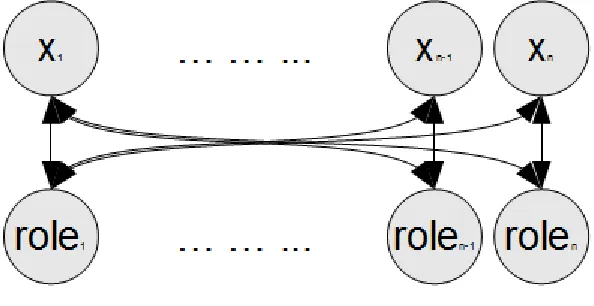
loss of generality, interpreted as a neural assembly–a distributed representation, in other words. Thus, when we want to represent terms, predicates and for-mulae in a neural network, our primary decision is what we will choose as our atomic data, which will be given a localist representation. In our case, of course, the most primitive constituent is a term; specifically, constants and variables. However, there is more to it than that. Consider the following predicate:

P(x1, x2, ..., xn)

Where constants and variables are the fillers for the predicate’s arguments, we also have to keep track of which filler is associated with which argument. In other words, we have to know the role of the constants and variables in the predicate. Taking these considerations into account, the most basic spatial representation of an n-place predicate would be something along the following lines1_:

Figure 2.1: Representing a Predicate in a Neural Network

All available constants and variables are connected to all the available roles of the predicate, because all constants and variables can bind to all these available roles. However, this leads to a problem: how can we represent these bindings in such a way that we can distinguish multiple encodings and find the correct bindings? That question is the topic of the following chapter.

1_{As we shall see, an important aspect of neural network models that is lacking in this}

Chapter 3

The Binding Problem

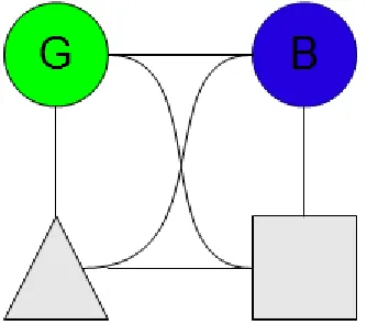
A single predicate is arguably one of the simplest forms of a combinatorial structure we can possibly encode in a neural network. However, combinatorial structures have been the root of a substantial challenge to connectionism and neuroscience, known as the binding problem. The binding problem occurs in many different shapes and guises. As a result, the term is applied to a wide variety of not necessarily related instances where “binding” can occur and cause problems. In its simplest form, the binding problem concerns the way in which neural instantiations of parts can be bound together in a manner that preserves the structure of the whole that is made up out of the parts. To give an easy and well-known example which was first given by Rosenblatt [71], consider a simple neural network that is given the task to encode and retrieve two colored shapes: a green triangle and a blue square.

The neural instantiations of the parts, the constituents of the color-shape com-binations, are green, blue, triangle and square, respectively. The problem arises when we want to distinguish between the two shapes: the color green has to be bound to the shape triangle, whereas the color blue has to be bound to the shape square. We are unable to represent both structures in the same network and be able to tell them apart, because there is no way to determine which color belongs to which shape.

For example, consider the two color-shape combinations encoded in a simple Hopfield network with a binary activation function, with the nodes in Figure 3.1 as the nodes in the network. In order to represent the green triangle, the nodes Green and Triangle have to be activated. For the blue square, we need Blue and Square to be active. When both are active at the same time, the tri-angle and square could be either green or blue: there is no way to tell them apart.

A problem by the same name has been heavily debated in philosophical dis-cussions of the so-called unity of consciousness. The problem roughly comes down to the issue of how all our perceptual experiences can be combined–that is, bound together–into one big picture, a “Cartesian theatre”, which we call conscious experience. A similar problem is found in binding data from different modalities, i.e. auditive and visual perception. Although an important issue in its own right, this type of binding problem is not what is at stake when we are looking into encoding predicates on neural networks. Hence, in order to be as clear as possible, it is important to clearly demarcate the particular instance(s) of the binding problem that we are faced with.

In the context of the neural instantiation of linguistic structures, i.e. the combinatorial and rule-based structure of language, Jackendoff [42] has pre-sented “four challenges for cognitive science”, all pertaining to a particular type of binding problem. As Jackendoff himself has acknowledged, although his book is about linguistic structures, the same problems apply to any combinatorial structure we wish to give a neural instantiation. The four challenges are (see also [55]):

1. The massiveness of the binding problem

2. The problem of multiple instances

3. The problem of variables

4. The relation between binding in working memory and binding in long-term memory

we distinguish that sentence fromMary loves John? Another favorite example isThe little star is beside the big star, which involves a much higher number of bindings than the typical example of the visual binding problem sketched above [31]. This sentence also confronts us with Jackendoff’s second challenge, namely, the word “star” is used twice, but binds to different attributes (little and big). The problem is, when we have multiple instances of the word star, how do we ensure that the right binding is used at the right moment, and how do we avoid erroneous bindings such aslittle big star? Even if we are able to solve these two problems, we have only solved the binding problem for the knowledge of specific facts. But how about systematic facts, such as the fact that gives(x,y,z) entails owns(y,z)? We could encode it for the case ofJohn gives Mary a book, but then what happens when Bob gives Mary a book? Obviously, we would want our neural instantiation of such a rule to be systematic enough to be able to deal with any case in which the rule applies. In other words, the rule has to be generically encoded, such that we can instantiate the variables at a later stage. It is easy to see that the amount of binding necessary for such a case is much larger than in the first two cases, because objects or attributes need to bind to variables, which in turn need to bind to their respective arguments in give and own. This, the third challenge, is known as the variable binding problem, which is an important problem since rule-based relationships play such an important role in human cognition. And then there is also the question of where and how this binding takes place in the brain. Working memory is typically assumed to consist of activity in neurons that encode the information that is currently active in the working memory [26]. That is, a piece of information only stays in working memory for so long as the activity encoding that information is sustained [27]. On the other hand, long term potentiation, which is associated with long-term memory, results from synaptic modification in the connections between neurons. Jackendoff’s last challenge is about understanding how the interface between these two types of memory occurs, specifically when it comes to the type of binding that happens.

All four challenges are important for incorporating order logic, or first-order fragments, on neural networks, but the central issue is the variable binding problem. In order to solve the variable binding problem, we first need a good solution for the first two problems. Jackendoff’s last challenge is a little different. It does not directly relate to our current topic of interest, but the way you choose to implement variable binding for predicates is directly related to how you want to answer that question. Any theory that claims to “solve the binding problem” needs to answer at least the first two challenges. The answer to the fourth challenge is a consequence of the choices made for the implementation, so biological plausibility in that sense would give the theory as a whole more credibility.

strict constraints variable binding imposes on rule-matching may be necessary for modeling human language acquisition (see also [68]). Browne and Sun char-acterize variable binding as a form of complex pattern matching, with three main forms, from simplest to most complex:

1. Atomic symbol matching. When we teach green(triangle) and then ask the network whether the triangle is green, it should reply yes.

2. Standard pattern matching. Teaching green(triangle) and then asking the networkwhat is green, i.e., green(X), it should reply X=triangle

3. Unification. When both pattern and datum can contain variables. When we teach dog(X) and ask dog(Y), then it should give us Y=X, even though both are variables.

Taking that characterization of variable binding as a roadmap for coming up with a possible solution, we should start off with the simplest form, atomic symbol matching. This corresponds to the simplest binding problem. From there on out, we can try adding more and more complexity.

3.1

Solutions to the Binding Problem

Over the years, many different solutions to the variable binding problem have been proposed, all in varying detail and coming from very different disciplines in the spectrum of cognitive science. Broadly speaking, two main strands can be discerned in all these different theories: the temporal and the spatial solution.

At first glance, the spatial solution seems a very natural answer to solving the binding problem: if we have to encode a blue square and a green triangle, why don’t we simply have one neuron for a blue square and one for a green triangle? However, this quickly leads to the neural equivalent of combinatorial explosion. Psychological studies suggest common knowledge in humans amounts to as much as 108 _{items [51]. Given that we only have about 10}12 _{neurons in}

the brain by most estimates and that most of these neurons are likely to be involved in other processes than knowledge processing, there is no way we could encode combinatorial structures like this–let alone when we want to encode more properties, such as abig equilateral flashing dotted soft furry green triangle, just to name something.

type of variable binding–unification [97], as have Kohonen maps [44][98]. How-ever, in general these spatial approaches have been faced with much criticism. It has been noted that the vectors are not of a fixed dimension, making them very impractical computationally [31]. Apart from the combinatorial explosion that renders the spatial models neither biologically plausible nor computation-ally feasible, it has also been noted that they tend to operate in a serial fashion, whereas cognition is known to be parallel [79].

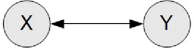
Due to the spatial and quantitative constraints on the human brain and re-search in the 1980s that suggested synchronous firing–“gamma oscillations”–in the cat’s visual cortex, temporal binding was presented by von der Malsburg as a viable alternative to solving the binding problem [95]. Specifically, the timing of spikes in neural networks, or the local field potential of neural assemblies, could be used to bind the combinatorial aspects of a structure. For example, if green and triangle fire together, they are bound together. This idea is also strongly related to Hebbian learning and Hebbian assemblies [36]. Traditional rate models, such as the Hopfield network with binary activation that we dis-cussed earlier, do not take the actual firing times of neurons into account. If we look at the firing times of neurons encoding green, blue, triangle and square, we can see that the respective neurons for green triangle and blue square fire in synchrony, but that they have identical firing rates.

Figure 3.2: Different Spike Times with Identical Firing Rate

The temporal model has been suggested pretty early on as a particularly good way to solve the variable binding problem [25][96]. The approach has met with quite some success in a large range of problems of brain function [34] [82]. But it is important to note that there are also constraints on the temporal model, mostly derived from psychological experiments. A system that applies a temporal solution to the binding problem has to be able to perform binding at a reasonable time interval, one that is comparable to humans.

binding. These representations were subsequently used to form rules, where the synchronous oscillations propagate through interconnected representations.

Their neuron-like elements are idealized oscillators of four different types:

1. τ-and nodes: produce an oscillatory pulse with same period and pulse width as its input

2. ρ-btu nodes: produce a periodic spike train in phase with the input spike train1

3. τ-or nodes: become active when it receives one or more spike signals within one oscillatory period

4. Multiphase τ-or nodes: become active when it receives more than one spike trains, in different phases, during the same oscillatory period

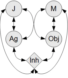
Using these elements, Shastri & Ajjanagadde are able to encode an n-ary predicate P using two τ-and nodes and n ρ-btu nodes. By connecting these nodes in specific ways, facts and rules can be encoded that amount to a signicant fragment of Horn-clause logic. Using these nodes, synchrony between John and Lover and Mary and Lovee encodes which role (lover, lovee) in the predicate is taken by which filler (john, mary). In a similar fashion to Abeles’ synchronous firing chains [2], the synchronous pattern propagates through the chain, allowing an antecedent predicate to enable the consequent predicate. It is beyond the scope of the thesis at hand to go into full detail, so suffice it to say that the network is constructed such that the nodes form a pathway towards a certain inference.

Shastri & Ajjanagadde’s results were enthousiastically received and still form the basis for many explorations of the binding problem that make use of tem-poral solutions. The model has also been extended to model larger fragments of Horn clauses and a larger set of inferences, such as in [63] and [64]. Oscil-lators have also been used in completely unrelated ways but much to the same purpose, such as in [89] and in [91].

In addition to what we may call the strictly-spatial and strictly-temporal ap-proaches, many hybrid approaches have emerged which do not clearly subscribe to either of these paradigms. Fortunately a number of excellent overviews and surveys exist, most notably [5], which provide an adequate excuse not to discuss these in detail. Approaches that fall in this category are theories that do not acknowledge the necessity of representing combinatorial structures at all (see [92] ch. 4). Theoretical work that exemplifies this approach and that deserves distinct mention is recent work by H¨olldobler et al. [7] which tentatively and pre-liminarily extends their so-called Core model to first-order logic. Furthermore, hybrid approaches such as blackboard models [92], signature-based processing (e.g. [14]) and combinations of these approaches [10] have been proposed in recent years.

1_{It is unclear what the lettersbtu are supposed to stand for. Suffice it to say that these}

Chapter 4

Connectionism and

Computational

Neuroscience

As was already briefly discussed in the previous chapter, spatial solutions to the binding problem were inadequately equipped to fit within the known constraints of the human brain. It is important to note that this fact does not at all disqual-ify any such theory, as indeed there are many more interesting applications of connectionism outside the particular domain of understanding human cognition. For example, as Bader & Hitzler make clear in their survey of neural-symbolic integration, integrating connectionist and symbolic knowledge representation may also be motivated from a more technical perspective, for example by trying to find optimal ways to combine the advantages of both approaches [5]. The same constraints of course do not apply in this domain, which is particularly relevant for computer science-related applications of knowledge representation. For the thesis at hand, however, we are predominantly concerned with biologi-cal plausibility, because a more biologibiologi-cally-oriented approach towards logic on neural networks is advocated.

Some of the temporal solutions we saw are much more in line with aiming for biological plausibility. Shastri & Ajjanagadde’s work, for example, specifically addresses the question how biological networks can perform reasoning–reflexive reasoning as they call it, as opposed to reflective reasoning–very quickly. As a result, they spend a significant amount of time in defending the biological plausibility of their system.

4.1

Connectionism

plau-sibility. To be fair, this distinction deserves a lot more attention than it is awarded in their survey. Shastri & Ajjanagadde, for example, would be classi-fied as being in the neuronal category, whereas they frequently refer to their own approach as connectionist. At the same time, people like Smolensky certainly, though according to critics unsuccessfully, pay a significant amount of attention to the biological underpinnings and neuronal implications of their models. It seems that something is awry if we choose to bluntly classify these approaches as neuronal and connectionist, respectively.

As mentioned before, connectionism started as a study of human cognition. Notably, this was the objective of McCulloch and Pitts, with other champions of connectionism such as Rumelhart and McClelland closely following this goal. However, whereas our understanding of the inner workings of the biological neuron has greatly improved since McCulloch and Pitts published their paper, the artificial neurons that we find in modern day connectionism–in the sense of Bader & Hitlzer–are still very similar. For example, H¨olldobler et al. use binary threshold functions, with occasional sigmoidal functions, on their nodes, while the teaching happens through the backpropagation algorithm [6]. Shastri & Ajjanagadde, on the other hand, use what they call neuron-like elements that allow for precisely fixing the oscillatory behavior, which is obviously very different from the original connectionist neurons. In that sense, it is correct to classify the approaches as distinct.

However, these neuron-like elements are still a far cry away from what we know about biological neurons. As Bader and Hitzler duly note, relatively recent developments in computational models of biologically plausible neurons, such as spiking neurons [53], have “hardly been studied so far” when it comes to encoding and retrieving symbolic knowledge ([5] p. 15) (with the exception of [86]). Furthermore, they “perceive it as an important research challenge to relate the neurally plausible spiking neurons approach to neural-symbolic integration research” [ibidem].

Biologically plausible neurons belong to the domain of neuroscience, with the mathematical description of the neurons falling under the field of theoretical- or computational neuroscience. Comparing computational neuroscience to Bader & Hitzler’s neuronal and connectionist approaches, we are able to draw a much more distinct line. In order to make this distinction clear, let us stipulate that in what follows, connectionism in the case of neural-symbolic integration will be interpreted in a broader sense than Bader and Hitlzer do:

Definition 4.1.1. Connectionism is the approach in neural-symbolic integra-tion that can be characterized as follows:

1. Neurons or nodes are idealized units in a network, that compute very simple functions only

2. Analysis of the network happens through studying the network’s input-output function

4. Learning in the network, if present, is idealized, usually through back-propagation or sometimes simple forms of Hebbian learning

5. Neurons, connections, networks and learning need not have a plausible biological basis

According to this definition, both neuronal and Bader & Hitlzer’s “connec-tionist” neural-symbolic integration fall under connectionism, because they are characterized by the same approach. Both approaches use idealized neurons– either neuron-like oscillators or binary activation neurons–and both approaches typically take the behavior of the input-output function as a measure of ade-quacy of their network’s configuration. Furthermore, both approaches use spe-cific connection patterns to enable their input-output function to work correctly, such as connecting particular oscillation-propagating nodes in Shastri & Ajjana-gadde, or recurrently connecting input to outputs to ensure that the consequence operator finds the least model in H¨olldobler et al. Shastri & Ajjanagadde do not incorporate learning1, whereas H¨olldobler et al. and Smolensky use the backpropagation algorithm.

Although Shastri & Ajjanagadde explicitly focus on biological feasibility, in the sense that synchronized oscillators have a biological basis, the way they construct their network is far from biologically plausible [77]. Furthermore, their approach is successful because they are able to exhibit full control over firing rates of their idealized neuron-like elements, which is much harder to achieve on biologically plausible neurons [52] (see also e.g. [1], [81]). Thus, they fall firmly within the connectionism definition above. All in all, connectionism can be more generically seen as an approach that constructs networks out of idealized nodes to study the input-output function.

4.2

Computational Neuroscience

Where we might term connectionism “constructivist”, the type of research that happens in computational neuroscience is decisively “empiricist”. The physi-ological properties of the neuron are fixed mathematical descriptions derived from empirical research. In other words, for computational neuroscience “it is important to bear in mind that the models have to be measured against ex-perimental data; they are otherwise useless for understanding the brain” ([88], p2). Thus, there is no possibility of directly tweaking something like a biological neuron’s oscillations–because its oscillatory behavior depends on a large set of physiological and physical parameters.

The fundamental model in computational neuroscience is the Hodgkin-Huxley model. The HH-model is a so-called conductance-based model, which incorpo-rates the behavior of the chemical synapses of neurons, the response of the postsynaptic membrane potential to synaptic events and the behavior of action

1_{More recent enhancements to the original model allow for the support of negation and}

potentials, using an elegant set of differential equations. Since the computa-tional model that we will be using is a simplification of the HH-model, we will have to cover its basics in order to justify the simplifications. After all, if we are advocating the use of biologically plausible neurons in the study of neural-symbolic integration in favor of the idealized neurons in connectionism, aren’t we ourselves committing exactly the same fallacy in simplifying the biologically plausible model?

Since we are interested in the information-processing capabilities of neurons, we first have to gain insight into the mechanisms of information transmission within single neurons and between neurons. As any high school biology text-book tells us, a neuron consists of a soma, dendrites and the axon. Neurons are connected through synapses, which may be excitatory or inhibitory, depending on the type of neurotransmitter and associated ion channels in the synapse. The sending neurons are in contact with the receiving neuron at synapses either at the soma or the dendrites. In the context of synaptic transmission, these two neurons are called the presynaptic and the postsynaptic neuron, respectively. The synapses influence the influx and outflow of certain ions through the ion channels, the exact composition of which determines the membrane potential in the postsynaptic neuron, which is defined as the difference between the electric potential within the neuron and its direct environment. Excitatory synapses increase the membrane potential, in so-called excitatory postsynaptic potential, whereas inhibitory postsynaptic potentials inhibit the rise of membrane poten-tial. The changes in potential can ultimately trigger the generation of an action potential, also known as a spike, which consists of a rapid depolarization of the neuron, followed by a brief spell of hyperpolarization. After a spike the neuron returns to the resting potential due to ion channels that are usually open all the time, causing the neuron to “leak” ions until it returns to an equilibrium with its environs.

In order to make clear the exact behavior of the action potential and to grasp the HH-model, it is useful to turn to a short mathematical exposition of the intricacies involved2. The membrane capacitance can be used to determine how much the current changes the membrane potential at a given rate. The time derivative of the basic equation that relates membrane potential and charge is:

Cm

dV dt =

dQ

dt (4.1)

Since the time derivative of the chargedQ/dtis equal to the current passing into the cell, the amount of current needed to change the membrane potential of a neuron with capacitanceCmat ratedV /dtisCmdV /dt. In other words, the

rate of change of the membrane potential is proportional to the rate at which charge builds up inside the cell, which is in turn equal to the total amount of current entering the neuron.

2_{The mathematical exposition as it occurs here owes much to [21] and [88], which both}

For the different types of ion channels that regulate the current flow we can compute the equilibrium potential, which is the membrane potential at which ion influx cancels the ion outflux and the channel reaches an equilibrium3. The equilibrium potential depends on the concentration of ions inside the cell, [inside], and the concentration outside the cell, [outside]. When the ion has an electric charge zq, where q is the charge of one proton, the equation for the equilibrium potential of that ion, which is known as the Nernst equation, becomes4_:

E= VT z ln

_[outside]

[inside]

(4.2)

We label the different types of ion channels through an index i. The cur-rent increases or decreases approximately linearly when the membrane potential deviates from the value of Ei when Ei =V. We give the membrane current

resulting from a particular channel of typeiasgi(V−Ei). The total membrane

current is then defined by the following equation:

im=

X

i

gi(V −Ei) (4.3)

Usually, it is easier to explicitly model pump currents. This is denoted as ¯gi

with a line over the parameter to make clear that it has a constant value. The Hodgkin-Huxley model defines the generation of the action potential, in its single-compartment form. It is constructed by summing the leakage current and the K+ and Na+ currents:

im= ¯gL(V −EL) + ¯gKn4(V −EK) + ¯gN am3h(V −EN a) (4.4)

The variablesn,m, andhare known as the gating variables. We know that ion channels are not necessarily open all the time: they function more like gates that can open and close. The gating variables are described by the following equation:

τn(V)

dn

dt =n∞(V)−n (4.5)

where τn(V) andn∞(V) are defined in terms of the opening and closing of the gate5_{. Combining the above, the basic equation for the Hodgkin-Huxley}

model is

3_{Ions flow into or out of channels, changing the current flow, depending on electric forces}

and diffusion. The equilibrium potential is defined as the membrane potential at which current flow due to electric forces cancels the diffusive flow.

4_{Not all channels are so selective so as to only allow one particular type of ion. To take}

this into account, the value forEis sometimes computed as an intermediate value between the equilibrium potentials that the ion channel allows to pass through. This is known as the

reversal potential. VT is the potential at temperatureT where the thermal energy of the ion

is high enough to cross the membrane.

5_Letα

n(V) be the voltage-dependent rate of gating transitions from closed to open, and

βn(V) the rate for the reverse. Thenτn(V) = _α 1

n(V)+βn(V) andn∞(V) =

αn(V)

Cm

dV

dt =−im+Ie (4.6)

whereIeis the presynaptic potential, that is, the input current.

An important realisation allows for a great simplification of the HH-model: the form of generated action potentials is highly stereotyped. That is, all spikes have almost exactly the same form. As a result, spike forms probably do not play an important role in information transmission. We can therefore neglect much of the specific ion-channel dynamics in the HH-model. Instead, we only focus on the spike-time dynamics and the effect of the leakage channels. The resulting differential equation of this so-calledleaky integrator runs as follows:

τm

dV

dt =EL−V +RmIe (4.7)

where Rmis the total resistance of the membrane. The input currrentI(t)

is the sum of synaptic currents from presynaptic cells, which depends on the firing time of the presynaptic neuron of synapsej, thesynaptic efficacy wj of

the synapses and theα-function that describes the stereotyped response:

I(t) =X

j

wjα(t−tj) (4.8)

The firing time of the postsynaptic neuron is then determined by a thresh-oldθsuch that wheneverV reaches that threshold, a spike is produced and the potential is reset toVreset. Equation 4.7 indicates that whenIe= 0, the

mem-brane potential approachesV =ELwith time stepτm. Hence,ELis the resting

potential of the neuron. The membrane potential is determined by integrating equation 4.7 and applying the threshold and reset rules.

4.3

Biological Plausibility and Logic

Now, a hardline connectionist might still ask, what do we gain from the added biological plausibility? When the objective of connectionism is to study human cognition, the answer is, more biological plausibility in the models indicates that successful models are closer to the way human cognition functions. But that answer is trivial and may not be quite satisfactory, because there is much to learn from idealizing neurons and abstracting over their behavior in order to find out what properties of neurons and neural networks really matter for information processing. Thus, it should be stressed beyond all doubt that the thesis at hand is not meant to disparage connectionist models: au contraire, they remain highly valuable for cognitive science. The crux is, however, that one of the ways to find out which properties really matter is to study them in biologically plausible networks (see for a good example of this [93]). Furthermore, differences between connectionist and biologically plausible models may point us towards the limitations of the former in comparison to the latter. When Shastri and Ajjanagadde learned about oscillators in the brain, they took the basic approach of connectionism and turned the nodes into oscillators. The reason they did this was because the lack of oscillatory ability in traditional connectionism acted as a limitation on temporal binding.

Of course, studying biologically plausible networks does also have its dis-advantages. The primary reason, and I surmise this is also the reason why relatively little research has been done on logic in combination with these types of networks, is the loss of control. Biologically plausible models are highly pa-rameterized, as we shall see in what follows, and it is exceedingly difficult to grasp the dynamics, even when one is dealing with only a couple of neurons. However, as the work on temporal binding has shown and as Bader and Hitzler acknowledge in their survey, there is a lot of potential in the type of dynam-ics that emerges from these more complex models–and the territory is largely unexplored, particularly in the context of logic.

Chapter 5

Methodology

The models in all experiments have been performed using the same software. For the actual neural simulation, the NeoCortical Simulator (NCS) was used [102][35], in combination with a frontend specifically designed for NCS, named Brainlab [23]. Furthermore, since spike train correlation is an actively researched field in computational neuroscience, there are some very good libraries available for performing such statistical analyses. The statistics library from the Brian simulator was used [32]. The advantage of this particular library is that it is written in python and hence easy to incorporate in combination with Brain-lab. Furthermore, a big advantage is that the mathematics with relation to spike trains has been precisely described (in e.g. [12]). Next to these tools, several self-written analysis tools were used, all written in python and using the numpy, scipy and matplotlib modules. The full source code of all performed experiments, including detailed installation instructions for NCS and Brainlab, can be acquired online at https://github.com/dkiela/thesis. Also refer to Ap-pendix B, which goes into more detail on this subject.

5.1

Spike-Time Correlation

Since we will be using spiking models, the synchrony in spikes provides a good measure of temporal binding between individual nodes. This is due to the fact that Hebbian learning–recall the motto “fire together, wire together”–will cause two neurons that are bound together to fire at related time intervals by heighten-ing the synaptic efficacy of the postsynaptic neuron. Exactly how one measures synchrony in the behavior of neurons is an important topic in computational neuroscience, and several different approaches have been suggested (see [41] for a nice analysis). In order to keep our model as simple as possible, we will choose a relatively blunt measure of synchrony, namely spike train correlation. The ra-tionale behind this choice is that if we obtain positive results using this measure, more finer-grained measures of synchrony will yield even better results.

actively studied (see e.g. [90][74][75][45]). Spike train correlation was already used as far back as the late 60s to analyze the peri-stimulus time histogram (PSTH) of neural assemblies, which was acquired through EEG scans [65][66].

A spike train is defined as a sum of Delta functions:

S(t) =X

i=1

δ(t−ti) (5.1)

where ti is the time of theith spike. Thus, we useS(t) to re-express sums

of spikes as integrals over time.

The firing rate is the time average of S(t), i.e., the average number of spikes:

r=hS(t)i= lim

T→+∞ 1 T

Z T

0

S(t)dt (5.2)

We will denote the hS(t)i function with a subscript t to indicate that the variable t is bound by the integral and is not a free variable. To quantify the temporal relation between two spike trains, our first measure is a cross-correlation function (CCF):

CCFi,j(s) =hSi(t)Sj(t+s)it (5.3)

A better measure is a cross-covariance function (CCVF), which substracts the “baseline” of the cross-correlation function:

CCV Fi,j(s) =hSi(t)Sj(t+s)it− hSi(t)ithSj(t)it (5.4)

Using this CCVF, we define the total correlation function for two spike trains iandj, which is what we will us as our measure of synchrony:

λi,j =

1 hSi(t)it

Z

CCV Fi,j(s)ds (5.5)

The spike-time correlation described here is exactly what the statistics li-brary from the Brian simulator does, and allows us to perform binding through correlation.

5.2

The NeoCortical Simulator

HH-model in its full details renders them unusable for large-scale experiments or repeated sets of experiments with many different parameters.

NCS models neurons in very close biological detail, including extensive con-trol over the neuron’s individual compartments; the membrane channels; synapse dynamics such as facilitation, depression and augmentation–and Hebbian spike-time dependent plasticity [85]. Particularly this latter property is important, because it allows us to apply Hebbian learning to the network on the level of spikes, as opposed to the simpler types of Hebbian learning we see in most connectionist models. Since NCS uses large ASCII files that describe all the different parameters, a minor change in the network’s architecture requires a lot of change in the ASCII files. Therefore, a frontend was written in python which allows the setting of the parameters through libraries, which are converted to an ASCII file in NCS syntax when the simulation is run, called Brainlab [23]. The advantage of using python is that it is very well-suited for data analysis, with several actively maintained scientific analysis modules like numpy, scipy and matplotlib available as open source software1. Although Brainlab also fea-tures some rudimentary data analysis functionality of itself, the data analysis was done using self-written code using these scientific libraries, in combination with the spike train statistics library from the Brian simulator.

Because NCS is a cortical simulator for the study of the mammalian brain, it also allows for a 3D layout grouping where neurons and neuronal assemblies can be part of a designated cortical grouping, column or layer.

5.3

Parameters

The NCS networks that we have studied consist of localist representations, meaning that we use a single node to represent either a constant, variable, or predicate role. Hence, the number of neurons per simulation is relatively low compared to some other studies (such as [60]), but as we have discussed pre-viously, this is not necessarily a problem at all. There are other good reasons for this: spike-time correlation is not particularly well-suited for the analysis of larger groups of neurons. Many different methods for analyzing the collec-tive output of neural populations have been used, with the best-known one probably being the local field potential (LFP) [22]. However, this has the side effect of “flattening out” the spikes, which does not make the LFP suitable for a spike correlation analysis. It is possible to measure synchrony in LFP’s, but these methods are much more computationally intensive than our correlation function. Additionally, since spike correlation is a relatively blunt measure, syn-chrony in LFP’s, if anything, will yield finer-grained results than correlation. Meaning that when correlation turns out to be a successful measure the same will be the case for the more advanced synchrony measures. Every node is a leaky integrate-and-fire neuron characterized by a resting membrane potential

1_{Numpy and Scipy are available from http://www.scipy.org. Matplotlib is available at}

Vrest=−80mV and a spiking threshold of−50mV. There are excitatory and

in-hibitory neurons. Inhibition has been incorporated in the more advanced models using an inhibitory pool of neurons, as opposed to distributing the inhibitory nodes internally, laterally and globally [16]. This abstraction is justifiable, be-cause it keeps the model simple and removes the parameters for the placement of inhibitory neurons from the equation (see also [15]). The connection proba-bility is set to 1 for all nodes, because we are not dealing with large randomly connected nodes: two nodes failing to connect results in undefined behavior of the model, because NCS unfortunately does not allow us to track which neuron was connected to which other neuron.

Each experiment consists of two stages: a learning stage and a testing stage. These stages are incorporated in the same trial, because of limitations in Brain-lab. The typical simulation, varying on the model, lasts between 2 and 12 sec-onds, with Hebbian learning activated for 1 second, which is based on findings reported in e.g. [103].

In order for the network to become active, it has to be given a stimulus, which consists of a Poisson input spike train with a fixed firing rate. The stimuli are chosen such that it allows for spike-time dependent Hebbian learning to occur in the learning stage–i.e., the firing rate of two stimuli is such that stimulated neurons become associated, meaning that their synaptic efficacy with respect to each other increases. After the learning stage, one of the stimuli remains active, while the other stimulus drops. The correlation pattern is examined only for the testing stage, where the spike trains produced by two or more neurons is analyzed through the total correlation of their respective spike trains. In order to guarantee that the obtained results are caused by spike-time dependent learning, short-term dynamic plasticity was switched off.

The physiological parameters characterizing the behavior of the individual compartments, which are largely responsible for the leaky integrate-and-fire behavior of the soma [35], were taken from [103]. Based on the same findings, the absolute synaptic efficacy was set to 0.250.

Exploiting NCS’s hierarchical organization, the neurons are assigned to the layer that represents their class, such that we have distinct layers for constants, variables and predicate roles. As we shall see, this hierarchy can potentially be expanded further to include truth-values and implication.

Whether or not two spike trains are correlated and whether or not a signal propagates in the network is dependent largely on three parameters:

• Excitatory conductance

• Inhibitory conductance

• Rate of one binding stimulus compared to that of another

Chapter 6

Models and Results

6.1

Model I: Testing Correlation

In order to verify that the correlation function works properly and that spike time correlation actually occurs in the setup of our choice, the first model con-sists of a simple experiment that shows some of the behavior that we would typically expect from such a function. It has been known in neuroscience that inhibitors are necessary to prevent a network from displaying erratic firing, i.e., going “on a rampage” [59]. This happens because excitatory synapses keep ac-tivating each other when they are recurrently connected without any inhibition taking place. As a result, we should see that as a trial lasts longer, or alterna-tively, as the excitatory conductance becomes higher over trials, the correlation should quickly reach a maximum and then drop, because even though the firing rates of the neurons increase, they become less and less related to each other. In order to test whether this is correct for our network, and our correlation function, consider the model in Figure 6.1. Random firing rates were chosen for the stimuli.

Figure 6.1: Correlation Test with Two Neurons

Figure 6.2: Firing Rate versus Correlation for Two Excitatory Neurons

For your benefit, all plots are reproduced in a bigger size in Appendix A.

6.2

Model II: The Impact of Inhibition

Thus, it is clear that inhibitory neurons are quite necessary, to stabilize the pattern and to ensure that the correlation that we find is in fact because the spike trains are correlated. Of course, even random firing patterns can show some correlation, so we want to make sure that we exclude this possibility.

Figure 6.3: Excitatory - Inhibitory Test with 2:1 Ratio

the correlation.

Figure 6.4: Impact of Inhibition of Firing Rates and Correlation

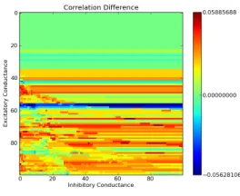
In a simulation run of 10,000 trials, the total correlation was examined with varying excitatory and inhibitory conductances. Typically, the inhibitory conductance has to be one order of magnitude larger than excitatory neurons [93][94], so the range of the excitatory conductance was between 0.0 and 0.1, whereas that of inhibitory conductance was 0.0 and 1.0, with 100 time steps each.

Figure 6.5: Average Correlation Difference

red. We can conclude that the inhibitory conductance plays an important role in correlation: without inhibition, as we saw in the previous model, the correlation decreases as excitatory conductance goes up and as the network starts to fire erratically; with inhibition, the correlation is kept in check.

It seems likely that an increase in the number of excitatory neurons will also have an impact on this. The excitatory-inhibitory ratio varies between 4:1 and 10:1 in the literature [35][93]. Since Vogels & Abbott use the 4:1 ratio and the simplest representation of a binary predicate requires at least 4 neurons, we will choose that ratio.

6.3

Model IIIa: Conductance

The model for the more advanced case where we maintain a 4:1 ratio and rep-resent the predicateLoves for John and Mary is very similar to what we saw in the chapter on the binding problem. Rosenblatt’s example used Triangle, Square, Green and Blue, which is identical to a case where we use John, Mary, Lover and Lovee. Thus, showing binding in this instance of the model solves Jackendoff’s first case of the binding problem.

Figure 6.6: Representation of John, Mary, Lover and Lovee

The representation of a binary predicate John loves Mary then becomes as follows. John and Mary are both connected to the role-encoding neurons, which we have termed Agent and Object. We can stimulate John and Mary, or Agent and Object, and get similar correlation outputs since the connections are recurrent. This is important to stress, because this need not necessarily be the case in advanced models like this.

inhibitors in the models are used as an inhibition pool. Hence, all nodes in the network are connected to the inhibitor pool, which in this case contains only one inhibitory node. The reason for implementing inhibition this way is consistency: the placement of local, lateral and global inhibitors would add a sense of arbitrariness to the models and introduce even more parameters, which we’ve explicitly tried to avoid1_.

Figure 6.7: Correlation Difference for Conductance over John loves Mary

The same test of 10,000 trials was repeated for the network of four excitatory neurons, which shows that the ratio is indeed very important. The plot shows the average correlation difference between the taught bindings. For example, when we teach Agent(John) and Object(Mary), the correlation difference indi-cates how distinguishable these facts are from their alternatives. In other words, it is a measure of correctness of the correlation.

Interestingly, we can see in figure 6.7 that the output is rather peculiar: there appear to be horizontal lines drawn, indicating the the correlation stays the same for some excitatory conductance values, disregarding the inhibitory conductance. It is unclear why this is the case. Luckily, the highest correlation differences occur in places where this pattern is not found, so we can neglect it for our current purposes.

6.4

Model IIIb: Firing Rate

Another important factor in correlation is the firing rates we give to the stimuli. When teaching Agent(John) in the teaching phase, they are given the same firing rates in order to make sure that they bind through spike-time dependent plasticity. In order to avoid overlap between spike-times, the test rates for the trials were all prime numbers below 100, ranging from 2 to 97. The same measure of average correlation difference was used, in order to find an optimum firing rate. The chosen value for excitatory conductance and inhibitory conductance

1_{But see [15] for a thorough discussion of the effect of different types of inhibition on a}

over these trials was one of the optimal values for the previous model, namely an excitatory conductance of 0.085 and inhibitory conductance of 0.55.

Figure 6.8: Correlation Difference for Firing Rate over John loves Mary

The blue and light green colors in figure 6.8 indicate no correlation or neg-ative correlation difference. The dark red in the top right corner shows what values exhibit the highest correlation difference. The optimum rate thus turned out to be the 3rd and 20th prime, giving us 5 and 73 for the firing rates.

6.5

Model IV: Lover and Lovee

With the correct values found for this case, a simple version of the logical model was implemented in Python, so that we can teach the network facts and retrieve the information through queries. A sample run of the trivial programming lan-guage based on the logical model, indicates that the correct results are obtained. The responses are based on a comparison between the alternative possibilities. Because there are only two possibilities per case, no threshold value was neces-sary.

>>>from vb4 import * >>>Loves(john,mary) >>>run()

Done.

>>>Loves(john,mary) True

>>>Loves(mary,john) False

>>>Loves(john,john) False

>>>Loves(mary,mary) False

>>>Loves(X,mary) X = john

Unfortunately, limitations in Brainlab did not allow for the encoding of mul-tiple facts at the same time, but experiments show that it is possible to encode for example Loves(john,mary) and Loves(mary,john) in the same simulation and acquire the correct correlation values to indicate that it is in fact the case that they love each other. Similarly, the correlations that have been found indicate that it is also possible to do something like:

>>>Loves(mary,X) X = none

However, this can only be accomplished when we have determined a way to define a threshold which determines whether or not the correlation is sufficient to show full binding. There are several ways in which this threshold can be implemented, which is an important issue that we will address in the next chapter.

The results obtained for this model show that the network can successfully solve the first of Jackendoff’s problems.

6.6

Model V: Little Big Star

Jackendoff’s second problem is a little harder. First of all, there is the issue of how we measure correlation and between what nodes. When Little and Big both bind to star, but with different firing rates, we will be able to distinguish between them, but what about Agent(Little(star)) and Object(Big(star))?

The easiest way is to compare the total correlation values with each other. That way, when the difference between the correlation of Little(star) and Agent(star) is similar, the network encodes Agent(Little(star)). The similarity between the correlations is indeed apparent from trial runs, as we can see in a sample output with excitatory conductance of 0.085, inhibitory conductance of 0.55 and firing rates of 5 and 73 for the bindings, respectively:

>>>vb5.run()

Little star: 3.53700033637 Big star: 23.657132429 Agent star: 4.48106837019 Object star: 26.3286247906

Figure 6.9: Binding over the Little and the Big Star

similar enough to say that binding has occurred? Since we are using very simple networks, this issue is not very apparent here, but it will become more important once the network is used to encode more facts.

6.7

Model VI: Single Binary Predicate Variable

Binding

Although model IV successfully encodes the predicate Loves(john,mary), that is not the way one would ultimately want to encode a predicate. Whatever way we choose, the possibility of instantiating variables in predicates at a later state is of pivotal importance, because otherwise we will never be able to encode rules using our predicates. One way to do this would be to have multiple constants bound to the roles of the predicate, but further thought shows that this is not enough: we need to be able to re-use variables over different predicates. Something like Loves(X, Y)→ Loves(Y, X) cannot be encoded if we just use the predicate roles. What we need, is instantiable variables that constants can bind to.

Figure 6.10: The Complicated Case Using Actual Variables

6.8

Model VII: Multiple Predicate Variable

Bind-ing

The real test for variable binding is, of course, whether we can in fact re-use the variables. In order to check whether this is the case, we encode two binary predicates, bind variables to their roles and bind constants to these variables. It is important to note that this does not necessarily constitute any particular logical connective, we are just encoding two predicates in the same network. For the sake of clarity, let us call these predicates Loves and Hates, and encode Loves(X,Y) and Hates(Y,X).

Figure 6.11: Two Predicates in One Network

presumably due to the fact that there is a large number of recurrent excitatory connections. Instead of simplifying the model so that it is more likely to reach an equilibrium (for example, by making it a recurrent feed-forward network), an attempt was made to find the optimal values for this network.

Figure 6.12: Correlation Difference over Conductance

A simulation run of 5,000 trials was done, with varying excitatory and in-hibitory conductance values, like in Model IIIa, but only with the higher half of the excitatory values. The plot in figure 6.12 was vertically inverted to make clear that we are not starting from 0, but going up to 0.1 from 0.05. The firing rates were set to 5 and 73. The results show that the difference in correlations is much lower than in the simpler case, as one might expect.

Figure 6.13: Correlation Difference over Firing Rates

using the same firing rates, as was the case in the previous models. It is still possible to encode different facts, but not in such an elegant way.

Chapter 7

Discussion

Variable binding is one important problem, but as goes without saying, it is only the beginning. In order to get clear what any full approach would look like, it is fruitful to highlight some of the features of what has been introduced in the thesis at hand and discuss the obtained results in a little more detail.

7.1

Conception of Logic

To eat something you have to be near it, so the wolf has to ap-proach LRRH. LRRH will scream upon seeing the wolf, because she is scared. The wood-cutters will hear this scream and come to the rescue of the child. The wood-cutters will try to prevent the wolf from attacking LRRH. In doing so they may hurt the wolf physically. The wolf does not want to be hurt physically. So, he decides to wait.

This type of rapid, spontaneous reasoning without conscious effort is what Shastri and Ajjanagadde call reflexive reasoning. Reflexive reasoning is con-trasted with reflective reasoning, which requires reflection, conscious effort and “an overt consideration of alternatives and weighing of possibilities” ([79], p.1). A good example of the reflective kind of reasoning is solving a cross-word puz-zle in the newspaper. If we understand logic as reflexive reasoning–and it is a logical inference after all–a “locus of logic” suddenly becomes a lot more improb-able, if only for the constraints this would put on how rapidly we can reason. Similarly, if such a network would be enormously complex, rapidly and spon-taneously processing the LRRH-inference would be complicated. Thus, there is even an evolutionary argument for this conception of logic, namely that rapid inference is more likely to lead to survival: reflectively drawing the inference “wolf-dangerous-run” would be potentially lethal. It is precisely this kind of logic that we are interested in, because it seems to be an important factor in general human behavior.

More evidence from this conception of logic comes from research in logic and the psychology of reasoning by Stenning and van Lambalgen [87], who have analyzed a range of instances where human reasoning deviates from what classical logic prescribes. They “claim for logic a much wider role in cognition than is customarily assumed, in a complete reversal of the tendency to push logic to the fringes” ([87], p. 347). Stenning and van Lambalgen’s analysis of logic in this context is too sophisticated to explicate in full detail here, but suffice it to say that according to them information processing happens with reference to logical form, which consists of an idealized competence model that is “as such not directly applicable to the real world” ([87], p. 350) in combination with constraints–that is, hypotheses about the world–imposed on that competence model to determine the strictly underdetermined input. Because human beings never have access to all data, they perform a type of non-monotonic reasoning called closed-world reasoning in order to solve reasoning tasks. This process of arriving at logical form is called reasoning to an interpretation. Notably, this type of reasoning does not require awareness, as indeed is illustrated in one of the reasoning tasks that they closely examine (the suppression task).

with setting goals and achieving them, which if it is to be successful requires a form of planning, which in turn requires causal information about the conse-quences of particular actions. Logic, especially non-monotonic logic, lends itself naturally to representing goal-oriented behavior, planning and consequences of actions.

The above considerations are meant to show that, under this conception of logic, it makes perfect sense to implement logic in a biologically plausible net-work. Logical reasoning networks can potentially be all over the brain, as Vogels and Abbott’s results indicate. Reflexive reasoning is something that is the most likely candidate for this type of logical reasoning, as is fundamental cognitive behavior such as goal-orientedness, planning and closed world reasoning, which can all be captured in logic. The reasoning has to be rapid, spontaneous and does not require awareness. Thus, these considerations suggest that any imple-mentation of first-order logic on neural networks should be as simple as possible and reproducible in any neural structure of significant complexity, without ad-hering to a locus of logic.

7.2

Logic Programs and Neural Networks

One may wonder why there has been such a focus on logic programs as the logic of choice. An easy answer would be that this is simply because logic programs have been used successfully in previous work, but that is not sufficient. It is true that logic programs have been used quite successfully, most notably in the works of H¨olldobler and in Stenning and van Lambalgen’s study of human reasoning. However, other logics have also been used, such as Pinkas’ penalty logic [67], to name but one. Luckily, there are other reasons that make logic programs such a suitable candidate, which we will briefly address in what follows.

When artificial intelligence researchers first tried to implement human-like reasoning in artificial agents, they soon discovered that classical logic is far from the best candidate. Human reasoning must be defeasible if we want to be able to deal with the changes in our environment; we must be able to revise our beliefs. As Stenning and van Lambalgen phrase it: “credulous reasoning [where the hearer tries to accommodate the truth of all the speaker’s utterances in deriving an intended model] is best modeled as some form of nonmonotonic logic” ([87], p. 176). This view is closely related to the conception of logic that we discussed previously: classical logic only arises from conscious reflection on human reasoning. Actual human reasoning is much more related to planning and goal-oriented behavior, driven by the evolutionary necessity of rapid reasoning towards a credible model of the environment. This strengthens the case for logic programs as the best candidate to model reflexive reasoning.