uEFS: An efficient and comprehensive
ensemble-based feature selection
methodology to select informative features
Maqbool Ali1,2, Syed Imran Ali1, Dohyeong Kim1, Taeho Hur1, Jaehun Bang1, Sungyoung Lee1*, Byeong Ho Kang2, Maqbool Hussain3
1 Department of Computer Science and Engineering, Kyung Hee University, Yongin, Gyeonggi, Republic of Korea, 2 School of Engineering and ICT, University of Tasmania, Hobart, Tasmania, Australia, 3 Department of Software, Sejong University, Seoul, Gyeonggi, Republic of Korea
Abstract
Feature selection is considered to be one of the most critical methods for choosing appropri-ate features from a larger set of items. This task requires two basic steps: ranking and filter-ing. Of these, the former necessitates the ranking of all features, while the latter involves filtering out all irrelevant features based on some threshold value. In this regard, several fea-ture selection methods with well-documented capabilities and limitations have already been proposed. Similarly, feature ranking is also nontrivial, as it requires the designation of an optimal cutoff value so as to properly select important features from a list of candidate fea-tures. However, the availability of a comprehensive feature ranking and a filtering approach, which alleviates the existing limitations and provides an efficient mechanism for achieving optimal results, is a major problem. Keeping in view these facts, we present an efficient and comprehensive univariate ensemble-based feature selection (uEFS) methodology to select informative features from an input dataset. For the uEFS methodology, we first propose a unified features scoring (UFS) algorithm to generate a final ranked list of features following a comprehensive evaluation of a feature set. For defining cutoff points to remove irrelevant features, we subsequently present a threshold value selection (TVS) algorithm to select a subset of features that are deemed important for the classifier construction. The uEFS methodology is evaluated using standard benchmark datasets. The extensive experimental results show that our proposed uEFS methodology provides competitive accuracy and achieved (1) on average around a 7% increase in f-measure, and (2) on average around a 5% increase in predictive accuracy as compared with state-of-the-art methods.
Introduction
In the domain of data mining and machine learning, one of the most critical problems is the task of feature selection (FS), which pertains to the complexity of the appropriate choosing of features from a larger set of such [1]. FS performs a key role in the (so-called) process of
a1111111111 a1111111111 a1111111111 a1111111111 a1111111111 OPEN ACCESS
Citation: Ali M, Ali SI, Kim D, Hur T, Bang J, Lee S,
et al. (2018) uEFS: An efficient and comprehensive ensemble-based feature selection methodology to select informative features. PLoS ONE 13(8): e0202705.https://doi.org/10.1371/journal. pone.0202705
Editor: Fengfeng Zhou, Jilin University, CHINA
Received: April 30, 2018
Accepted: August 7, 2018
Published: August 28, 2018
Copyright:©2018 Ali et al. This is an open access article distributed under the terms of theCreative Commons Attribution License, which permits unrestricted use, distribution, and reproduction in any medium, provided the original author and source are credited.
Data Availability Statement: All relevant data are
within the paper.
Funding: This research was supported by the MSIT
(Ministry of Science and ICT), Korea, under the ITRC (Information Technology Research Center) support program (IITP-2017-0-01629) supervised by the IITP (Institute for Information &
“knowledge discovery” [2]. Traditionally, this task is performed manually by a human expert, thereby making it more expensive and time-consuming as compared with the use of an auto-matic FS, which has become necessary for the fast-paced digital world of today [3]. FS tech-niques are generally split into the three categories: of filter, wrapper, and hybrid, wherein each technique has capabilities and limitations [3–5]. Popular evaluation methods used for these techniques areinformation-theoretic measures,correlational measures,consistency measures, distance-based measures, andclassification/predictive accuracy. A good FS algorithm can effec-tively filter out unimportant features [6]. Thus, in this regard, a significant amount of research has focused on proposing improved FS algorithms [7–11]; consequently, most of these algo-rithms use one or more of the aforementioned methods for performing FS. However, to date, there remains a lack of a comprehensive framework, which can select features from a given fea-ture set. In order to design such a comprehensive FS methodology, the following two major technical issues must be solved:
1. How to rank the features without the use of any learning algorithm; high computational costs; and the presence of individual statistical biases of state-of-the-art, feature-ranking methods must be considered. In this case, the filter-based, feature-ranking approach is more suitable than the other two approaches (i.e., wrapper and hybrid). Filter-based meth-ods evaluate a feature’s relevance in order to assess its usefulness without using any learning algorithm [1,4]. Filter-based, feature-ranking methods are further split into two subcatego-ries: univariate and multivariate. Univariate filter methods are simple and have high perfor-mance characteristics as compared with the other approaches [12]. However, even though the univariate filter-based methods are considered to be much faster and less computation-ally expensive than wrapper methods [4,13], in reality, each method has its capabilities as well as its limitations. For example, information gain (IG) is a widely acceptable measure for ranking the features [14]; however, IG is biased towards choosing features with a large number of values [15]. Similarly, the chi-squared statistic determines the association between a feature and its target class, but is sensitive to sample size [15]. In addition, gain ratio and symmetrical uncertainty enhances the IG; however, both are biased towards fea-tures with fewer values [16]. Therefore, the designing an efficient feature-ranking approach and the overcoming of the aforementioned limitations compose our first goal.
2. Additionally, how to find a minimum threshold value for retaining important features irre-spective of the characteristics of the dataset must be determined. In this case, for defining cutoff points for removing irrelevant features, a separated validation set and artificially gen-erated features approaches are used [8]; however, it is not clear how to find the threshold for the features’ ranking [17,18]. Research has shown that finding an optimal cutoff value to select important features from different datasets can be problematic [17] and existing methodologies [15,18] required educated guesses to specify a minimum threshold value for retaining important features. Therefore, designing an empirical method to specify a mini-mum threshold value for retaining important features and overcoming the aforementioned limitations is our second target.
Keeping in view these two facts, we have proposed an efficient and comprehensive FS meth-odology, called univariate ensemble-based FS (uEFS), which includes two innovative algo-rithms, unified features scoring (UFS) and threshold value selection (TVS) and which allows for us to select informative features from a given dataset. This study is the extension as well as a detailed review of some of our previous work [19], which proposed a consensus methodology for appropriate FS in order to generate a useful feature subset for the FS task. The UFS algo-rithm generates a final ranked list of features after a comprehensive evaluation of a feature set
Competing interests: The authors have declared
without (1) using any learning algorithm, (2) high computational costs, and (3) the existence of any individual statistical biases of state-of-the-art, feature-ranking methods. The current ver-sion of the UFS has been plugged into a recently developed tool named the data-driven knowl-edge acquisition tool (DDKAT) [19] to assist the domain expert in selecting important features for the data preprocessing task. The DDKAT supports an end-to-end knowledge engineering process for generating production rules from a dataset [19]. The current version of the UFS code and its documentation are freely available and can be downloaded from the GitHub open source platform [20,21]. Similarly, the TVS provides an empirical algorithm to specify a mini-mum threshold value for retaining important features irrespective of the characteristics of the dataset. It selects a subset of features that are deemed important for the classifier construction.
The motivation behind the uEFS is to design and develop an efficient FS methodology for evaluating a feature subset through different angles and to produce a useful reduced feature set. In order to accomplish this aim, this study was undertaken with the following objectives: (1) to design a comprehensive and flexible feature-ranking algorithm to compute the ranks without (a) using any learning algorithm; (b) high computational costs; and (c) any individual statistical biases of state-of-the-art, feature-ranking methods and (2) to identify an appropriate cutoff value for the threshold to select a subset of features irrespective of the characteristics of the dataset with reasonable predictive accuracy.
The key contributions of this research are as follows:
1. The presentation of a flexible approach, called UFS for incorporating state-of-the-art uni-variate filter measures for feature-ranking
2. The proposal of an efficient approach, called TVS, for selecting a cutoff value for the thresh-old in order to select a subset of features
3. The demonstration of a proof-of-concept for the aforementioned techniques, after per-forming extensive experimentation which achieved (1) on average a 7% increase in the f-measure as compared with the baseline approach, and (2) on average a 5% increase in pre-dictive accuracy as compared with state-of-the-art methods.
Related works
This section briefly describes various existing studies related to the FS methodologies to filter out the irrelevant features. This study focused on presenting a comprehensive and flexible FS methodology based on an ensemble of univariate filter measures for the classifier construction. The following includes some relevant FS studies, which contain research surveys and ensem-ble-based approaches for ranking of features as well as identifying a cutoff value for the thresh-old in the domain of FS. Lastly, the overall perspectives of literature reviewed are presented.
that was capable of categorizing existing FS methods based on their common characteristics or their effects on classifiers.
Regarding ensemble-based, feature ranking studies, Rokach et al. [9] and Jong et al. [10] examined the available ensemble-based, feature-ranking approaches to show the improvement in steadiness of FS. Similarly, Slavkov et al. [11] investigated numerous aggregation approaches of feature ranking and observed that aggregating feature rankings produced better results as compared with using the single feature-ranking method. In addition, Prati [8] also obtained bet-ter results using an ensemble feature-ranking approach. In the libet-terature, a hybrid approach by combining the filter and wrapper methods was also presented that is able to eliminate unwanted features by employing a ranking technique [25]. A similar concept to an EFS approach has also been mentioned previously [2,26]. For ensemble feature ranking, two aggregate functions called arithmetic mean and arithmetic median, respectively, were used to rank features [27]. Authors obtained the ranking by arranging the features from the lowest to the highest. Investigators assigned rank 1 to a feature with the lowest feature index and rank M to a feature with the high-est feature index [27]. Similarly, other researchers aggregated several feature rankings to dem-onstrate the robustness of ensemble feature ranking that surges with the ensemble size [10]. Onan and Korukoğlu [12] presented an ensemble-based FS approach, wherein different ranking lists obtained from various FS methods were aggregated. They used a genetic algorithm to pro-duce an aggregate-ranked list, which is a relatively more expensive technique than a weighted aggregate technique. The authors performed experiments of binary class problems, and it was not clear how the proposed method would deal with more complex datasets. Popular filter methods used for the ensemble-based FS approach include IG, gain ratio, chi-squared, symmet-ric uncertainty, one rule (OneR), and ReliefF. Most of the FS methodologies use three or more of the aforementioned methods for performing FS [1,8,15,18,27,28].
With respect to identifying an appropriate cutoff value for the threshold, Sadeghi and Beigy [29] proposed a heterogeneous ensemble-based methodology for feature ranking. These authors used the genetic algorithm to determine the threshold value; however, aθvalue is required to start the process. Moreover, the user is given an additional task of defining the notion of relevancy and redundancy of a feature. Osanaiye et al. [18] combined the output of various filter methods; however, a fixed threshold value i.e. one-third of a feature set, is defined a priori, irrespective of the characteristics of the dataset. Sarkar et al. [15] proposed a technique that aggregates the consensus properties of IG, chi-squared, and symmetric uncertainty FS methods to develop an optimal solution; however, this technique is not comprehensive enough to provide a final subset of features. Hence, a domain expert would still need to make an edu-cated guess regarding the final subset. For defining cutoff points to remove irrelevant features, a separated validation set and artificially generated features approaches can be used [8], though it is not clear how to find the threshold for the features’ ranking [17,18]. Finding an optimal cutoff value to use in selecting important features from different datasets is problematic [17].
Taking into consideration the aforementioned discussion, a significant amount of research [7–12,15,18,24,29] has focused on proposing improved FS methodologies; however, not so much consideration has been paid regarding selecting features from a given feature set in a comprehensive manner. These methodologies either used relatively more expensive tech-niques to select features or required an educated guess to specify a minimum threshold value for retaining important features.
Materials and methods
statistical measures, used for evaluating the performance of the proposed uEFS methodol-ogy, are explained.
Univariate ensemble-based features selection methodology
In the FS process, normally, two steps are required [17]. In the first step, features are typically ranked, whereas, in the second step, a cutoff point is defined to select important features and to filter out the irrelevant features for building more robust machine learning models. In this regard, the proposed UFS algorithm [19] covers the first step of FS, while the TVS algorithm covers the second step.
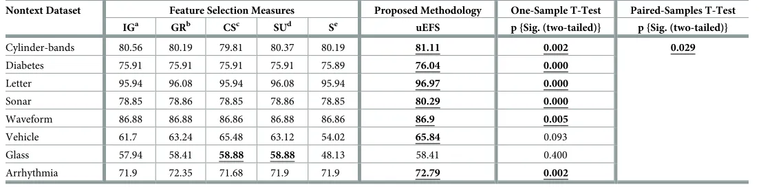
Fig 1shows the functional details of the proposed uEFS methodology, which consists of three major components ofUFS,TVS, andselect features. TheUFScomponent evaluates the feature-set in a comprehensive manner and generates a final ranked list of features. For exam-ple, featuref2has the highest priority, then featuref4, and so on, as shown inFig 1. Similarly,
theTVScomponent defines a cutoff point for selecting important features. Finally, theselect featurescomponent filters out the irrelevant features from the final-ranked list of features based on a cutoff point and selects a subset of features that are deemed as important for the classifier construction. For example,f2,f4,f1,. . .,fn−45is the list of features that were selected
by the proposed uEFS methodology, as shown inFig 1.
Unified features scoring
[image:5.612.121.576.492.698.2]UFS is an innovative feature ranking algorithm that tries to unify various filter-based methods [19] for the purpose of obtaining the final-ranked list of features. In this algorithm, univariate filter measures are employed to assess the usefulness of a selected feature subset in a multidi-mensional manner. These measures are better suited to high-dimultidi-mensional datasets and provide better generalization [4,13]. The UFS algorithm uses theensemble FS(EFS) approach, which has been examined recently by some researchers [2,26]. The EFS, an concept of ensemble learning, obtains a ranked list of features by incorporating the outcomes of different feature-ranking techniques [1,27]. Generally, the intention of the EFS approach is to give an improved estimation to the most favorable subset of features for improving classification performance [2,27,30,31]. As mentioned elsewhere [27], fewer studies have focused on the EFS approach
Fig 1. uEFS methodology.
to enrich the FS itself. Although ensemble-based methodologies have additional computational costs, these costs are affordable due to offering an advisable framework [32]. As discussed pre-viously [27], there are three types of filter approaches:ranking,subset evaluation, and anew FS frameworkthat decouples the redundancy analysis from relevance analysis. The UFS uses a rankingapproach, as it is considered an attractive approach due to its simplicity, scalability, and good empirical success [27,33]. Feature ranking measures the relevancy of the features (i.e., independent attributes) by their correlations to the class (i.e., dependent attribute) and ranks independent attributes according to their degrees of relevance [1]. These values may reveal different relative scales. To neutralize the effect of different relative scales, the UFS rescales the values to the same range (i.e., between 0 and 1) to make it scale-insensitive. For rescaling, the UFS allocates rank 1 to a feature with the highest feature index, as opposed to research that has been done previously [27], which assigned rank 0 to a feature having the top-most feature index. Following that, the UFS orders all scaled ranks in an ascending order and then aggregates them, as it is considered to be an effective technique [8]. The ordered-based, ranking-aggregation method combines the base rankings and considers only the ranks for ordering the attributes [8]. Finally, the UFS computes a mean value to compute weights and priorities of each feature.
UFS is described through Algorithm 1, which takes a dataset (i.e.,D) as input and computes the ranks (scores) of the features after passing through key steps of the algorithm. UFS depends onnunivariate filter-based measures, where the key rationale fornfilter measures is to evalu-ate a feature through different considerations.
Algorithm 1: UFS (D)
Input: D: Input data set (data)
Output: FR− Features Ranks
1 noOfAttrs numAttributes(data) // compute the number of
attributes;
2 / Consider n attribute evaluation measures, also called
univari-ate filter measures (AttrEv1, AttrEv2, AttrEv3,. . ., and AttrEvn) /;
3 / Compute the ranks using each selected measure /;
4 CR1[] computeRanks(data,AttrEv1) //where CR represents computed
ranks;
5 CR2[] computeRanks(data,AttrEv2);
6 CR3[] computeRanks(data,AttrEv3);
7 CRn[] computeRanks(data,AttrEvn);
8 / Compute the scaled ranks of each computed ranks using Algorithm
2 /;
9 scaledRanks1[] scaleRanks(CR1) // invoke Algorithm 2;
10 scaledRanks2[] scaleRanks(CR2) // invoke Algorithm 2;
11 scaledRanks3[] scaleRanks(CR3) // invoke Algorithm 2;
12 scaledRanksn[] scaleRanks(CRn) // invoke Algorithm 2;
13 / Compute the combined sum of all computed ranks /;
14 combinedranksSum 0;
15 combinedRanks[];
16 for 8 noOfAttrs2 D do
17 / For each attribute, compute the combined rank by adding all
computed scaled ranks /;
18 combinedRanksi
Xn
j¼1
scaledRanksji //where n represents the number of
filter measures;
19 combinedranksSum= combinedranksSum+ combinedRanksi;
20 end
21 / Rank the list in ascending order /;
23 / Compute the score, weight, and priority of each attribute /;
24 for 8 noOfAttrs2 D do
25 attrScoresi combinedRanksi/n //where n represents number of
fil-ter measures;
26 attrWeightsi combinedRanksi/combinedranksSum;
27 attrPrioritiesi attributesScoresi attributesWeightsi;
28 / Assign an index (Rank ID) on ascending order to each
attri-bute based on its priority value /;
29 FR[] assignRank(attrPrioritiesi);
30 end
31 return FR: features ranks
Algorithm 2: Scaling the Computed Ranks (CR) Input: CR: Input computed ranks (ranks)
Output: SR− Scaled Ranks
1 smallest ranks0;
2 largest ranks0;
3 for 8 noOfAttrs 2 CR do
4 if ranki > largest then
5 largest ranki;
6 else
7 if ranki < smallestthen
8 smallest ranki
9 end
10 end
11 end
12 min smallest;
13 max largest;
14 SR[] (ranks− min)/(max − min);
15 return SR: scaled ranks
In Algorithm 1, the first step is to compute the number of features from a given dataset. Then, in the second step, each feature in a dataset can be ranked usingnnumber of univariate filter-based measures, as shown in Line 4 to Line 7 of Algorithm 1. After that, Algorithm 2 was used to scale (normalize) all computed ranks using the first filter measure. This step was repeated for the remaining (n−1) measures as well as shown in Line 9 to Line 12. After the evaluation and scaling process, ranks aggregations were performed, as shown in Line 18 of Algorithm 1. Later, the comprehensive score as well as the weightage of each feature were computed, as shown in Line 25 and Line 26 of Algorithm 1. Finally, based on the contribution (i.e., individual measure score and relative weightage), a priority value of each feature was computed. This priority value of a feature was further utilized for ranking and feature subset selection.
For the proof-of-concept, five univariate filter-based measures—namely, IG, gain ratio, symmetric uncertainty, chi-squared, and significance [1,8,19,27,28]—were used to explain the process of the proposed unified features scoring algorithm. The reasons for selecting these five measures are described elsewhere [19]. Using these five filter measures, the process of the UFS is depicted inFig 2. This process is also explained through an example.
Threshold value selection
TVS is explained through Algorithm 3. This algorithm takesndatasets (i.e.,D) andm classi-fiers (i.e.,C) as input and sequentially passes them through mandatory steps of the algorithm to find the cutoff value from a predictive accuracy graph.
Algorithm 3: TVS (D,C)
Input: D − (d1, d2,. . .,dn) // set of n datasets with varying
complexities
C − (c1, c2,. . .,cm) // set of m machine learning classifiers Output: V − cutoff value
1 initialization; 2 for di in D do
3 di computeFeatureRank(di) // rank each feature;
4 di sortByRankASC(di) // sort features by rank in ASC;
5 end
6 P 100;
7 for di in D do 8 while P 5 do
9 k sizeOf(di) (p/100) // compute partition size;
10 Acc newSet() // initialize empty set;
11 for ci in C do;
12 Pacc predictiveAccuracy(ci, topKFeatures(di, k));
13 Acc.add(Pacc) // add accuracy to set;
14 end
15 AVGacc computeAVG(Acc) // compute average accuracy;
16 G Plot(AVGacc, k) // plot the average point;
17 P P − 5 // decrease the partition size by 5;
18 end
19 end
20 V getCutoffValue(G);
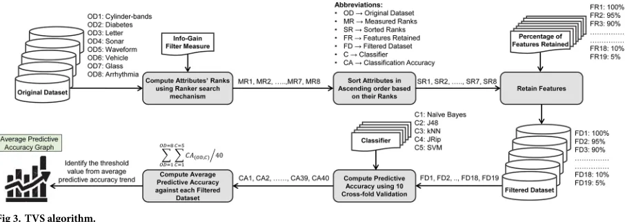
[image:8.612.119.577.78.250.2]In Algorithm 3, first consider thennumber of benchmark datasets having varying com-plexities. After that, compute the feature ranks using a ranker search mechanism and then sort them in an ascending order, as shown in Line 3 and Line 4 of Algorithm 3. Then, partition each dataset into different chunks (filtered datasets) from 100% to 5% features retained. Once filtered datasets are created, then considermnumber of classifiers from various classifiers cate-gories/families having varying characteristics (wheremn) and feed each filtered dataset to these classifiers as shown in Line 6 and Line 11 of Algorithm 3. Following this, record predic-tive accuracies of these classifiers to each chunk of dataset partitioning using 10-fold cross vali-dation approach (Line 12). Later, compute the average predictive accuracy of all classifiers as
Fig 2. UFS algorithm [19].
well as datasets against each chunk of dataset partitioning (Line 15). Finally, plot all computed average predictive accuracies against each chunk of dataset partitioning (Line 16) and identify the cutoff value from the plotted graph (Line 20).
For the proof-of-concept, eight datasets of varying complexities were used to explain the process of the proposed threshold selection algorithm. The process of threshold value selection is depicted inFig 3.
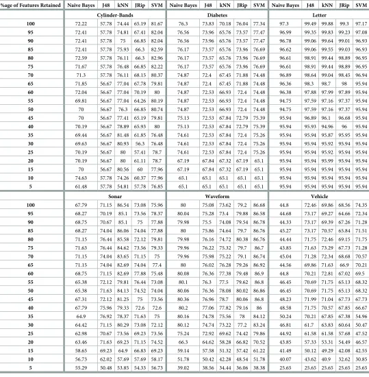
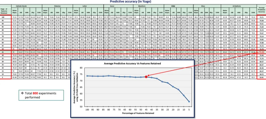
As depicted inFig 3, each dataset (Cylinder-bands,Diabetes,Letter,Sonar,Waveform, Vehicle,Glass,Arrhythmia) was fed to theIGfilter measure for computing attributes’ ranks. Then, all measured ranks of attributes of each dataset were sorted in ascending order. After-wards, each dataset was partitioned into different chunks (filtered datasets) from 100% to 5% features retained, e.g., in case of an 80% chunk, the dataset retains nearly 80% of the highly ranked features, while 20% of the features, which are below the rank, are discarded. Each fil-tered dataset was fed to five well-known classifiers from various classifier categories/families having varying characteristics [e.g., naive Bayes from theBayescategory, J48 from theTrees category, k-nearest neighbors (kNN) from theLazycategory, JRip from theRulescategory, and support vector machine (SVM) from theFunctionscategory] and, using a10-fold cross-validationapproach [8], predictive accuracies of these classifiers were recorded to each chunk of dataset partitioning, as illustrated inTable 1. Finally, an average predictive accuracy of all classifiers as well as the datasets against each chunk of dataset partitioning were com-puted. The main intuition of this process is to identify an appropriate chunk value that pro-vides reasonable predictive accuracy and considerably reduces the dataset as well. Through empirical evaluation, it was found that a 45% chunk provided a reasonable threshold value of feature subset selection (Fig 4).
State-of-the-art feature selection methods for comparing the performance of the pro-posed univariate ensemble-based feature selection methodology. In this study, both
sin-gle-FS methods—namely, IG, gain ratio, symmetric uncertainty, chi-squared, significance, OneR, Relief, ReliefF, and decision rule-based FS (DRB-FS) —and ensemble-based FS methods such as gain-ratio—chi-squared (GR-χ2), the Borda method, and ensemble-based multifilter FS (EMFFS) method were used as state-of-the-art FS methods for comparing the performance of the proposed uEFS methodology [1,8,15,18,19,27,28]. Each of the FS meth-ods is defined as follows:
[image:9.612.123.576.77.238.2]IG is an information theoretic as well as a symmetric measure and is one of the popular measures for FS. It is calculated based on a feature’s contribution in enhancing information
Fig 3. TVS algorithm.
Table 1. Predictive accuracy (in %age) of classifiers using benchmark datasets.
%age of Features Retained Naive Bayes J48 kNN JRip SVM Naive Bayes J48 kNN JRip SVM Naive Bayes J48 kNN JRip SVM
Cylinder-Bands Diabetes Letter
100 72.22 57.78 74.44 65.19 81.67 76.3 73.83 70.18 76.04 77.34 97.3 99.49 99.88 99.3 97.17
95 72.41 57.78 74.81 67.41 82.04 76.56 73.96 65.76 73.57 77.47 96.99 99.35 99.83 99.23 97.08
90 72.41 57.78 75 66.85 82.04 76.56 73.96 65.76 73.57 77.47 96.78 99.06 99.64 99.01 96.93
85 72.41 57.78 75.93 66.3 82.59 76.17 73.57 65.76 73.96 76.69 96.62 99.06 99.55 99.03 96.93
80 72.59 57.78 76.11 66.3 82.96 76.17 73.57 65.76 73.96 76.69 96.61 98.91 99.44 98.89 96.95
75 71.67 57.78 76.48 66.85 82.22 76.17 73.57 65.76 73.96 76.69 96.61 98.91 99.44 98.89 96.95
70 71.3 57.78 76.11 68.15 80.37 74.87 72.4 67.45 71.88 74.48 96.89 98.64 99.04 98.45 96.94
65 71.85 56.67 77.04 67.78 79.81 74.87 72.4 67.45 71.88 74.48 96.36 98.3 98.7 98 95.94
60 72.04 56.67 77.04 70.19 80 74.87 72.53 66.93 72.4 74.48 96.38 97.88 97.99 97.89 95.94
55 69.81 56.67 77.04 64.26 80.19 74.87 72.53 66.93 72.4 74.48 94.75 97.59 97.16 97.37 95.94
50 70 56.67 76.3 66.85 80.74 74.87 72.53 66.93 72.4 74.48 94.75 97.59 97.16 97.37 95.94
45 70 56.67 77.41 65.19 79.81 75.13 72.53 67.84 72.79 75.39 95.94 96.89 96.1 96.68 95.94
40 70.19 56.67 78.89 65.93 80 75.13 72.53 67.84 72.79 75.39 95.94 95.93 94.96 96 95.94
35 69.44 56.67 81.48 61.85 76.48 74.61 72.53 67.84 72.4 75.26 95.94 95.94 95.87 95.95 95.94
30 69.63 56.67 80.93 56.3 76.48 74.61 72.53 67.84 72.4 75.26 95.94 95.94 95.92 95.94 95.94
25 70.19 56.67 80 57.41 78.7 74.61 72.53 67.84 72.4 75.26 95.94 95.94 95.92 95.94 95.94
20 70.19 56.67 80 61.11 78.7 67.19 67.84 67.32 67.19 65.1 95.94 95.94 95.99 95.94 95.94
15 70 56.67 80.56 60 77.96 67.19 67.84 67.32 67.19 65.1 95.94 95.94 95.94 95.94 95.94
10 74.63 57.78 74.26 60.37 77.96 65.1 65.1 65.1 65.1 65.1 95.94 95.94 95.94 95.94 95.94
5 61.48 57.78 54.81 57.78 76.85 65.1 65.1 65.1 65.1 65.1 95.94 95.94 95.94 95.94 95.94
Sonar Waveform Vehicle
100 67.79 71.15 86.54 73.08 75.96 80 75.08 73.62 79.2 86.68 44.8 72.46 69.86 68.56 74.35
95 68.27 70.19 85.1 73.56 78.37 80.04 75.28 73.4 79.88 86.58 44.68 73.17 69.27 64.66 72.34
90 68.75 70.67 85.1 75 77.88 79.98 75.5 74.08 79.54 86.78 44.33 73.17 69.39 67.26 71.28
85 68.27 74.04 86.06 74.04 77.88 80 75.86 74.64 79.7 86.76 45.27 73.17 70.57 65.84 71.51
80 71.15 76.44 85.58 72.12 79.81 79.98 76.16 74.72 80.38 86.76 44.44 71.75 72.46 69.15 71.75
75 71.63 76.44 84.62 73.56 79.33 79.96 76.22 75.32 79.7 86.7 43.85 71.63 73.29 67.73 71.28
70 71.15 74.04 83.65 71.15 75 79.96 75.98 75.22 79.1 86.74 45.04 71.28 72.34 68.68 70.57
65 71.15 74.04 82.69 74.04 77.4 80 76.02 76.28 79.26 86.92 44.56 69.86 71.63 66.9 70.21
60 68.75 71.15 82.69 77.88 75.48 80.08 76.36 77.38 79.48 86.9 44.8 70.21 72.81 67.02 69.5
55 65.38 72.12 79.81 76.44 73.08 80.1 76.3 77.5 79.62 86.8 46.45 70.69 71.75 65.13 68.32
50 65.38 71.63 84.13 74.52 74.04 80.06 76.36 78.08 80.02 86.86 46.45 70.69 71.75 65.13 68.32
45 67.31 72.12 81.25 75 73.56 80.36 76.96 78.7 80.06 86.8 48.23 71.99 71.04 67.73 67.73
40 67.79 75.96 79.33 72.6 72.6 80.2 77.06 77.82 79.16 86 48.58 71.75 70.57 67.85 66.67
35 64.9 76.92 78.37 71.63 75 80.16 74.78 75.56 78 84.12 50.24 70.21 67.85 67.38 54.96
30 64.42 71.15 80.29 73.08 72.12 80.12 74.74 73.22 77.2 83.24 46.81 61.7 63.83 60.64 50.47
25 62.98 70.67 73.56 69.23 73.56 75.24 72.92 69.62 74.42 79.86 44.92 61.58 61.58 57.68 47.52
20 63.46 71.63 69.23 71.15 74.52 66.3 64.62 58.28 66.82 70.52 43.85 57.33 53.31 54.49 46.57
15 58.65 69.23 64.9 66.83 69.23 59.14 57.58 51.32 57.42 61.22 41.49 50.12 49.29 42.08 42.55
10 56.73 62.02 57.69 57.69 58.17 51.78 50.42 42.28 48.54 51.78 40.07 43.62 40.9 32.62 30.85
5 55.29 50.48 53.85 54.33 56.73 39.02 38.56 34.44 36.06 38.38 25.65 25.65 25.65 25.65 25.65
about the target class label. An equation for IG is given as follows [14]:
IGðAÞ ¼InfoðDÞ InfoAðDÞ ð1Þ
whereIG(A)is the IG of an independent feature or attributeA,Info(D)is the entropy of the entire dataset, andInfoA(D) is the conditional entropy of attributeAoverD.
Table 1. (Continued)
%age of Features Retained Naive Bayes J48 kNN JRip SVM Naive Bayes J48 kNN JRip SVM Naive Bayes J48 kNN JRip SVM
Glass Arrhythmia
100 48.6 66.82 70.56 68.69 56.07 62.39 64.38 52.88 70.8 70.13
95 50.47 67.29 77.1 66.36 51.87 63.05 65.27 52.65 69.69 70.35
90 50.47 67.29 77.1 66.36 51.87 61.95 63.5 51.77 68.58 69.91
85 47.66 70.09 77.1 62.15 51.87 60.84 61.95 51.33 70.13 70.35
80 47.66 70.09 77.1 62.15 51.87 60.4 64.38 51.77 69.91 71.02
75 46.26 72.9 73.36 60.28 51.87 59.51 64.82 51.11 68.81 70.8
70 46.26 72.9 73.36 60.28 51.87 61.28 63.27 50.22 69.47 72.12
65 47.66 71.5 72.9 62.62 51.4 61.95 61.95 49.34 68.81 71.46
60 47.66 71.5 72.9 62.62 51.4 59.96 61.95 50.22 67.26 70.13
55 50.93 74.3 74.77 64.49 51.4 59.73 63.27 50.22 70.58 68.14
50 50.93 74.3 74.77 64.49 51.4 59.73 63.27 49.56 65.49 69.47
45 50.93 74.3 74.77 64.49 51.4 60.62 63.72 49.78 69.47 68.58
40 46.73 66.36 72.9 67.76 46.73 61.5 62.61 48.23 68.36 69.25
35 46.73 66.36 72.9 67.76 46.73 62.17 64.38 47.79 68.14 68.36
30 43.46 63.55 57.01 60.28 35.51 59.07 61.5 45.35 65.93 63.94
25 43.46 63.55 57.01 60.28 35.51 59.29 61.95 44.03 65.93 63.27
20 35.98 54.67 47.2 52.8 35.51 61.5 61.95 46.24 66.15 63.27
15 35.98 54.67 47.2 52.8 35.51 63.05 61.5 52.65 65.04 61.73
10 35.51 35.51 35.51 35.51 35.51 63.05 54.2 52.21 65.04 61.5
5 35.51 35.51 35.51 35.51 35.51 60.18 49.34 47.12 61.5 61.5
[image:11.612.33.574.92.374.2]https://doi.org/10.1371/journal.pone.0202705.t001
Fig 4. An average predictive accuracy graph using the 10-fold cross-validation technique for threshold value identification.
[image:11.612.123.574.487.689.2]Gain ratiois considered to be one of the disparity measures that provides normalized score to enhance the IG result. This measure utilizes the split information value that is given as fol-lows [14]:
SplitInfoAðDÞ ¼ Xv
j¼1
jDjj
jDjlog2
jDjj
jDj ð2Þ
whereSplitInforepresents the structure ofvpartitions. Finally, gain ratio is defined as follows [14]:
GainRatioðAÞ ¼IGðAÞ=SplitInfoðAÞ ð3Þ
Chi-squaredis a statistic measure that computes the association between the attributeAand its class or categoryCi. It helps to measure the independence of an attribute from its class. It is
defined as follows [14]:
CHIðA;CiÞ ¼
N ðF1F4 F2F3Þ 2
ðF1þF3Þ ðF2þF4Þ ðF1þF2Þ ðF3þF4Þ
ð4Þ
CHImaxðAÞ ¼maxiðCHIðA;CiÞÞ ð5Þ whereF1,F1,F3, andF4represent the frequencies of occurrence of bothAandCi,Awithout
Ci,CiwithoutA, and neitherCinorA, respectively, whileNrepresents the total number of
attributes. A zero value of CHI indicates that bothCiandAare independent.
Symmetric uncertaintyis an information theoretic measure to assess the rating of con-structed solutions. It is a symmetric measure and is expressed by the following equation [34]:
SUðA;BÞ ¼ 2IGðAjBÞ
HðAÞ þHðBÞ ð6Þ
whereIG(A|B) represents the IG computed by an independent attributeAand the class-attri-buteB. WhileH(A)andH(B)represent the entropies of the attributesAandB.
Significanceis a real-valued, two-way function used to assess the worth of an attribute with respect to a class attribute [35]. The significance of an attributeAiis denoted byσ(Ai), which is
computed by the following equation:
sðAiÞ ¼
AEðAiÞ þCEðAiÞ
2 ð7Þ
whereAE(Ai) represents the cumulative effect of all possible attribute-to-class associations of
an attributeAi, which are computed as follows:
AEðAiÞ ¼ 1=k X
r¼1;2;...;k Wir
!
1:0 ð8Þ
wherekrepresents the different values of the attributeAi.
Similarly,CE(Ai) captures the effect of change of an attribute value by the changing of a
class decision and represents the association between the attributeAiand various class
deci-sions, which is computed as follows:
CEþ ðAiÞ ¼ ð1=mÞ
X
j¼1;2;...;m Ai
j !
wheremrepresents the number of classes and + (Ai) depicts the class-to-attribute association
of the attributeAi.
OneR is the rule-based method to generate a set of rules, which test one particular attribute. The details of this method can be found elsewhere [36].
Relief[37] andReliefF[38] are distance-based methods to estimate the weightage of a fea-ture. The original Relief method deals with discrete and continuous attributes; it does not sup-port attempts to deal with incomplete data and is limited to application in two-class problems. ReliefF is an extension of the Relief method that covers the limitations of the Relief method. The details of these methods can be found elsewhere [37,38].
DRB-FS is a statistical measure to eliminate all irrelevant and redundant features. It allows one to integrate domain-specific definitions of feature relevance, which are based on high, medium, and low correlations that are measured using Pearson’s correlation coefficient, which is computed as follows [29,39]:
rXY ¼
P
ðxi xÞðyi yÞ
ðn 1ÞSXSY
ð10Þ
wherexandyrepresent the sample means andSXandSYare the sample standard deviations
for the featuresXandY, respectively. Here,nrepresents the sample size.
GR-χ2is an ensemble ranking method that simply adds together the computed ranks of the gain ratio and chi-squared methods [29].
TheBorda methodis a position-based, ensemble-scoring mechanism that aggregates rank-ing results of features from multiple FS techniques [15]. The final rank of a feature is computed as follows:
scorefinal ¼ Xn
i¼1
scoreposði;jÞ ð11Þ
wherenrepresents the total number of FS techniques andpos(i,j) is thejthposition of a feature ranked by theithFS technique.
EMFFS is an ensemble FS method that combines the output of four filter methods— namely, IG, gain ratio, chi-squared, and ReliefF—in order to obtain an optimum selection [18].
Statistical measures for evaluating the performance of the proposed univariate ensem-ble-based feature selection methodology. In this study, precision, recall, f-measure, and the
percentage of correct classification were used as evaluation criteria for FS accuracy [8,12,15,
18,29,40]; second for processing speed; and third as part of a10-fold cross-validation tech-nique for computing predictive accuracy to evaluate the performance of machine learning methods or schemes [8,12,18,41–43].
In order to compute the statistical measures (i.e., precision, recall, f-measure, and the per-centage of correct classification), the following four measures were required:
• True positives(TP) represents the correctly predicted positive values (actual class = yes, pre-dicted class = yes)
• True negatives(TN) represents the correctly predicted negative values (actual class = no, pre-dicted class = no)
• False negatives(FN) represents a different contradiction between the actual and predicted classes (actual class = yes, predicted class = no)
Joshi [44] defined these measures as follows:
“Accuracyis a ratio of correctly predicted observations to the total observations,” which is computed as follows:
Accuracy¼ TPþTN
TPþFPþFNþTN ð12Þ
“Precisionis the ratio of correctly predicted positive observations to the total predicted posi-tive observations,” which is computed as follows:
Precision¼ TP
TPþFP ð13Þ
“Recallis the ratio of correctly predicted positive observations to all observations in the actual class—yes,” which is computed as follows:
Recall¼ TP
TPþFN ð14Þ
“F-measureis the weighted average of Precision and Recall,” which is computed as follows:
F measure¼2 ðRecallPrecisionÞ
ðRecallþPrecisionÞ ð15Þ
Experimental results of the threshold value selection algorithm
This section demonstrates the results of the proposed TVS algorithm. The purpose is to inter-pret as well as comment on the results obtained from the experiments.
Table 1presents the predictive accuracies of eight datasets (i.e.,Cylinder-bands,Diabetes, Letter,Sonar,Waveform,Vehicle, Glass, andArrhythmia) against five classifiers (naive Bayes, J48,kNN,JRip, andSVM) with varying threshold values from 100 to 5. In this table, predictive accuracies are recorded as percentages, which were determined by the10-fold cross-validation technique, whereas, each threshold value represents the percentage of features retained. After recording the predictive accuracies, the average predictive accuracy of all classifiers as well as datasets against each threshold value was computed, which is shown inFig 4. This figure depicts the summarized effects of different threshold values on the predictive accuracy of the datasets noted inTable 1.
Furthermore, predictive accuracies using training examples of the aforementioned eight datasets were also recorded against the same five classifiers with varying threshold values from 100 to 5. After recording the predictive accuracies, again, an average predictive accuracy of all classifiers as well as datasets against each threshold value was computed, which is shown in
Fig 5.
Evaluation of the univariate ensemble-based feature selection
methodology
The evaluation phase of any methodology has a key role in investigating the worth of any pro-posed method. This section covers the experimental setup as well as execution to evaluate the proposed uEFS methodology with state-of-the-art FS methods. The purpose was to check the impact of the proposed methodology on FS suitability in terms of features’ ranking according to the precision, recall, f-measure, and predictive accuracy performance measure factors.
Experimental setup
For holistic understanding, two studies were performed to evaluate the uEFS methodology by involving nontext and text benchmark datasets. In each study, the methodology was com-pared with the state-of-the-art FS methods using precision, recall, f-measure, and predictive accuracy performance measure factors. The motivation behind comparing the results achieved with the text and nontext datasets was to check the scalability of the proposed uEFS methodol-ogy from small- to high-dimensional data, wheredimensionrepresents the number of attri-butes or features.
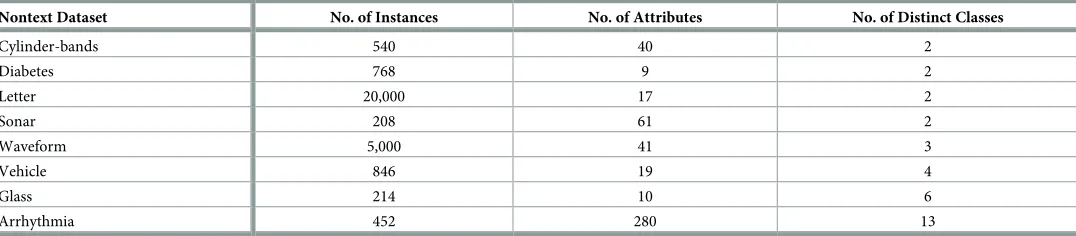
For thefirst study, eight nontext benchmark datasets of varying complexity (i.e., small to medium size and binary to multiclass problems), were chosen, includingCylinder-bands, Dia-betes,Letter,Sonar,Waveform,Vehicle, Glass, andArrhythmia, as shown in theTable 2. These datasets were collected from the openML repository available athttp://www.openml.org/.
[image:15.612.117.580.72.298.2]For thesecond study, the following four text datasets of varying complexity were selected: MiniNewsGroups(http://kdd.ics.uci.edu/databases/20newsgroups/20newsgroups.html), Course-Cotrain(http://www.cs.cmu.edu/afs/cs.cmu.edu/project/theo-51/www/co-training/ data/course-cotrain-data.tar.gz),Trec05p-1(https://plg.uwaterloo.ca/gvcormac/treccorpus/), andSpamAssassin(http://csmining.org/index.php/spam-assassin-datasets.html). These data-sets are in text form and, to apply the feature-ranking algorithms on these datadata-sets, there is a need to preprocess the text data into a structured form. In order to perform text preprocessing, the following tasks were completed:
Fig 5. An average predictive accuracy graph using training datasets for threshold value identification.
1. Remove Hypertext Markup Language tags from web documents, sender as well as receiver information from e-mail documents, URLs, etc.
2. Eliminate pictures and email attachments from the documents
3. Tokenize the documents
4. Remove the noninformative terms like stopwords from the contents
5. Perform the term stemming task
6. Eliminate the low-length terms whose length is less than or equal to 2
[image:16.612.37.575.89.207.2]7. Finally, generate the feature vectors representing document instances by computing the Term Frequency—Inverse Document Frequency weights.
Table 3shows the characteristics of the structured form of the text datasets. These datasets also have varying complexity (i.e., small to medium size and binary to multiclass problems).
To select a suitable classifier for assessing the proposed uEFS methodology, initially, five well-known classifiers were used: naive Bayes, J48, kNN, JRip, and SVM [8,12,15,18,29,40,
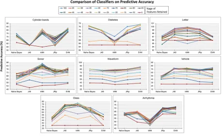
45,46]. Using each classifier, predictive accuracy was measured with a varying percentage of features retained values from 100 to 5, as illustrated inFig 6. The pictorial results show that, of the five classifiers, SVM and kNN tended to perform best with regard to the above-men-tioned datasets.Fig 6shows the four datasets—namelyCylinder-bands,Diabetes,Waveform, andArrhythmia—on which SVM performed better. Likewise,Fig 6shows the three datasets (Letter,Sonar, andGlass) on which kNN performed best. In recent years, the SVM classifier has been considered as a dominant tool for dealing with classification problems in a wide range of applications [45] and is largely preferred over other classification methods [46].
Keeping in view with theFig 6results and state-of-the-art classifier considerations, finally, the SVM classifier was used to assess the proposed uEFS methodology, as it tends to outper-form the F-measures and predictive accuracies for the benchmark datasets [29,45]. Further,
Table 2. Selected nontext datasets’ characteristics.
Nontext Dataset No. of Instances No. of Attributes No. of Distinct Classes
Cylinder-bands 540 40 2
Diabetes 768 9 2
Letter 20,000 17 2
Sonar 208 61 2
Waveform 5,000 41 3
Vehicle 846 19 4
Glass 214 10 6
Arrhythmia 452 280 13
[image:16.612.36.577.629.697.2]https://doi.org/10.1371/journal.pone.0202705.t002
Table 3. Selected text datasets’ characteristics.
Text Dataset No. of Features No. of Documents No. of Distinct Classes
MiniNewsGroups 27,419 1,600 4
Course-Cotrain 13,919 1,051 2
Trec05p-1 12,578 62,499 2
SpamAssassin 9,351 3,000 2
theSMOregfunction (SVM with sequential minimum optimization) of the SVM classifier was used, which is an improved version of the SVM [47].Table 4shows the parameters of the selected classifier.
For comparison purposes, a standard open-source implementation of this classifier was uti-lized as provided by theWaikato Environment for Knowledge Analysis(WEKA) available at
http://weka.sourceforge.net/doc.dev/. Using open-source implementation, a method in Java language was written, which computes precision, recall, f-measure, and predictive accuracy of this classifier using the 10-fold cross-validation technique.
Finally, to compare the computational cost, the performance speed of the proposed meth-odology as well as state-of-the-art methods were measured on a system having the following specifications:
• Processor: Intel (R) Core (TM) i5-2500 CPU @ 3.30 GHz
• Installed memory (RAM): 16.0 GB
• System type: 64-bit operating system
Experimental execution
[image:17.612.120.578.78.358.2]For thefirst study, a comparison was made between the proposed uEFS methodology and the aforementioned five univariate filter measures, which were used for the proof-of-concept.
Fig 6. Predictive accuracies of classifiers against benchmark datasets with varying percentages of retained features.
https://doi.org/10.1371/journal.pone.0202705.g006
Table 4. Selected classifier parameters.
Classifier Function Kernel Type Epsilon Tolerance Exponent Random Seed
SVM SMO Polynomial 1.0E-12 0.001 1 1
Fig 7depicts the difference of the f-measure of the proposed uEFS methodology with each FS measure, which is used in the uEFS methodology. It can be deduced from the results, shown in
Fig 7, that the proposed methodology provides competitive results as compared with state-of-the-art FS measures.
For comparison purposes, computed precision and recalls were also used, as recorded in Tables5and6. The results of these two tables also reveal that the proposed methodology pro-vides better results. The proposed uEFS methodology yields significant precision and recall on all nontext datasets exceptGlassagainst all existing feature selection measures. On recall com-parison, the closest competitors to the uEFS methodology were IG, gain ratio, and symmetrical uncertainty measures, which achieved a similar recall of 0.869 with theWaveformdataset. Regarding the other datasets, the existing measures achieved a much lower recall as compared with the uEFS. Similarly, with respect to the precision comparison, the chi-squared and sym-metrical uncertainty remained the closest competitors to the uEFS for theGlassdataset. For the rest of the datasets, the uEFS outperformed the existing FS measures with a significant difference.
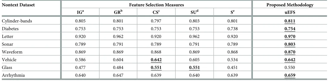
[image:18.612.118.581.84.205.2]A comparison was also made between the predictive accuracies of the uEFS methodology and the five aforementioned univariate filter measures.Table 7illustrates the comparison of
Fig 7. Comparisons of F-measure with existing FS measures.
[image:18.612.33.581.493.629.2]https://doi.org/10.1371/journal.pone.0202705.g007
Table 5. Comparisons of average classifier precision with existing FS measures.
Nontext Dataset Feature Selection Measures Proposed Methodology
IGa GRb CSc SUd Se uEFS
Cylinder-bands 0.805 0.801 0.797 0.803 0.801 0.811
Diabetes 0.753 0.753 0.753 0.753 0.738 0.754
Letter 0.920 0.962 0.920 0.962 0.920 0.970
Sonar 0.789 0.791 0.789 0.791 0.789 0.803
Waveform 0.869 0.869 0.868 0.869 0.868 0.870
Vehicle 0.586 0.604 0.642 0.605 0.534 0.642
Glass 0.477 0.484 0.551 0.551 0.451 0.550
Arrhythmia 0.640 0.647 0.639 0.640 0.639 0.659
a
IG: information gain,
b
GR: gain ratio,
c
CS: chi-squared,
d
SU: symmetrical uncertainty,
e
S: significance
the predictive accuracy of the uEFS methodology with the five FS measures that are used in the uEFS methodology. It can be observed from theTable 7results that the proposed methodology provides competitive results as compared with existing FS measures. Similarly, it can also be seen from the results shown inFig 7and Tables5,6, and7, respectively, that, in terms of f-measure, precision, recall, and predictive accuracy, the proposed methodology did not per-form better than existing FS measures on theGlassdataset due to having a small size of data, multiple classes, and imbalanced class characteristics.
[image:19.612.32.581.90.226.2]The result ofone-sample t-testandpaired-samples t-testis also illustrated inTable 7. The purpose of performing this test was to determine whether the values obtained from the pro-posed uEFS methodology were significantly different from the values obtained from existing
Table 6. Comparisons of average classifier recall with existing FS measures.
Nontext Dataset Feature Selection Measures Proposed Methodology
IGa GRb CSc SUd Se uEFS
Cylinder-bands 0.806 0.802 0.798 0.804 0.802 0.811
Diabetes 0.759 0.759 0.759 0.759 0.758 0.760
Letter 0.959 0.961 0.959 0.961 0.959 0.970
Sonar 0.788 0.789 0.788 0.789 0.788 0.803
Waveform 0.869 0.869 0.868 0.869 0.868 0.869
Vehicle 0.617 0.632 0.655 0.631 0.540 0.658
Glass 0.579 0.584 0.589 0.589 0.481 0.584
Arrhythmia 0.719 0.723 0.717 0.719 0.719 0.728
a
IG: information gain,
b
GR: gain ratio,
c
CS: chi-squared,
d
SU: symmetrical uncertainty,
e
S: significance
https://doi.org/10.1371/journal.pone.0202705.t006
Table 7. Comparisons of predictive accuracy (in %age) of the uEFS with existing FS measures.
Nontext Dataset Feature Selection Measures Proposed Methodology One-Sample T-Test Paired-Samples T-Test
IGa GRb CSc SUd Se uEFS p {Sig. (two-tailed)} p {Sig. (two-tailed)}
Cylinder-bands 80.56 80.19 79.81 80.37 80.19 81.11 0.002 0.029
Diabetes 75.91 75.91 75.91 75.91 75.89 76.04 0.000
Letter 95.94 96.08 95.94 96.08 95.94 96.97 0.000
Sonar 78.85 78.86 78.85 78.86 78.85 80.29 0.000
Waveform 86.88 86.88 86.86 86.88 86.86 86.9 0.005
Vehicle 61.7 63.24 65.48 63.12 54.02 65.84 0.093
Glass 57.94 58.41 58.88 58.88 48.13 58.41 0.400
Arrhythmia 71.9 72.35 71.68 71.9 71.9 72.79 0.002
a
IG: information gain,
bGR: gain ratio, c
CS: chi-squared,
d
SU: symmetrical uncertainty,
eS: significance
[image:19.612.32.585.488.624.2]FS measures. For performing this test against each dataset, FS measures’ values were consid-ered as sample data and the uEFS value was designated as a test value, which is a known or hypothesized population mean. For example, in the case of theCylinder-bandsdataset, 81.11 (value generated by the uEFS) was considered to be a test value, while 80.56, 80.19, 79.81, 80.37, and 80.19 (values generated byIG,gain ratio,chi-squared,symmetrical uncertainty, and significance) were used as sample data. The null hypothesis (H0) and (two-tailed) alternative
hypotheses (H1) of this test are:
• H0: 81.11 =x(“the mean predictive accuracy of the samplexis equal to 81.11”)
• H1: 81.116¼x(“the mean predictive accuracy of the samplexis not equal to 81.11”)
In this case, the mean FS measures score for theCylinder-bandsdataset (M = 80.22, SD = 0.28) was lower than the normal uEFS score of 81.11, with a statistically significant mean difference of 0.89 (95% confidence interval: 0.54–1.23, t(4) =−7.141, p = .002). Sincep<.05, we rejectedH0due to mean predictive accuracy of samplexis equal to 81.11 and concluded
that the mean predictive accuracy of the sample is significantly different from the existing methodologies’ results. It can be observed fromTable 7that most of the significance (i.e.p) val-ues are less than 0.05 (i.e.p<.05), which shows that the proposed uEFS methodology results are statistically significantly different from the results of existing methodologies.
Similarly, thepaired-samples t-testwas also performed, to analyze the significance of the proposed methodology.Table 8reports the paired-samples t-test results. It can be observed also fromTable 8that both of the significance (i.e.p) values (one-tailed and two-tailed) are less than 0.05 (i.e.p<.05), which shows that the proposed uEFS methodology results are statisti-cally significantly different from existing methodologies result.
For evaluating the computation cost of the proposed FS methodology, the performance speed was also computed, as shown inTable 9. The results indicate that, on average, the pro-posed methodology takes 0.37 seconds more time than the state-of-the-art filter measures.
The proposed FS methodology was also compared with traditional well-known FS methods (i.e.,OneRandReliefF), as illustrated inTable 10. The results ofTable 10show that the pro-posed methodology provides competitive results as compared with existing FS methods.
[image:20.612.199.578.579.699.2]Finally, for thefirst study, a comparison of the proposed uEFS methodology with the two state-of-the-art ensemble methods, namely Borda and EMFFS [15,18], was performed. A methodological comparison of these two methods with the proposed uEFS methodology is illustrated inTable 11. For the proof-of-concept as well as the aforementioned comparisons, five filter measures were used; however, to compare the proposed uEFS methodology with these two state-of-the-art ensemble methods, three [15] and four [18] filter measures defined in each state-of-the-art ensemble method, were used, respectively, as mentioned inTable 11.
Table 8. Paired-samples t-test results.
State-of-the-art Filter-based Measures’ Mean Proposed uEFS Methodology
Mean 75.970 77.294
Variance 164.664 144.659
Pearson Correlation 0.996
Hypothesized Mean Difference 0
df 7
t Stat -2.739
P(T¡ = t) one-tailed 0.014
P(T¡ = t) two-tailed 0.029
After applying the ensemble-based Borda and EMFFS methods, the predictive accuracy and F-measures of the proposed uEFS methodology, using three and four filter measures, respec-tively, were computed, as shown in Tables12and13. The results of Tables12and13reveal that the proposed methodology provides better results as compared with the two state-of-the-art ensemble methods [15,18]. It can be observed from the results shown in Tables12
and13that, in terms of predictive accuracy and f-measure, the performance of the proposed methodology is the same as the state-of-the-art ensemble methods regarding theLetterdataset, while the proposed methodology did not perform better than the EMFFS method for the Arrhythmiadataset due to having a small size of data, multiple classes, and imbalanced class characteristics.
[image:21.612.32.587.90.226.2]For thesecond study, a comparison of the proposed uEFS methodology with state-of-the-art FS methodologies was performed. The proposed methodology outperforms most of the exist-ing algorithms and individual FS measures in terms of f-measure as well as predictive accuracy.
Table 9. Comparisons of time measure (in seconds) with existing FS measures.
Nontext Dataset Feature Selection Measures Proposed Methodology ATSMf TDg ATDh
IGa GRb CSc SUd Se uEFS (sec) (sec) (sec)
Cylinder-bands 4.12 3.28 3.82 3.79 3.59 4.53 3.72 0.81 0.37
Diabetes 0.14 0.11 0.12 0.12 0.12 0.17 0.12 0.05
Letter 4.60 4.12 4.63 4.28 4.60 4.77 4.45 0.32
Sonar 0.06 0.05 0.08 0.06 0.06 0.14 0.06 0.08
Waveform 1.11 1.12 1.12 1.09 1.12 2.09 1.11 0.98
Vehicle 0.33 0.28 0.30 0.28 0.30 0.39 0.3 0.09
Glass 0.36 0.36 0.33 0.34 0.33 0.34 0.34 0
Arrhythmia 2.67 2.68 2.54 2.70 2.64 3.31 2.65 0.66
a
IG: information gain,
b
GR: gain ratio,
c
CS: chi-squared,
d
SU: symmetrical uncertainty,
e
S: significance,
f
ATSM: average time of state-of-the-art measures,
g
TD: time difference,
h
ATD: average time difference
https://doi.org/10.1371/journal.pone.0202705.t009
Table 10. Comparisons of predictive accuracy (in %age) with existing FS methods.
Nontext Dataset Feature Selection Methods Proposed Methodology
OneR ReliefF uEFS
Cylinder-bands 79.63 80.37 81.11
Diabetes 75.39 75.52 76.04
Letter 97.14 96.91 96.97
Sonar 77.88 75.96 80.29
Waveform 86.76 86.90 86.90
Vehicle 64.89 63.83 65.84
Glass 49.07 57.01 58.41
Arrhythmia 71.02 71.46 72.79
[image:21.612.34.575.562.698.2]Table 11. Comparisons of state-of-the-art ensemble methodologies with the proposed uEFS methodology.
State-of-the-art ensemble methodology—I State-of-the-art ensemble methodology—II
Borda method [15] uEFS methodology EMFFS method [18] uEFS methodology
1. Consider three filter measures (IG, symmetric uncertainty, chi-squared)
1. Consider three filter measures (IG, symmetric uncertainty, chi-squared)
1. Consider four filter measures (IG, gain ratio, chi-squared, ReliefF)
1. Consider four filter measures (IG, gain ratio, chi-squared, ReliefF)
2. Compute the ranks using each filter measure
2. Compute the ranks using each filter measure
2. Compute the ranks using each filter measure
2. Compute the ranks using each filter measure
3. Sort the computed ranks in an ascending order
3. Compute the scaled ranks of each computed ranks
3. Sort the computed ranks in an ascending order
3. Compute the scaled ranks of each of the computed ranks
4. Assign a score to each feature in a list based on its position
4. Compute the combined sum of all computed ranks
4. Select the top one-third split of each filter measure’s output
4. Compute the combined sum of all computed ranks
5. Compute the sum of all the positional scores from all the lists
5. For each feature, compute the combined rank by adding all computed scaled ranks
5. Define the feature count threshold 5. For each feature, compute the combined rank by adding all computed scaled ranks
6. Sort the computed sum in an ascending order to generate the final ranked feature set
6. Sort the list in an ascending order after computing the score, weight, and priority of each feature
6. Compute the feature occurrence rate among the filter measures
6. Sort the list in an ascending order after computing the score, weight, and priority of each feature
7. If the feature count is less than the threshold, drop the feature; otherwise, select the feature
7. Determine the threshold value using the proposed TVS method
8. Apply the threshold value to drop the irrelevant features and to select the final ranked feature set
[image:22.612.34.579.381.518.2]https://doi.org/10.1371/journal.pone.0202705.t011
Table 12. Comparisons of predictive accuracy and F-measure with the Borda method [15].
Nontext Dataset Predictive Accuracy (%) F-measure
Borda method [15] uEFS (three filter measures) Borda method [15] uEFS (three filter measures)
Cylinder-bands 57.78 80.37 0.423 0.802
Diabetes 65.10 75.91 0.513 0.749
Letter 95.94 95.94 0.939 0.939
Sonar 66.83 78.85 0.667 0.789
Waveform 31.80 86.88 0.311 0.869
Vehicle 59.22 63.12 0.58 0.596
Glass 40.19 58.88 0.316 0.545
Arrhythmia 64.60 71.90 0.564 0.657
https://doi.org/10.1371/journal.pone.0202705.t012
Table 13. Comparisons of predictive accuracy and F-measure with the EMFFS method [18].
Nontext Dataset Predictive Accuracy (%) F-measure
EMFFS method [18] uEFS (four filter measures) EMFFS method [18] uEFS (four filter measures)
Cylinder-bands 80.74 81.48 0.805 0.813
Diabetes 75.52 75.91 0.739 0.749
Letter 95.94 95.94 0.939 0.939
Sonar 78.37 80.29 0.784 0.803
Waveform 86.48 86.90 0.864 0.869
Vehicle 41.73 63.12 0.392 0.596
Glass 54.67 58.88 0.491 0.545
Arrhythmia 73.23 71.68 0.672 0.658
[image:22.612.34.576.562.699.2]It can be observed from Figs8and9that the average f-measure and predictive accuracy results of the proposed uEFS methodology on multiple text datasets are higher than existing techniques.
[image:23.612.127.577.75.318.2]On the other hand, the individual numeric values of precision against each dataset are shown inTable 14. For theSpamAssassinbenchmark dataset, the uEFS outperformed the
Fig 8. Comparisons of F-measure with existing FS measures [29,37,39,48].
https://doi.org/10.1371/journal.pone.0202705.g008
Fig 9. Comparisons of predictive accuracy with existing FS measures [29,37,39,48].
[image:23.612.127.576.442.680.2]existing algorithms with a precision of 0.858. Similarly, the uEFS achieved an average of 0.669 precision for theCourse-Cotraindata which is close enough to theReliefalgorithm with a dif-ference of 0.004, which achieved the highest precision against the existing algorithms. On the other hand, while comparing the average classifier recall, shown inTable 15, it was noticed that the proposed uEFS methodology outperforms all of the existing algorithms with a recall of 0.850 and 0.864 for theTrec05p-1andSpamAssassinbenchmarks, respectively.
It can also be observed from the results, shown in Tables14and15that, in terms of preci-sion and recall, the proposed methodology did not perform better than the DRB-FS measure for some datasets due to considering only those measures in terms of proof-of-concept pur-poses, which measure only relevancy and ignore the feature redundancy factor. As the DRB-FS measure eliminates all irrelevant as well as redundant features and is also based on predefined domain-specific definitions of feature relevance [29,39], there is a chance that the DRB-FS can produce better results as compared with the proposed methodology. However, in terms of f-measure, which is the weighted average of precision and recall, overall, the proposed methodology performs better than the DRB-FS measure as shown inFig 8.
The uEFS methodology was evaluated rigorously with respect to text and nontext bench-mark datasets having small- to high-dimensional data size and provides competitive results as compared with state-of-the-art FS methods, which indicates that our proposed ensemble approach is more robust across text and nontext datasets. The above-mentioned results also provide evidence that the uEFS methodology is stable towards producing a similar and most likely higher degree of predictive accuracy and f-measure value across a wide variety of datasets.
Conclusions and future directions
[image:24.612.34.573.90.174.2]FS is an active area of research for the data mining and text mining research community. In this study, we introduce an efficient and comprehensive uEFS methodology to select informa-tive features from a given dataset. For the uEFS methodology, we first proposed an innovainforma-tive UFS algorithm to generate a final-ranked list of features without the use of any learning algo-rithm, high computational cost, and any individual statistical biases of state-of-the-art feature-ranking methods. For defining a cutoff point to remove irrelevant features, we then proposed
Table 14. Comparisons of average classifier precision with existing FS methods [29,37,39,48].
Text Dataset Feature Selection Algorithms Proposed Methodology
IG Relief DRB-FS GR-χ2 uEFS
Course-Cotrain 0.668 0.673 0.609 0.648 0.669
Trec05p-1 0.836 0.375 0.839 0.423 0.721
MiniNewsGroups 0.730 0.708 0.811 0.272 0.764
SpamAssassin 0.708 0.710 0.857 0.701 0.858
https://doi.org/10.1371/journal.pone.0202705.t014
Table 15. Comparisons of average classifier recall with existing FS methods [29,37,39,48].
Text Dataset Feature Selection Algorithms Proposed Methodology
IG Relief DRB-FS GR-χ2 uEFS
Course-Cotrain 0.717 0.711 0.780 0.776 0.768
Trec05p-1 0.731 0.410 0.764 0.451 0.850
MiniNewsGroups 0.669 0.636 0.759 0.327 0.686
SpamAssassin 0.766 0.778 0.863 0.727 0.864
[image:24.612.35.577.215.295.2]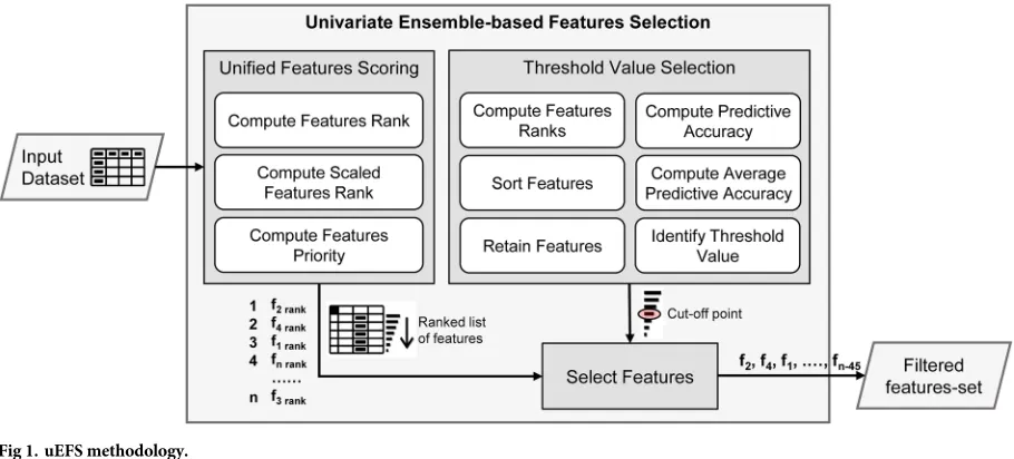
![Fig 2. UFS algorithm [19].](https://thumb-us.123doks.com/thumbv2/123dok_us/8393254.323992/8.612.119.577.78.250/fig-ufs-algorithm.webp)