Development of carbon based atomic oxygen sensors

(1)

University of Southampton Research Repository

ePrints Soton

Copyright © and Moral Rights for this thesis are retained by the author and/or other

copyright owners. A copy can be downloaded for personal non-commercial

research or study, without prior permission or charge. This thesis cannot be

reproduced or quoted extensively from without first obtaining permission in writing

from the copyright holder/s. The content must not be changed in any way or sold

commercially in any format or medium without the formal permission of the

copyright holders.

When referring to this work, full bibliographic details including the author, title,

awarding institution and date of the thesis must be given e.g.

AUTHOR (year of submission) "Full thesis title", University of Southampton, name

of the University School or Department, PhD Thesis, pagination

(2)

UNIVERSITY OF SOUTHAMPTON

FACULTY OF ENGINEERING, SCIENCE & MATHEMATICS

School of Engineering Sciences

Development of Carbon-Based Atomic Oxygen Sensors

by

Carl Barry White

Thesis for the degree of Doctor of Philosophy

(3)

UNIVERSITY OF SOUTHAMPTON ABSTRACT

FACULTY OF ENGINEERING, SCIENCE & MATHEMATICS SCHOOL OF ENGINEERING SCIENCES

Doctor of Philosophy

DEVELOPMENT OF CARBON-BASED ATOMIC OXYGEN SENSORS by Carl Barry White

This work focuses on the development of a hyperthermal, neutral atomic oxygen (AO) sensor that can be used on a wide variety of spacecraft platforms and in ground-based atomic oxygen environment simulators. Carbon has been identified as the sensitive medium for sensing the AO and one of the most important aspects of this work was selecting the most appropriate type of carbon for a particular AO dose.

This work fabricates carbon films by physical vapour deposition (PVD) and screen-printing techniques to provide different thicknesses and erosion rates, which affect the sensitivity and life of the sensor. Screen-printed films provided a useful means of detecting large AO doses (fluences), whilst the thinner PVD films provide a more sensitive film for smaller AO fluences. Attempts are also made at interpreting the data to measure the rate of AO (flux).

A combination of characterisation techniques confirm that the carbon films react by chemical removal of the carbon, which is also detected by measuring changes in electrical resistance. This work also postulates that the disorder of the carbon films (measured by Raman spectroscopy) can have an effect on the erosion rate of the material.

Results from this work will eventually be compared with two low Earth orbiting spacecraft experiments: STORM on the International Space Station and CANX-2. These experiments are described and engineering details relevant to the sensors are also included.

(4)

LIST OF FIGURES

Figure 1: Compositional variation of the thermosphere ... 9

Figure 2: Variation of AO abundance within the thermosphere ... 10

Figure 3: Solar illuminated shuttle tail-fin (left) and shuttle glow during eclipse (right). Image courtesy of NASA... 15

Figure 4: SEM image of particle on Kapton exposed to ~1.4x1020 atoms/cm-2, x5000 taken from [53]... 16

Figure 5: Silver film resistance-thickness variation [10] ... 27

Figure 6: Ideal ZnO actinometer characteristics [15] ... 31

Figure 7: Actual ZnO actinometer response to AO [93]... 32

Figure 8: Actual ZnO actinometer regeneration performance [15] ... 32

Figure 9: Variation of resistivity as a function of thickness ... 36

Figure 10: Schematic of yttria-stabilised zirconia (YSZ) actinometer [9]... 41

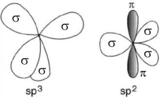
Figure 11: Schematic of sp3 and sp2 hybridised carbon atoms. ... 46

Figure 12: Diamond and graphite atomic arrangement... 48

Figure 13: Amorphous carbon ternary phase diagram from [108] ... 50

Figure 14: Measurements from a QCM coated with two different carbon films and exposed to an AO environment [103] ... 58

Figure 15: Flux dependent erosion yield of an amorphous carbon film, data plotted from [138] ... 62

Figure 16: Temperature dependent erosion yield of microcrystalline carbon [99].... 63

Figure 17: Beam energy dependent erosion yield of microcrystalline carbon [99] ... 64

Figure 18: MEDET on EuTEF [29] ... 69

Figure 19: The STORM module ... 70

Figure 20: Carbon actinometers on ram face PCB... 70

Figure 21: Computer generated model of the CANX-2 nanosatellite [21]... 73

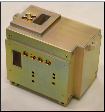
Figure 22: CANX-2 AO experiment module... 74

Figure 23: Two point contact layout ... 77

Figure 24: Interdigitated array layout ... 77

Figure 25: Screen printed heater layout ... 78

Figure 26: Coupon and sensor designation ... 79

(11)

Figure 28: Electron beam evaporation facility... 82

Figure 29: Screen printing technique ... 83

Figure 30: Schematic of ATOX facility... 87

Figure 31: Samples in ATOX before closure and pump down... 89

Figure 32: ATOX facility flux decay over ES1 ... 92

Figure 33: Sensor masking regime of coupon 02-01 for each AO exposure ... 93

Figure 34: IT/IG variation with sp3 content[27]... 101

Figure 35: D-peak breathing mode ... 102

Figure 36: Variation of the D and G-peaks with excitation energy[161] ... 102

Figure 37: ID/IG variation with in-plane correlation length, La [105]. ... 103

Figure 38: The Renishaw inVia Raman spectrometer ... 105

Figure 39: Raman spectrum of polycrystalline diamond reference ... 106

Figure 40: Raman spectrum of HOPG reference ... 107

Figure 41: Alumina Raman spectrum ... 108

Figure 42: Evaporated film exposure (versus fluence) ... 112

Figure 43: Evaporated film exposure (runs 1 and 2) ... 112

Figure 44: Evaporated sensor responses to UV and AO+UV (run 5)... 113

Figure 45: Evaporated sensor ANLE (run 5) ... 114

Figure 46: Evaporated sensor exposures (run 4)... 115

Figure 47: Evaporated sensor response to AO (Run 6a)... 116

Figure 48: Evaporated sensor ANLE (run 6a) ... 116

Figure 49: FEGSEM image of unexposed evaporated sensor ... 117

Figure 50: FEGSEM image of AO exposed evaporated sensor... 117

Figure 51: SEM image of remaining evaporated carbon exposed to AO ... 118

Figure 52: Unexposed evaporated sensor (run 6) ... 119

Figure 53: Exposed evaporated sensor (run 6)... 119

Figure 54: Curve fit of Raman spectrum for annealed evaporated film (coupon 26) ... 121

Figure 55: Raman spectra of evaporated film (coupon 202), covered film spectra are dashed... 121

Figure 56: Raman spectra of untreated evaporated films, exposed spectra is dashed ... 122

(12)

Figure 58: Curve fit of Raman spectrum for DS2 evaporated film... 123

Figure 59: Raman spectrum of coupon 26 with 510nm excitation wavelength... 124

Figure 60: Sputtered film exposure (run 1)... 129

Figure 61: Sputtered film exposure (run 1) versus fluence... 130

Figure 62: Sputtered sensor exposure (run 5) ... 131

Figure 63: Sputtered sensor ANLE (run 5) ... 131

Figure 64: SEM image of sputtered film annealed to 600°C for 100 minutes... 132

Figure 65: SEM image of sputtered film annealed to 600°C for 200 minutes... 133

Figure 66: Unexposed sputtered sensor ... 133

Figure 67: Exposed sputtered sensor ... 134

Figure 68: Sputtered sensor topography after AO exposure (run 5)... 134

Figure 69: Raman spectra of coupons 21 and 23 (dashed) before exposure to AO. 136 Figure 70: Curve fit of Raman spectrum for DS1sputtered film ... 137

Figure 71: Raman spectra of coupon 21 films before and after (dashed) AO exposure ... 138

Figure 72: Raman spectra of sputtered film (coupon 23) before and after AO exposure ... 138

Figure 73: Interdigitated sensor comparison (AO exposed is dashed) ... 139

Figure 74: Curve fit of Raman spectrum from coupon 102. ... 140

Figure 75: Curve fit of coupon 104 Raman spectrum... 140

Figure 76: Erosion yield variation with sp3 content... 144

Figure 77: Screen-printed film exposure (run 1)... 147

Figure 78: Screen-printed film exposure as a function of fluence (run 1) ... 148

Figure 79: Thick film exposure (run 2)... 148

Figure 80: Thick film sensor ANLE with respect to fitted lines (run 2)... 150

Figure 81: Run 3 gradient changes ... 151

Figure 82: Screen-printed films exposed to a plasma asher [189] ... 152

Figure 83: Unexposed thick film sensor ... 153

Figure 84: Exposed thick film sensor... 153

Figure 85: Raman spectra of unexposed thick film (coupon 2) ... 155

Figure 86: Raman spectra of unexposed screen-printed films ... 155

Figure 87: Raman spectra of exposed screen-printed films ... 156

(13)

Figure 89: Curve fit of CH stretching zone found on screen-printed UV spectra ... 157

Figure 90: Screen-printed film lower spectral range... 158

Figure 91: Response decay during run 6... 163

Figure 92: Comparison of silver and carbon actinometers ... 164

Figure 93: Lifetime-sensitivity map of exposed materials... 166

Figure 94: UV Raman G-position versus sp3 free evaporated film normalised erosion yield. Vector marked by arrows indicates potential error. ... 168

Figure 95: Curve fit of Raman spectrum for annealed evaporated film (coupon 26) ... 194

Figure 96: Curve fit of Raman spectrum for untreated evaporated film (coupon 41) ... 195

Figure 97: Curve fit of Raman spectrum for DS2 evaporated film... 197

Figure 98: Curve fit of Raman spectrum for DS1sputtered film ... 198

Figure 99: Variation of G-peak displacement for a-C1-x:Six:H alloys[26]... 200

Figure 100: Urethane Linkage ... 202

Figure 101: Screen-printed film lower spectral range... 203

(14)

LIST OF TABLES

Table 1: A sample of modern AO simulation methods... 13

Table 2: Common chemical bond strengths[52] ... 15

Table 3:Properties of silver and its oxides from [73] and [11] ... 23

Table 4: Summary of silver actinometer flights... 26

Table 5: Typical errors of commercial sensors ... 40

Table 6: Summary of actinometer material properties... 44

Table 7: The bonds of carbon ... 47

Table 8: Sample properties of some different kinds of carbon and carbon-based materials ... 50

Table 9: Summary of AO reaction with carbon ... 66

Table 10: Summary of AO reaction with carbon (continued)... 67

Table 11: STORM system characteristics... 69

Table 12: Fluence estimates for STORM based on figures from CEPF [22] ... 74

Table 13: Fluence estimates for CANX2 based on figures from CEPF ... 75

Table 14: CQCM specification ... 89

Table 15: Atomic oxygen exposure data... 91

Table 16: Temperature settings for first exposure session... 91

Table 17: Raman peak assignments for carbon... 100

Table 18: Order of characterisation beam energies... 109

Table 19: Summary of evaporated depositions... 110

Table 20: Summary of evaporated film erosion yields ... 111

Table 21: Evaporated film content (at. %) ... 120

Table 22: Hydrogen content estimates... 124

Table 23: Peak fits of coupon 202 ... 126

Table 24: Summary of sputtered depositions... 127

Table 25: Comparison of theoretical and measured erosion yields ... 128

Table 26: Sputtered film content (Atomic percent) ... 135

Table 27: DS2 Sputtered film content (Atomic percent) ... 135

Table 28: Hydrogen content estimations... 136

Table 29: Spectral change with AO dose for DS1 sputtered sensor ... 139

(15)

Table 31: Screen printed depositions ... 145

Table 32: Measured and estimated erosion yields of screen-printed films († treated as a fresh sensor) ... 146

Table 33: Screen printed film content (atomic percent)... 154

Table 34: Hydrogen content estimates... 159

Table 35: Specific gravities of possible film constituents ... 160

Table 36: IT/IG ratios for DS1 as deposited evaporated sensors... 196

Table 37: Raman characteristic frequencies of potential oxygen bonding regimes. 199 Table 38: Raman spectra details ... 204

(16)

AUTHORS DECLARATION

I, Carl White declare that this report entitled Development of Carbon-Based Atomic

Oxygen Sensors and the work presented in it, are my own.

I confirm that:

• This work was done wholly or mainly while in the candidature for a research

degree at this University;

• Where any part of this thesis has previously been submitted for a degree or

any other qualification at this university or any other institution, this has clearly been stated;

• Where I have consulted the published work of others, this is always clearly

attributed;

• Where I have quoted from the work of others, the source is always given.

With the such quotations, this thesis is entirely my own work;

• I have acknowledged all main sources of help;

• Where the thesis is based on work done by myself jointly with others, I have

made clear exactly what was done by others and what I have contributed myself.

Name:

Signature:

(17)

ACRONYMS

a-C Amorphous Carbon

a-C: H Hydrogenated Amorphous Carbon

a-C: Si: H Hydrogenated Amorphous Carbon-Silicon alloy

ADC Analogue to Digital Converter

ANLE Actinometer Non-Linearity Error

AO Atomic Oxygen

AOE Atomic Oxygen Experiment

ATOX ATomic OXygen test rig (hyperthermal source)

BREMSAT University of BREMen SATellite

CANX Canadian Advanced Nanospace Experiment

CCD Charge-Coupled Device

CHDI trans-CycloHexane DiIsocyanate

CONCAP CONsortium for materials development in space Complex Autonomous Payload

CNES Centre National D’Etudes Spatiales

C-QCM Carbon-coated QCM

CVD Chemical Vapour Deposition

DC Direct Current

DLC Diamond-Like Carbon

DMM Digital Multimeter

DS Deposition Session

E-Beam Electron Beam

EDS Energy Dispersive x-ray Spectroscopy

EDX Energy Dispersive X-ray spectroscopy

ESA European Space Agency

ESTEC European Space research and Technology Centre

EUTEF European Technology Exposure Facility

EUV Extreme Ultraviolet

FEGSEM Field Emission Gun Scanning Electron Microscope

FIPEX Flux Probe EXperiment

(18)

GPS Global Positioning System

GTO Geostationary Transfer Orbit

HOPG Highly Orientated Pyrolytic Graphite

HPIB Hewlett-Packard Instrument Bus

IPA IsoPropyl Alcohol

IR Infrared

IRDT Inflatable Re-entry and Descent Technology ISAC International Solar Array Coupon

ISS International Space Station

ITL Integrity Testing Laboratories

KWS Kapton Witness Sample

LANL Los Alamos National Laboratory

LDCE Limited Duration space environment Candidate materials Exposure payload

LDEF Long Duration Exposure Facility

LED Light Emitting Diode

LEO Low Earth Orbit

MACOR Machinable glass ceramic

MEDET Materials Exposure and Degradation Experiment on EuTEF

MEMS Micro Electro-Mechanical System

MSERD Mono-Substituted Epoxide Ring Deformation

NASA National Aeronautics and Space Administration

ONERA Office National d’Etudes et de Recherches Aerospatiales

PA Polyacetylene

PC Personal Computer

PCB Printed Circuit Board

PL PhotoLuminescence

PPDI Para-Phenylene DiIsocyanate

PSU Pennsylvania State University

PTF Polymer Thick Film

PTFE PolyTetraFluoroEthylene

PU Polyurethane

PVD Physical Vapour Deposition

(19)

RF Radio Frequency

SAA South Atlantic Anomaly

SAE Systematic Actinometer Error

SCD Semi-Conducting Detector

SEM Scanning Electron Microscope

SESAM Surface Effects SAmple Monitor

SiC Silicon Carbide

SIMS School of Industrial and Manufacturing Science (Cranfield University)

STORM Southampton Transient Oxygen and Radiation Monitor

STRV Space Technology Research Vehicle

STM Scanning Tunnelling Microscopy

STS Space Transportation System (the Space Shuttle)

SXR Soft X-Ray

ta-C Tetrahedral Amorphous Carbon

ta-C:H Hydrogenated Tetrahedral Amorphous Carbon

TEA Transversely Excited Atmospheric

TEAMSAT Technology, science and Education experiments Added to MaqSAT

TEXUS Unknown, sounding rocket missions

TEY Theoretical Erosion Yield

TQCM Temperature controlled QCM

UTIAS University of Toronto Institute of Aerospace Studies

UV UltraViolet

VUV Vacuum UltraViolet

XPS X-ray Photoelectron Spectroscopy

YSZ Yttria-Stabilised Zirconia

(20)

ACKNOWLEDGMENTS

Firstly, I think it is best to thank my supervisors Graham Roberts and Alan Chambers for

providing the exciting opportunities, financial wizardry, their valuable time…and patience.

The Engineering and Physical Sciences Research Council, World Universities Network and

the Royal Academy of Engineering should also be noted for their invaluable financial

contributions.

This PhD would have not have been possible without the help of the following people:

• Marc van Eesbeek, Adrian Tighe and the others at ESTEC who offered their time,

hospitality and use of the ATOX facility.

• John Badding, Bryan Jackson and Neil Baril of PSU who provided the facilities and

substantial expertise for Raman spectroscopy.

• Ken Lawson and Jeff Rao of Cranfield University SIMS, who deposited the carbon

films and provided tasty pizzas every time I visited.

• John Atkinson and Zhige (Gary) Zhang of the Thick Film Unit, who were once again

invaluable to the fabrication of the sensor substrates.

• Jacob Kleiman and Zelina Iskanderova of ITL Inc for their plasma asher work.

• Duncan Goulty for all the hard work designing, building, testing and integrating the

Southampton Transient Oxygen and Radiation Monitor with the MEDET module.

During the course of my research I have spent substantial periods on my own; either in my

office or in far away lands. So thanks to Martijn, Dave, Paolo (the ‘Bulk’), Christoph,

Thomas, Ian W and the others for the office distractions and to Steven, Ian H, Jürgen and

Stuart for when the office just got too quiet. I should also note the conversations with Juan

Carlos.

(21)

1 INTRODUCTION

1.1 The Spacecraft Environment

Regardless of the mission, spacecraft operate in harsh environments. Perhaps the most influential body to the spacecraft environment is the sun, which (excluding planetary decay processes) provides 99.9% of the energy in the solar system[1]. Energy is emitted across the whole electromagnetic spectrum, but particularly in the form of infra-red (IR), visible, ultra violet (UV) and X-rays. The sun not only emits massive amounts of energy but also matter, predominantly in the form of electrons and protons. This stream of matter from the sun is called the solar wind.

Van Allen radiation belts contain energetic protons and electrons from the solar wind that are trapped inside the Earth’s magnetic field. These trapped particles are known to degrade electronic parts due to high-energy particle impact, affecting both the

energy structure and lattice structure of semiconductors [2]. Normally, low Earth orbits (those below 1000km) are too low for the Van Allen belt to cause concern, however asymmetry in the Earth’s magnetic field reduces the altitude of this belt above the South Atlantic Ocean in a region called the South Atlantic Anomaly (SAA), which can at times be troublesome [3].

(22)

The orbit of a satellite alone can greatly influence its environment, particularly with respect to temperature. The thermal environment of a spacecraft is influenced predominantly by direct heating from the Sun. As a low Earth orbit (LEO) satellite enters or exits the Earth’s shadow, very high heating or cooling rates can occur that can warp or fatigue materials to the point of failure [5].

Last but by no means least, it is important to describe the contributions made by Earth’s atmosphere. In the upper atmosphere, vacuum (10-200nm) and extreme (1-30nm) ultra-violet light (VUV and EUV) from the Sun interact with atmospheric

species to create the ionosphere, an atmospheric layer of heated plasma. Orbiting spacecraft passing through the ionosphere may suffer rapid electrical discharges that can damage instrumentation and material surfaces should charging effects not be accounted for in the spacecraft design [6].

Solar energy also affects the density of the thermosphere, a region of Earth’s atmosphere between 90–600 kilometres altitude. Although the density of the thermosphere is low, the drag forces present greatly affect the orbits and trajectories of passing spacecraft due to the relative speed of impact with atmospheric species. Drag should be countered by an appropriate propulsion system to prevent re-entry into the Earth’s lower atmosphere and the obvious loss of the spacecraft [7]. More importantly for this thesis, important chemical processes are occurring as a

spacecraft impacts the thermosphere. The most abundant species in the thermosphere is atomic oxygen (AO).

AO is formed by the UV dissociation of molecular oxygen and is therefore a process driven by solar emissions. As AO strikes forward (ram) facing spacecraft surfaces at high relative velocities, several important phenomena occur. One of the effects is to degrade these surfaces, often by erosion.

The modification of surfaces by AO is an extremely important consideration for spacecraft developers. Modified surfaces can lead to changes in thermo-optical

(23)

1.2 Atomic Oxygen Detection

To aid spacecraft designers select and develop appropriate materials to be exposed to an AO environment, it is important to assess the concentration or typical doses of the species in a particular orbital regime, or a man-made simulator.

The University of Southampton has developed sensors that are suitable for measuring the concentration of atomic oxygen at different Earth orbits[9]. In the past, the

university has developed silver sensors (or actinometers) that measure AO flux by monitoring changes in electrical resistance across an eroding silver film [10-12]. Unfortunately, the effectiveness of these sensors is restricted by the development of an oxide film as the silver reacts with AO, making sensor response dependent on a diffusion-based mechanism. These silver actinometers also have a limited life, as eventually the film will react completely.

More recently, the university has been developing semi-conducting films, made from n-type zinc oxide (ZnO), for the purposes of AO detection [13-15]. These sensors do

not erode, but exhibit a change in resistance as the zinc oxide adsorbs AO. When heated, the zinc oxide expels the adsorbed AO, restoring the resistance to

approximately the ‘pre-exposure’ values. This so-called ‘regeneration’ gives a much-extended sensor lifetime, over the silver actinometers.

Despite the advantages of the zinc oxide sensor there remain some difficulties. The zinc oxide sensors have a complex response to AO exposure, and suffer electrically conductive hysteresis effects when regenerated. Whilst some of these difficulties may be overcome by suitable development, these sensors are inherently unsuitable for continuous material characterisation purposes, as AO measurement is interrupted as the sensor is regenerated [9].

(24)

The response from carbon sensors is known to be much simpler than ZnO sensors, so offering an advantage.

An interesting aspect of carbon is that it is commonly available in two different allotropes and many other different forms, as will be highlighted in a later chapter. The many possible variants could mean that a wide range of different responses to AO are also available, which have not yet been researched. This work will focus on developing suitable carbon materials for AO sensing in a wide range of orbital applications.

1.3 Spaceflight Opportunity

During the course of the research presented here, there have been two flight opportunities to test the carbon materials.

A package, named the European Technology Exposure Facility (EuTEF), is due to fly aboard the International Space Station (ISS), a manned low Earth orbiting

experimental platform. EuTEF will contain a variety of experimental platforms that are directly exposed to the LEO environment for a period of 3 years. The Materials Exposure and Degradation Experiment on EuTEF (MEDET) is one such experiment [16].

MEDET is a project run jointly between the European Space Agency (ESA), Centre National d’Etudes Spatiales (CNES), Office National d’Etudes et de Recherches Aerospatiales (ONERA) and the University of Southampton. MEDET will be used primarily to monitor the effects of the LEO environment (such as solar energy emission, space debris and AO fluxes) on a selection of materials.

The Southampton Transient Oxygen and Radiation Monitor (STORM) aboard MEDET will be used to monitor X-ray, UV and AO fluxes and will house the developed AO sensor [17].

(25)

operated at significantly less cost than more traditional platforms. The advantage of actinometers over other existing AO sensing techniques is that they are very simple, lightweight and use only very small amounts of power, so they lend themselves well to such an application [9].

An opportunity to fly aboard a nano-satellite has also arisen during the course of this work. The Canadian Advanced Nanospace Experiment (CANX) program is an initiative set up by the University of Toronto Institute for Aerospace Studies Space Flight Laboratory (UTIAS/SFL) [21]. The second experiment of the program,

CANX-2 is a 3.5kg nanosatellite used as a test-bed for future formation flying missions. The experimental package consists of an atmospheric spectrometer, a dual band GPS receiver/antenna and an atomic oxygen degradation experiment.

The orbital parameters for this nano-satellite are much less defined than the ISS mission. In order to save launch costs, the satellite orbit is defined by the

requirements of a larger satellite to which the nano-satellite is ‘piggy-backed’ or simply by the chosen launch vehicle capabilities. The CANX-2 mission is designed to orbit Earth for a period of 1 year before undertaking a de-orbit manoeuvre. The type of orbit and altitude were not defined during satellite constuction, but was later set for a 600km LEO. This will naturally impact the AO dose and the thermal environment of the spacecraft.

(26)

1.4 Project Aims

The aims of this project are:

• To investigate the nature of the carbon/AO interaction including reaction

characteristics and rates, with a wide variety of carbon materials.

• To analyse the data acquired from carbon-based sensors and how it relates to

AO dose.

• To develop carbon-based films suitable for a variety of atomic oxygen

sensing missions, including the long duration MEDET mission and the shorter duration CANX2 mission.

1.5 Manuscript Layout

This document begins with a literature review of AO, its simulation and

measurement. The literature review then continues, covering actinometer research to date before describing carbon and its various reactions with AO.

The experimental phase of this work is then described. Chapter 5 describes the general design of the actinometer devices used in this work and their integration with the ISS and CANX2.

Chapters 6 and 7 provide details of the experimental design, AO simulation

facilities and characterisation methods. Chapter 7 also gives some detail on the latest

research into interpretation of Raman spectra, as the understanding of this technique has improved significantly in recent years [23-27].

(27)

chapter. Chapter 8 covers the evaporated films, Chapter 9 the sputtered and Chapter 10 the screen-printed film results.

In Chapter 11 each deposition method is compared in terms of the reactions with AO and the use of each film as a sensing material. The work is concluded and suggestions for further work are made in Chapter 12.

1.6 Publications

(28)

2 THERMOSPHERIC ATOMIC OXYGEN, ITS SIMULATION AND

MEASUREMENT

2.1 Introduction

This chapter will be used to summarise the processes by which atomic oxygen is formed, both by natural and man made processes. This chapter will then go on to summarise the effects of atomic oxygen and the techniques used to measure it. It should be noted that these topics are very comprehensive subjects that could each demand a stand-alone chapter. However, Harris [35] and Osborne [15] have reviewed this work extensively, so without repeating these works, each topic is summarised and reviewed in a single chapter for completeness.

2.2 Atomic Oxygen Formation

Atomic oxygen is commonly formed by the dissociation of molecular oxygen. Dissociation occurs when sufficient energy is provided to the oxygen molecule, where the sources of energy can vary greatly.

2.2.1 Atmospheric AO formation

Five distinct layers based on thermal characteristics, chemical composition, movement and density identify the Earth’s neutral atmosphere. These layers are called the troposphere (0-15km above Earth’s surface), stratosphere (15-50km), mesosphere (50-85km), the thermosphere (85-600km), where most low Earth orbits take place and the exosphere (>600km) [36].

(29)

By a process of convection and diffusion, oxygen is found in the stratosphere. At these altitudes atmospheric density is much lower and UV solar energy becomes strong enough to split oxygen molecules into neutral atomic oxygen, a process called photo-dissociation. In the stratosphere, these oxygen atoms are free to recombine into a variety of molecules, the most important one of which is ozone (O3). The ozone

layer lies within the stratosphere [37].

At greater altitudes atmospheric species become excited as they absorb the Sun’s energy until the thermosphere is reached. Like the stratosphere, photo-dissociation of

molecular oxygen takes place within the thermosphere. Atomic oxygen (AO) is not the main constituent in the stratosphere because mean free paths allow sufficient particle collisions to form new molecules. However, the lower density of the thermosphere does not allow such collisions to take place and so neutral AO becomes the dominant species. In fact, as altitude increases the relative concentrations of AO continue to increase due to a reduction in recombination probability [8]. Figure 1 shows the typical compositional variation of the major atmospheric constituents over the altitude range 100 - 800 km.

100 200 300 400 500 600 700 800

Number density (cm-3)

A lt it u d e (k m ) _O N2 O2 He

[image:29.595.190.453.454.608.2]

105 106 107 108 109 1010 1011 1012 1013

Figure 1: Compositional variation of the thermosphere [15]

(30)

number density with solar activity is demonstrated in Figure 2, which shows curves for solar minimum, maximum and mean irradiation levels. Clearly, the effect of solar activity is most significant at the higher altitudes, where AO density may alter by as much as two orders of magnitude between solar minimum and maximum. Near the bottom of the thermosphere, in comparison, the density varies by much less than one order of magnitude.

100 200 300 400 500 600 700 800

Number density (cm-3)

A lt it u d e (k m ) Solar minimum Solar mean Solar maximum

104 105 106 107 108 109 1010 1011 1012

Figure 2: Variation of AO abundance within the thermosphere [15]

It should be noted that AO is free to move within the thermosphere, and between atmospheric layers. However, the speed of these species relative to an impacting spacecraft is sufficiently low to be considered zero. Although the atoms have nominally zero translational energy, they are at a temperature above zero Kelvin so have a thermal energy described by the following equation of an ideal monatomic gas: e T k eV Energy B 2 3 )

( = Equation 1

where

kB=Boltzmanns constant ( 1.38x10-23 J/atom/K), T = gas temperature (K) and

(31)

At typical LEO altitudes the mean thermospheric temperature is ~1000K, which

gives an AO thermal energy of ~0.14eV.

Spacecraft pass through the Earth’s atmosphere at very high velocities, LEO

spacecraft travel at approximately 8 km/s [38] and some elliptical orbits like that of

geo-stationary transfer orbits (GTO) can reach speeds of 11km/s or more at perigee

[11]. The oxygen atoms have some thermal energy, but this is usually neglected

because of the high relative speeds between the atoms and the spacecraft. The high

velocities give the atoms a high translational or kinetic energy, as defined by the

equation below.

e v m eV

Energy o s c

2 ) (

2 / 1

= Equation 2

where

mo1=O atom mass, vs/c=spacecraft velocity, e=electron charge (1.6x10-19C).

2.2.2 Ground-based, man-made AO

Spaceflight experiments are inherently expensive and can sometimes be

impractical to assess AO effects on materials. For fundamental AO research such as

the:

1) determination and prediction of erosion yields,

2) calibration of sensors and

3) investigation of synergistic effects,

AO induced effects need to be separated from other parameters such as UV and

micrometeoroid degradation at lower costs than spacecraft experiments.

(32)

simulation facilities [39]. The fundamental difference between the formation of

atmospheric AO and that simulated on the ground is that ground based sources may

need to adopt a method of accelerating AO to speeds comparable to that of impacting

spacecraft. When accelerating AO additional energy, surplus to dissociation, is

required. A risk with providing this additional energy is that some energy will be

used to strip off electrons and form oxygen ions rather than fast neutral AO. This

statement somewhat summarises why there are a variety of AO sources with

different beam energies and ion/neutral species content. Another factor that

complicates AO simulation is that in some cases testing needs to be accelerated.

Accelerated tests require yet more energy to dissociate greater concentrations of

molecular oxygen, and so care must be taken to ensure that energy is distributed

equally to each molecule, otherwise beam content could be somewhat more variable.

Table 1 lists some of the various methods by which atomic oxygen is created.

Perhaps the most curious omission from the table is that UV photo-dissociation is not

currently used to break-down molecular oxygen, as evident in the LEO environment.

There is no documentation found explaining why this is so. Also included are two

methods that produce predominantly oxygen ions and are commonly used in the AO

community. Whilst these sources do not strictly produce neutral AO, they provide a

simple means to accelerate oxygen erosion, when it is not possible to use existing

(33)

AO Formation Method Beam Acceleration/ Delivery Mode Beam Energy (eV) Flux (species/

cm2 /s)

Flux Composition

(%)

Reference

RF Plasma Electrostatic Pulsed 5 5x1015 (1/99) O

+ /O (+VUV) [41, 42] Pulsed Laser Breakdown

of O2

Detonation Wave in Supersonic

Nozzle

Pulsed 1-16 1015-1017 (10/90) O2 /O

(+VUV) [43, 44]

Pulsed Laser Breakdown

of O2

Detonation Wave in Supersonic

Nozzle

Pulsed 5 1014 (60/40) O2 /O [39]

Laser Breakdown of O2 in Ar

Supersonic

Expansion Continuous 1-3 1016 (90/7/3) Ar/ O2 /O

[38, 45] Microwave

Breakdown of O2 in He

Supersonic

Expansion Continuous 1-3 1017 (97/1/2) He/ O2 /O

[46] Arc

discharge Electrostatic Continuous 30-50 1014 ~(100) O+ [39] O2 dissociation/ diffusion through Ag foil Electron-stimulated desorption

Continuous 5 5x1013 ~(100) O [47]

Table 1: A sample of modern AO simulation methods

2.3 AO effects

The most significant effects of AO on a spacecraft are drag, shuttle glow and

(34)

2.3.1 Drag

As a spacecraft passes through the Earth’s atmosphere there will be a reaction

force from the oxygen atoms that will collectively slow the spacecraft. Drag is an

important problem because as a spacecraft slows down, it will gradually de-orbit.

The Long Duration Exposure Facility (LDEF) is an example of how drag can affect

the performance of a satellite. Launched in 1984 by the Challenger Space Shuttle, the

LDEF was an orbital platform that exposed a wide range of candidate spacecraft

materials to the LEO environment for a period of 2114 days [48]. During the course

of its mission, LDEF had slowed to such an extent that its retrieval date was brought

forward to prevent a dangerous de-orbit [49]. Although AO does contribute to drag

forces, so do a number of other effects such as micrometeoroid impacts that are

beyond the scope of this work.

2.3.2 Shuttle glow

Shuttle glow is a phenomenon where atomic oxygen atoms interact with

nitrogen-based species around a spacecraft, creating an optical emission [50]. Nitrogen atoms,

molecules and nitrous oxide molecules that are present in the thermosphere, the

spacecraft materials or mass ejections (like reaction thruster firings) can be found on

or surrounding spacecraft surfaces and in the wake of the vehicle. The AO reacts to

form vibrationally excited species, which then relax to the ground state by photon

emission, thereby producing an optical emission, or glow (Figure 3). The glow has

emissions in the infra-red, visible and UV wavelengths and can interfere with the

operation of optical devices, especially those operating in these spectral bands [50].

Shuttle glow is so termed because its presence was first confirmed by optical

(35)

[image:35.595.255.384.443.609.2]

Figure 3: Solar illuminated shuttle tail-fin (left) and shuttle glow during eclipse (right). Image courtesy of NASA.

2.3.3 Surface modification

As a spacecraft collides with high-energy AO atoms, susceptible materials on the

forward facing (ram) surfaces can react with the oxygen if there is sufficient energy

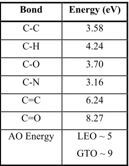
to break the chemical bonds. Table 2 shows some important bonds and their

associated energies found in a variety of spacecraft polymers. The chemical reactions

that can take place have different effects on different materials. The oxides that form

during these reactions can be classed into two kinds: gaseous (volatile) or solid

(stable).

Bond Energy (eV)

C-C 3.58

C-H 4.24

C-O 3.70

C-N 3.16

C=C 6.24

C=O 8.27

AO Energy LEO ~ 5 GTO ~ 9

Table 2: Common chemical bond strengths[52]

Gaseous oxides are often found in the reaction with polymers and usually leave the

surface of the parent material, causing it to recede. Typical oxides are CO, CO2 and

NO2. Figure 4 shows a scanning electron microscope (SEM) image of a Kapton-H

polymer post AO exposure. Kapton-H is a common spacecraft material used on

(36)

particle inadvertently left on the surface has protected the underlying material from

AO attack. It can be seen that the material exposed to AO has eroded somewhat,

leaving a rough grass, or rug-like texture. The texturing seen here is typical for many

kinds of carbon-based materials.

Figure 4: SEM image of particle on Kapton exposed to

~1.4x1020 atoms/cm-2, x5000 taken from [53]

AO may also react with certain materials to form a solid oxide, causing the mass of

the sample to increase. Solid oxides may be porous to AO and other species, as in the

case of silver oxides or form a protective barrier, as with aluminium.

Irrespective of the type of oxide, the standard method of defining reaction rates of

virgin material is the erosion yield, as defined by equation 3 [48].

F FA

m

Y

τ

ρ

∆ = ∆

= Equation 3

Y=yield (cm3/atom),

∆

m =mass loss of virgin material (g), A=affected area (cm2),

ρ

=density (g/cm3),

∆τ

= thickness loss (cm) and F=AO fluence (atoms/cm2)

Another way of expressing reaction rate, but not as commonly used is the reaction

(37)

f y

P= Equation 4

where y = rate of material loss (atoms/cm2/s), f = AO flux (atoms/cm2/s).

In some cases, UV illuminating on material surfaces is known to enhance the erosive

effect of AO. This effect, termed ‘AO-UV synergism’, has undergone many studies

on various materials [55, 56]. Under certain conditions, one study has shown that the

erosion rate increases by up to 400% over non-illuminated Kapton samples [57].

2.4 AO measurement

There are a wide variety of AO sensing techniques as reviewed by Osborne et al

[9], which are described under the headings of 1) witness samples, 2) mass

spectrometry, 3) catalytic probes, 4) optical methods, 5) crystal microbalances, or 6)

actinometers. A brief summary of each method is provided in this section.

2.4.1 Witness Samples

Presently the accepted reference standard for AO measurement is by Kapton

witness sample (KWS) erosion [58, 59]. Witness samples are the simplest form of

AO measurement. Samples of material with a known erosion yield, which in the case

of Kapton is assumed to be 3x10-24cm3/atom, are exposed to the AO fluence. During

exposure the surface erodes, causing a change in surface profile and mass; measuring

these changes and using the data with equation 3 provide a fluence estimate.

The main advantages of this method are that it is small, light and does not require

power. This method is also very low cost provided mass and profile measurement

facilities are available. The simplicity of this method means that it can be applied to

any AO simulation facility and it is for this reason that it is useful as a common

(38)

The inherent problems with this method are that:

1. It is susceptible to contamination errors,

2. It does not provide in-situ measurements (it only provides post exposure

measurement of fluence)

3. The erosion yield of Kapton is very variable and

4. Accuracy is generally poor for low fluences.

The most significant disadvantage of this method is that the erosion yield of

Kapton is not always 3 x10-24cm3/atom. This value was derived from the early LEO

space shuttle missions [60], but subsequent ground based testing has revealed that the

erosion rate is proportional to beam energy, sample temperature and the relative

intensity of UV light and AO [57, 61]. In the latter case, for extremely high

intensities of UV (albeit unrealistic) the erosion rate is increased by 400%.

2.4.2 Mass Spectrometers

Contrasting greatly with witness sample measurement, mass spectrometers are one

of the most frequently used and sophisticated instruments for thermospheric

investigations. The main benefits of mass spectrometers are that they are able to

provide direct, time resolved measurements of thermospheric densities. They can

also make measurements of other neutral and charged species [62]. Disadvantages

include mass, power and cost budgets. With the ever-increasing use of small satellite

technology, this approach to AO measurement may be used less frequently. The

sophisticated nature of this technique also means it would be difficult to use as a

measurement standard for ground based applications, as different AO facilities would

require different systems.

2.4.3 Catalytic Probes

(39)

reaction on a catalytic surface [63]. Thermocouples attached to the surface of the

catalyst are used to measure the heat energy released during recombination. The

amount of heat released, and hence the temperature, is proportional to the amount of

AO impinging the surface. These sensors are simple, low mass, low size and low

power instruments, but are only useful in steady thermal conditions, and so are

generally unsuited for orbital applications and many ground based AO facilities

where temperatures are known to vary significantly.

2.4.4 Optical Methods

Optical methods are based on the measurement of the emission, scattering or

absorption of visible, infrared or ultraviolet radiation caused by atomic oxygen.

Optical methods vary significantly, but in general they are more complex systems

that consume more power and mass than many of the methods discussed above.

However, there are two recent exceptions to this general rule.

The first of these optical techniques measures the AO induced reflectance changes

of an optically thin metal film deposited on the end of an optical fibre [64-66]. As the

film is oxidised by AO, the reflectance of the fibre-film interface alters, thus the

change of reflectance can be associated with the accumulated AO exposure.

Reflectance changes are measured by passing the radiation from a light emitting

diode (LED) along the fibre and comparing the intensity of the back reflection to that

of the LED output.

A technique using the change in transmission of a polymethylmethacrylate

(Perspex ®) optical fibre subject to AO attack has also been proposed for a

micro-satellite application [9]. AO erosion of the fibre alters its transmissivity, which is

measured by shining LED light along the fibre and comparing intensities before and

after transmission.

Neither of the two optical methods described have flown successfully in space, but

their simplicity, low mass and power mean that these methods are promising for the

(40)

techniques are that once the reacting film becomes fully consumed, no further

measurements can be made.

2.4.5 Quartz Crystal Microbalances

Quartz-crystal microbalances (QCM) consist of essentially a piezo-excited quartz

crystal coated with a material sample that reacts with AO. Depending on the kind of

oxides developed, the mass of the crystal will either increase or decrease giving a

measurable change in resonant frequency.

This method is able to provide high resolution, in-situ measurements and can

therefore measure both flux and fluence. The sensors themselves are light, compact

and consume relatively small amounts of power. The other advantages of QCMs are

that a wide variety of materials can be deposited onto the crystal and if no coating is

applied have the ability to measure contamination [67]. These advantages mean that

QCMs have been used for a wide variety of sensing applications, both in orbit and in

ground based testing applications [68-71].

The QCM has moving parts, resonating by the order of 106 Hz, so there can be

reliability issues for the sensor. The electronics used to measure these high

frequencies are also moderately complex; detrimentally affecting cost and reliability.

Unless two QCMs are used, one coated and one uncoated, one of the side effects of

measuring mass changes is that the sensor is unable to discriminate contaminants and

absorbed species from AO erosion, which could lead to underestimates in the AO

flux readings.

2.4.6 Actinometers

Actinometers are electrically conducting films that experience a change in ohmic

resistance when exposed to AO. Either erosion of the conducting film or oxygen

absorption/adsorption into the film brings about the change in resistance [9]. These

(41)

They can provide in-situ measurements of flux and fluence and require very simple

electronics to do so. This makes the actinometer ideal for small satellite applications

where such issues are vitally important [11, 12, 14].

As actinometers are exposed directly to the space environment, there is the

possibility that the AO sensitive element becomes coated to some degree by

contaminants. Obviously this will have an effect on sensor response if the

contaminant is not easily removed by AO, leading to an underestimate in AO

fluence. However, all the other sensing methods described here have this problem

except for mass spectrometers. Another common problem shared with many other

sensing methods is that the eroding actinometers have a limited lifetime, although

using thicker or less sensitive materials to AO attack can increase this.

Actinometers that use adsorption as the sensing mechanism have the advantage of

being reused upon heating, but this consequently increases the power consumption

and complexity of the device. Adsorption devices also require disruption of the AO

measurement when being heated for re-use.

2.4.7 Summary

The measurement techniques summarised here span a wide range of operating

parameters and each technique has different advantages and disadvantages. The ideal

system would utilise the least amount of mass and power, have an infinite lifetime,

be simple to activate and have the ability to monitor fluxes of AO and other species

to a high-resolution, without being effected by contamination. Unfortunately there is

no such system and so measurement techniques have to be selected by the constraints

of the mission. As will be reviewed in the next chapter, actinometers have been

applied to a wide range of space missions, from micro-satellite applications to space

shuttle missions, as they are simple, inexpensive and have low mass and power

budgets. Most importantly of all, the lifetime of the actinometer can be adjusted to

meet the needs of a particular mission by using films of different materials. This

thesis will now describe how different actinometer materials respond to the AO

(42)

3 A REVIEW OF ATOMIC OXYGEN ACTINOMETERS

3.1 Introduction

As highlighted in the previous section, actinometers are a highly versatile and

inexpensive solution to atomic oxygen measurement. They offer a number of

advantages over other sensing techniques, particularly for space flight experiments

with low mass and power budgets [72]. The AO sensitive material used for the

actinometer greatly affects its response and its method of operation.

Actinometers are available in essentially two different forms: those that have a

limited useable lifetime (non-renewable) and those that do not (renewable).

• Non-renewable actinometers usually depend on a degrading chemical

reaction of some sort to measure atomic oxygen flux. Typical examples are

carbon film actinometers and silver film actinometers. Although the reaction

mechanisms of these two materials are different, material degradation plays a

fundamental sensing role in both cases. As AO reacts with the material the

volume of electrically conducting material falls and in most cases cannot be

recovered.

• Renewable actinometers do not depend on a degradation mechanism to

measure AO flux. Instead the exposed sensor material will typically absorb or

adsorb the oxygen atoms in some way, creating a resistance change. The

“renewable” aspect occurs when these oxygen atoms can be desorbed later in

the sensors life to return the actinometer back to (ideally) its original

condition.

Almost all the work carried out on actinometers has been on three types of film

(43)

oxide is the only material researched that can provide renewable properties. Other

materials, like osmium can also be used as the sensing element, but for various

reasons have not been studied thoroughly. This section will provide a comprehensive

review of previous work undertaken to develop these sensors, with particular

emphasis on the AO sensitive material.

3.2 Silver Actinometers

Before discussing the use of silver as a non-renewable actinometer, it is appropriate

to begin with a description of how the material reacts with AO.

3.2.1 Reactions with AO

Silver reactions with AO are:

2Ag (s) + O (g) → Ag2O (s)

Ag (s) + O (g) → AgO (s)

Under AO exposure Ag2O is formed when an excess of silver exists and AgO is

formed with an excess of AO. Some properties of silver and its oxides are given in

Table 3:

Property Ag Ag2O AgO

Density, g cm-3 10.49 7.14 7.44

Molar volume, cm-3 10.25 16.25 16.6

Resistivity at 20°°°°C,

Ω Ω Ω

Ω.cm 1.587 x 10

-6

108 14

High temperatures

(@1 bar) Melts at 960.8°C

Reduces to silver ~250°C

Decomposes to Ag2O

at ~110°C Table 3:Properties of silver and its oxides from [73] and [11]

Investigations by Oakes [74] involving the in-situ measurement of film mass during

(44)

increase is linear. After this, the oxide layer becomes diffusion limiting; the reaction

rate begins to slow because the oxygen atoms are diffusing through the oxide layer

before arriving at the virgin material. Over time the diffusing oxygen atoms may

recombine to form molecular oxygen, which being less reactive contributes to a

reduction in the reaction rate of the material [72, 75]. Additionally as less and less

silver atoms are available for reaction so the probability of an oxygen atom reacting

reduces [74].

Oakes [74] found that during the diffusion-limiting period, silver reacts to form the

peroxide AgO preferentially to Ag2O at an AO flux equivalent to 1x1015atoms/ cm2/s

and a sample temperature of 20°C. Unfortunately, this work was not able to

comment on the reaction products during the initial linear phase of reaction. The

preceding work of Moore [76] states that this initial layer also consists of AgO, but

unfortunately the flux used to obtain this result is not clear from the paper.

The linear reaction rate has been reported by many authors as independent of temperature and sample thickness between 0°C and 85°C [74, 77, 78]. This offers

some advantage over materials that do have temperature dependence, as a

temperature sensor or temperature controlling device may not need to be

incorporated into the design of the AO sensor, thus giving any sensor package

greater mass and power economy.

At temperatures above 80°C, the reaction rate of silver increases to a point where, at 150°C, the erosion rate is six times greater[38]. At this temperature, the oxides

formed were found to be predominantly Ag2O rather than the AgO observed at room

temperature. Unfortunately no flux values are quoted for comparison with Oakes

[74].

The linear reaction rate has also been reported as independent of AO energy between

1 and 12eV [74, 77, 79] using ground based simulation techniques. This means that

sensors flying on very different orbits can be compared easily, for example data from

(45)

It is interesting to note from Table 3 that as the silver oxides are heated they can

reduce back to silver. For AO measurement, this is a useful characteristic, as it would

appear the silver could act as a renewable AO sensor by the application of

temperature. The works of [80] and [76] have identified and demonstrated this effect,

stating that oxidised films can be recycled many times and will assimilate as much

oxygen as the original film. Whilst this system of operation adds an additional power

requirement and complexity to the actinometer, the benefits of having a sensor with a

nominally infinite lifetime could out-weigh the disadvantages. Indeed, if a small

single crystal of silver were used, the additional power requirement may be very

small. The main practical limitation to this idea is the potential of oxide layer flaking,

as described below.

Table 3 shows that the molar volumes of the oxides are approximately 60% greater

than the original silver material. Consequently, as the oxide layer builds up, stresses

develop between the metal and oxide causing the oxide layer to flake away; a

phenomenon that has been observed by a variety of space flight experiments and

ground based simulations[81-83]. Flaking of the oxide layer means that virgin

material will continually be exposed to atomic oxygen and react, unlike the

protective oxides formed on other metals such as aluminium or copper. If flaking is

allowed to occur, it will provide a mass loss and silver films will be unsuited to the

renewable approach mentioned above, because after regeneration the film will be

different to its pre-exposure condition. However, if the sensor is heated before oxides

detach (within the 250 angstrom oxide thickness limit, mentioned above) then there

could be some potential for silver as a renewable sensor material. Unfortunately there

is little other research investigating this aspect of silver.

3.2.2 Silver Actinometer Performance

Silver is perhaps the most frequently used actinometer material to date because silver

is well suited for sounding rocket missions that pioneered the use of actinometers in

the early nineteen seventies[84, 85]. Sounding rockets are not orbital platforms and

as such have very little time to react with AO. Silver is well suited for this purpose

(46)

A number of flight experiments have used silver actinometers for AO measurement

as listed in Table 4.

Flight Film Thickness Reference

Sounding Rockets 380-570 angstroms 10-100 angstroms

[85] [73]

STS-4 2250 angstroms [86]

STS- 41 (ISAC) 1.1 micrometers [87]

STS- 46 (CONCAP-II) 220 angstroms [88, 89]

STRV-1a 1836-2839 angstroms [11]

STS80 & STS85 (SESAM) 100 nanometres [90] Table 4: Summary of silver actinometer flights

Upon AO exposure, the silver film initially erodes in a linear fashion until a point

where the response becomes parabolic with fluence due to the continued growth of

the oxide layer. This point occurs when thicknesses are between 250 and 350

angstroms. As the oxide layer thickens, the time for the oxygen atoms to reach the

conducting virgin substrate increases and so a time lag between AO flux and sensor

response is observed. This phenomenon is called coasting [72]. These trends are seen

by all the experiments referenced above.

It is pertinent to point out that because the useful (linear) life of the sensor always

occurs within the first few hundred angstroms, no matter how much thicker the films

are than this, AO measurement is limited by a maximum measurable fluence dictated

by these first few hundred angstroms. Assuming an erosion yield of 141x10

-25

cm3/atom [72] and a thickness of 350 angstroms, this maximum fluence can be

calculated as being 2.5x1016atoms/cm2.

An important aspect of silver actinometer calibration is the need to associate a

resistance value with a thickness value. The change of thickness can then be

associated to an AO fluence, assuming that erosion yield is constant. Therefore an

understanding of film electrical properties is essential. The work of Harris [10] has

reviewed this topic in great detail for thin silver films.

At any given temperature the resistivity of bulk silver, or any metallic conductor, is

(47)

mean free path of electrons, the movement of free electrons becomes impaired, so

reducing the effective mean free path and increasing resistivity.

The mean free path of silver is found experimentally and theoretically to lie within

the range of 500 to 530 angstroms[10, 91, 92]. Since the useful, linear life of silver

actinometers lies somewhere within the first 250 angstroms of film thickness, the

effect of mean free path must be considered. If the effect of resistivity change is not

accounted for, then estimated film thickness would be artificially high.

The most useful way with which to take account of the above effect is by

experiment, as there are differences between theoretical and practical resistivity

trends, brought about by contact effects, island formation and substrate roughness

[53]. Figure 5 shows the variation of silver film thickness and resistivity obtained by

evaporation depositing 172 silver films with different thicknesses onto a glass

substrate. Figure 5 also shows the curve used to fit this data, the equation being:

4 . 1 15000 10

4 . 4 10 1 . 4

2 6 3

9

− +

− =

τ

x x

R Equation 5

[image:47.595.134.499.412.710.2]

where thicknesses (

τ

) are in angstroms.

(48)

A description of how silver films are used to detect AO has now been given and it is

perhaps worthwhile to comment on the validity of measuring resistance to ascertain

levels of silver mass loss. A direct comparison between the oxidation of a silver

coated QCM and a silver actinometer is made by Oakes [74]. In general

measurements made by each device exhibited similar behaviour and produced

similar estimates of the AO flux. However, the silver actinometers in this study were

found to be four times more variable than the silver coated QCMs.

The reasons for this variability are:

• Resistivity was assumed constant and equal to that of bulk silver. Obviously,

if this study had considered the thickness dependence of resistivity, like the

work of Harris [10, 11, 53], then variability could be reduced somewhat.

• Contact resistance. The film contact resistances were found to be a major

source of variability.

• Uncertainty in stoichiometry. In order to calculate the oxygen atom flux from

the resistance data of a silver film, Oakes has stated that stoichiometry of the

oxide layer must be known to obtain a measurement of AO flux. This

statement is true, if absolute values of flux are to be determined

independently of other measurement techniques. However flux can still be

determined if the response of silver films to AO are repeatable and the results

from the actinometers are calibrated against results from other measurement

techniques exposed to the same conditions. The silver reaction investigations

in the above section would appear to show that the oxide is mostly AgO up to temperatures of 80°C anyway.

Provided consideration is given to the potential problems listed above, it would

appear that the silver actinometer is a useful and appropriate method for determining