Spatially embedded random networks

Spatially embedded random networks

L. Barnett

*

and E. Di Paolo†

Centre for Computational Neuroscience and Robotics, Department of Informatics, School of Science and Technology, University of Sussex, Falmer, Brighton BN1 9QH, United Kingdom

S. Bullock‡

School of Electronics and Computer Science, University of Southampton, Southampton SO17 1BJ, United Kingdom

共Received 31 July 2007; published 20 November 2007兲

Many real-world networks analyzed in modern network theory have a natural spatial element; e.g., the Internet, social networks, neural networks, etc. Yet, aside from a comparatively small number of somewhat specialized and domain-specific studies, the spatial element is mostly ignored and, in particular, its relation to network structure disregarded. In this paper we introduce a model framework to analyze the mediation of network structure by spatial embedding; specifically, we model connectivity as dependent on the distance between network nodes. Our spatially embedded random networks construction is not primarily intended as an accurate model of any specific class of real-world networks, but rather to gain intuition for the effects of spatial embedding on network structure; nevertheless we are able to demonstrate, in a quite general setting, some constraints of spatial embedding on connectivity such as the effects of spatial symmetry, conditions for scale free degree distributions and the existence of small-world spatial networks. We also derive some standard structural statistics for spatially embedded networks and illustrate the application of our model framework with concrete examples.

DOI:10.1103/PhysRevE.76.056115 PACS number共s兲: 89.75.Hc, 05.10.Ln, 64.60.Ak, 89.75.Da

I. INTRODUCTION

Within the last decade or so advances in computational power have revealed two distinctive characteristics of real-world networks that are clearly not explicable in terms of the standard共Erdös-Rényi兲random graph model关1兴: namely, the

small world effect 关2兴, where shortest connected paths be-tween network nodes appear to be surprisingly small in the context of network size共and clustering兲andscale freedegree distribution关3兴, where the number of connections to a

ran-domly selected node follows a power law distribution. The seminal studies关2,3兴supplied putative mechanisms for mod-eling these seemingly ubiquitous properties and subsequently initiated an explosion of interest and research in the field of complex networks.

Many of the networks studied with respect to these twin paradigms have a spatialelement, be it that network nodes 共and frequently connections兲 reside in a “real” 共Euclidean兲 space, or at least in some abstract space with a natural notion of “distance” between nodes. A common feature of many of these networks is that connectivity will be in some way re-lated to spatial embedding. For instance, communications networks may involve range-dependent links; social net-works may involve distance-limited interactions between agents existing in some 共possibly abstract兲 space; transport networks have an obvious spatial embedding while, more generally, technological/commercial networks frequently feature some cost-per-distance constraint on connectivity. We remark that, apart from the influence of spatial embedding on

network structure, we might also expect space to have im-portant consequences for the dynamics ofprocesses associ-ated with networks 共e.g., the flow of information across a communication networks兲; although we do not address this issue here, we bear it in mind as a cogent motivation for the study of spatial embedding and as a worthwhile direction for future study.

In the context of the myriad mechanisms in the burgeon-ing complex networks literature purportburgeon-ing to account for various network structural aspects, the spatial element has, arguably, been somewhat neglected. Existing studies of spa-tially embedded networks have tended to be domain specific and aimed at modeling共more or less realistically兲some spa-tial aspect of network formation 关4–12兴 or, at least, to ad-dress somewhat restrictive spatial embeddings 关13–16兴. It

thus seems timely to inquire on a more explicit and inclusive level into the constraints on network structure implied by spatial embedding.

Our starting point in this study is that there exists some relationship between internode spatial distance and connec-tion probability; more specifically, the model presented here assumes that connectivity ispurely a function of internode distance. Of course, in real-world networks this is unlikely to be quite so literally the case; we might expect connectivity to be influencedby, rather than completely prescribed by dis-tance considerations. It is also essentially a static model, whereas many 共if not most兲 real-world complex networks evolve according to some dynamic growth process. Our model should thus, perhaps, be viewed as a tool or frame-workfor garnering insight into the effects of spacial embed-ding on network structure—a “random graphs in space,” if you like—rather than as a realistic model for any specific class of real-world spatial networks. On a practical note, we encounter the inevitable balancing act between generality and analytic tractability. Hopefully our model is extensible in *[email protected]

†

[email protected] ‡

both directions; that is, it may be easily specialized to more tractable 共and quite likely more domain-specific兲 scenarios while at the same time some of its more restrictive limita-tions might be relaxed.

II. THE SERN MODEL

The idea of our spatially embedded random networks 共SERN兲model is that nodes are placed randomly and inde-pendently according to a specified distribution on some met-ric space. An edge is then assigned independently to each pair of distinct nodes with probability depending only on the distance between the nodes. In the interests of simplicity and analytical convenience we explicitly preclude both self-connectionandmultiple connections; most results presented here extend reasonably straightforwardly to the case where either or both are admitted.

Definition 1. A SERN ensemble of size N 共i.e., of N nodes兲is specified by the following.

共1兲 A metric embedding space S with metric d:S⫻S →R+; S is to represent the space in which network nodes reside.

共2兲A connectivity decay function␥:R+_{→关0 , 1兴;␥共s兲is to} represent the probability of assigning an edge to a pair of nodes distance s apart.

共3兲Anode distributionrandom variable (rv) X taking val-ues inS; X is to represent the location inS of a randomly situated node.

共4兲A number N苸兵1 , 2 , 3 , . . .其of nodes.

As regards the embedding space, although the construc-tion may be applied to any metric space, the principal situa-tion we have in mind—and to which we restrict ourselves in this study—is that whereSis a Riemannian manifold, pos-sibly with boundary. In this case we assume that the measure onSunder which the node distribution random variableXis defined is the volume element associated with the Riemann-ian metric and that the共global兲metric becompatiblewith the Riemannian metric关17兴. Note that we do not demand that the

metric be identified withgeodesicdistance as we would like to admit the case where the global metric is inherited from an embedding space; for example we might take distance be-tween points on a circle as Euclidean distance in a plane in which the circle is embedded, rather than as distance around the perimeter of the circle. We note too that while we refer to

␥共s兲as a “decay” function, it need not necessarily decrease monotonically with distance; nevertheless, we might expect it generally to do so in any realistic scenario, e.g. on grounds of per-distance connection cost for technological networks or of increasing density of “obstacles” to connection with dis-tance关6,12兴.

To instantiate a network from a SERN ensemble of size N, we sample X independently N times to yield nodes at x1,x2, . . . ,xN苸S. We then assign connections independently with probability␥(d共xi,xj兲)to each of the

1

2N共N− 1兲potential edges. Though essentially static, we might also view this construction as a dynamic growth model 关18,19兴, where

nodes—and their connections—are assigned sequentially. In general we shall be interested in properties of large

net-works; i.e., forN1. How we approach this is described in detail in Sec. III A.

We might at this point identify an apparent limitation of the SERN model: sampling node locations independently and identically from a single distribution X arguably pre-cludes many plausible node distributions, in particular those exhibiting certain kinds of spatial clustering. A reasonable generalization would be to replace independent sampling from a single random variable with a more general spatial point process 关20兴; indeed, our distribution X might be viewed as a 共heterogeneous兲 Poisson point process. We in-tend to address this generalization in a later paper. Neverthe-less, we justify our model as a baseline for a theory of spatial networks; it might be taken to stand towards more realistic spatial network models as classical 共Erdös-Rényi兲 random graphsstand towards the many more sophisticated nonspa-tial network models.

A. Relation to existing models

Antecedents for our SERN construction include the Watts-Strogatz small world model关2兴 共which might already be said to have a spatial element insofar as nodes are pref-erentially connected to “nearby” nodes兲and more pertinently random geometric graph 共RGG兲 models 关13,14兴. Indeed

RGGs may be considered a specialization of our SERN model, where the embedding space is Euclidean, the node distribution uniform, and the connectivity decay function a simple cutoff at a characteristic distance. In Sec. V we ex-amine a generalization of RGGs to more general spaces and node distributions. We remark here that uniformity of the node distribution in traditional RGGs is indeed a significant restriction; as we shall see below, some intriguing aspects of our generalization are direct consequences ofnonuniformity. Other relevant work includes Ref.关4兴, which models

con-nectivity in the Internet as dependent on spatial distance with exponential decay and Ref.关6兴, where a connectivity decay

mechanism similar to our ␥共s兲 is induced by a density of “obstacles” in a communication network model situated in a two-dimensional arena containing uniformly randomly dis-tributed nodes.

The principal defining property as regardsconnectivityin the SERN model is theconnection probability:

c共x,y兲 ⬅␥„d共x,y兲… 共1兲 for x,y苸S, which specifies the probability that nodes lo-cated atx,ybe connected. Indeed,all共nonspatial兲properties of our model are specified by a symmetric function c:S ⫻S→关0 , 1兴. Simply specifying c共x,y兲 rather than d共x,y兲 and␥共s兲yields a model akin to the related “fitness,” “type,” or “hidden variable” models proposed in various forms in 关21–24兴. In these models each node is independently

function depends solely on spatial distance between nodes and is thus constrained by the geometry of the underlying space. Indeed, while in this paper we address only connec-tivity statistics—those structural properties such as mean node degree, component size, path length, etc.—we nonethe-less maintain the distinction between metric and decay on physical grounds, and in particular with regard to scaling in the large network limit共Sec. III兲. Inherently spatial statistics 共such as mean physical path length兲 which depend on the spatial embedding of nodes warrant a study of their own and might be expected to be of particular significance to the analysis ofprocesseson spatially embedded networks.

B. Fundamental properties

We remark that a SERN is essentially an “ensemble-of-ensembles”; that is, there are two levels of randomness: node placement and—given node placement—edge assignment. Generally all expectations and moments are, unless indicated to the contrary, taken to be averaged over the full ensemble-of-ensembles. If we wish to consider expectation of a prop-erty P, say, conditional on node placement X ⬅共X₁,X₂, . . . ,XN兲we use the language of conditional expec-tation and writeE共P兩X兲 共note that this is a random variable 关25兴兲.

Themean connectivityis defined to be

␮⬅E„c共X,Y兲…, 共2兲

whereY is independent and identically distributed共iid兲asX 关the expectation is guaranteed to exist since c共X,Y兲 is bounded兴. Note that ␮ corresponds to the connection prob-ability p in a standard Erdös-Rényi random graph, which may indeed be considered a special case of our model with connection decay probability ␥共s兲=p independently of dis-tances. We also define

␴2_{⬅var„c共X,Y兲…, 共3兲}

␳⬅corr„c共X,Y兲,c共X,Z兲…, 共4兲 where Y,Z are iid as X, as the connectivity variance and connectivity correlation, respectively.

Suppose we have a SERN ensemble of size N. Let the random vectorX⬅共X1,X2, . . . ,XN兲, where the Xi are iid as X, specify a node distribution. We define the共random兲 con-nectivity matrixCby

Cij⬅

再

c共Xi,Xj兲, i⫽j

0, i=j. 共5兲

TheCijare thus jointly distributed random variables andCij is just the probability that nodesi,jare connected关26兴. For

distinct indicesi,j,k,l we have

E共Cij兲=␮, 共6兲

var共Cij兲=␴2, 共7兲

cov共Cij,Cik兲=␳␴2, 共8兲

cov共Cij,Ckl兲= 0. 共9兲 Forx,y苸S letA共x,y兲denote a Bernoulli trial 关27兴with probabilityc共x,y兲; i.e.,

P„A共x,y兲= 1…⬅c共x,y兲. 共10兲 The共random兲adjacency matrixAis then defined by

Aij⬅

再

A共Xi,Xj兲, i⫽j

0, i=j. 共11兲

The Aij are thus jointly distributed Bernoulli trials with Aij = 1 iff nodesi,j are connected and zero otherwise. For dis-tinct indicesi,j,k,l:

E共Aij兲=P共Aij= 1兲=␮, 共12兲

var共Aij兲=␮共1 −␮兲, 共13兲

cov共Aij,Aik兲=␳␴2, 共14兲

cov共Aij,Akl兲= 0. 共15兲 An essential feature of the SERN model is that edge as-signment is “conditionally independent” given node place-mentX; that is, theAij兩Xare independent. More explicitly, given x=共x1, . . . ,xN兲 say, the random variables A共xi,xj兲 are independently—but not, of course, identically—distributed. We note thatC andAare related by

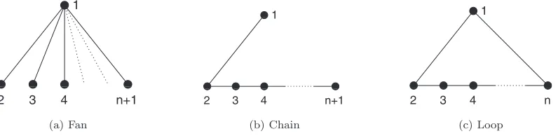
E共兩Aij兩X兲=Cij. 共16兲 It will also turn out to be convenient to define the following sequences of higher-order connectivity moments, which we may associate with the network structural “motifs”关19兴 sug-gested by their respective descriptions共Fig.1兲:

0

0

1

1

010 0 0 0 0 010 0 0 0 0 0 0 0 0 0 0 0 0 0 0 0 0 0 0 0 0 0 0 0 0 0 0 0 0 0 0 0 0 0 0 0 0 0 0 0 0 0 0 0 0 0 0 0 0 0 0 0 0 0 0 0 0 0 0 0 0 0 0 0 0 0 0

1 1 1 1 1 1 1 1 1 1 1 1 1 1 1 1 1 1 1 1 1 1 1 1 1 1 1 1 1 1 1 1 1 1 1 1 1 1 1 1 1 1 1 1 1 1 1 1 1 1 1 1 1 1 1 1 1 1 1 1 1 1 1 1 1 1 1 1 1 1 1 1

0 0 0 0 0 0 0 0 0 0 0 0 0 0 0 0 0 0 0 0 0 0 0 0 1 1 1 1 1 1 1 1 1 1 1 1 1 1 1 1 1 1 1 1 1 1 1 1

0 0 0 0 0 0 0 0 0 0 0 0 0 0 0 0 0 0 0 0 0 0 0 0 0 0 0 0 0 0 0 0 0 0 0 0 0 0 0 0 0 0 0 0 0 0 0 0 0 0 0 0 0 0 0 0 0 0 0 0

1 1 1 1 1 1 1 1 1 1 1 1 1 1 1 1 1 1 1 1 1 1 1 1 1 1 1 1 1 1 1 1 1 1 1 1 1 1 1 1 1 1 1 1 1 1 1 1 1 1 1 1 1 1 1 1 1 1 1 1

1

2 3 4 n+1

(a) Fan

01

010 0 001 0 0 010 01 0 0 0 0 0 0

0 0 0 0 0 0 0 0 0 0 0 0 0 0 0 0 0 0 0 0 0 0 0 0 0 0 0 0 0 0 0 0 0 0 0 0 0 0 0 0 0 0 0 0 0 0 0 0 0 0 0 0 0 0 0 0 0 0 0 0 0 0 0 0 0 0

1 1 1 1 1 1 1 1 1 1 1 1 1 1 1 1 1 1 1 1 1 1 1 1 1 1 1 1 1 1 1 1 1 1 1 1 1 1 1 1 1 1 1 1 1 1 1 1 1 1 1 1 1 1 1 1 1 1 1 1 1 1 1 1 1 1 1 1 1 1 1 1 1 1 1 1 1 1 ₁

2 3 4 n+1

(b) Chain 0 0 1 1 0 0 1 1 0 0 1 1

01 0011 0 0 0 0 0 0

0 0 0 0 0 0 0 0 0 0 0 0 0 0 0 0 0 0 0 0 0 0 0 0 0 0 0 0 0 0 0 0 0 0 0 0 0 0 0 0 0 0 0 0 0 0 0 0 0 0 0 0 0 0 0 0 0 0 0 0 0 0 0 0 0 0 0 0 0 0 0 0

1 1 1 1 1 1 1 1 1 1 1 1 1 1 1 1 1 1 1 1 1 1 1 1 1 1 1 1 1 1 1 1 1 1 1 1 1 1 1 1 1 1 1 1 1 1 1 1 1 1 1 1 1 1 1 1 1 1 1 1 1 1 1 1 1 1 1 1 1 1 1 1 1 1 1 1 1 1

0 0 0 0 0 0 0 0 0 0 0 0 0 0 0 0 0 0 0 0 0 0 0 0 0 0 0 0 0 0 0 0 0 0 0 0 0 0 0 0 0 0 0 0 0 0 0 0 0 0 0 0 0 0 0 0 0 0 0 0 0 0 0 0 0 0 0 0 0 0 0 0 0 0 0 0 0 0 0 0 0 0 0 0 0 0 0 0 0 0 0

1 1 1 1 1 1 1 1 1 1 1 1 1 1 1 1 1 1 1 1 1 1 1 1 1 1 1 1 1 1 1 1 1 1 1 1 1 1 1 1 1 1 1 1 1 1 1 1 1 1 1 1 1 1 1 1 1 1 1 1 1 1 1 1 1 1 1 1 1 1 1 1 1 1 1 1 1 1 1 1 1 1 1 1 1 1 1 1 1 1 1

2 3 4 n

1

[image:3.612.110.508.58.155.2]

(c) Loop

Fan moments: ␮n⬅E共C12C13. . .C1,n+1兲,

n= 1,2, . . . ,N− 1; 共17a兲

Chain moments: ␯n⬅E共C12C23. . .Cn,n+1兲, n= 1,2, . . . ,N− 1; 共17b兲

Loop moments: ␻n⬅E共C12C23. . .Cn,1兲, n= 3,4, . . . ,N. 共17c兲 Since theCijare bounded all expectations are guaranteed to exist. Note too that the labeling of nodes 1 , 2 , . . . is arbi-trary共and, since theXiare iid, irrelevant兲. This construction might be generalized to arbitrary motifs as follows: if G is any graph, then we could define␮共G兲 to be the appropriate expectation over all subgraphs of our network isomorphic to G.

We have the identities

␮1⬅␯1⬅␮, 共18兲

␮2⬅␯2=␳␴2+␮2. 共19兲

III. STATISTICAL PROPERTIES OF SERN ENSEMBLES

A. The large network limit

As mentioned in Sec. I, we shall be concerned chiefly with the connectivity statistics of “large” networks. More precisely, we consider limiting properties of sequences of SERN ensembles of sizeNasN→⬁. For such sequences we restrict ourselves to the case where both the underlying met-ric spaceS,d共· , ·兲and node distributionXare held fixed关28兴

and only the decay function␥共s兲is scaled with network size. In the passage to the limit we follow common共but not exclusive兲practice in network theory and keep themean de-greeof nodes fixed. We shall see in the next section that for a SERN ensemble ofN nodes this is just共N− 1兲␮; we thus introduce themean degreeparameter:

␬⬅ 共N− 1兲␮. 共20兲

Now, unlike Erdös-Rényi random graphs where we have a single real-valued scale parameter p, scaling a SERN en-semble involves scaling afunction ␥共s兲with potentially in-finite degrees of freedom. There is therefore no unique “ge-neric” scaling mode; rather, for given mean degree␬, scaling of connectivity with increasing network size requires a se-quence of decay functions ␥N:R+→关0 , 1兴 under the con-straint that␬ be held constant. By abuse of terminology, in referring to “a large SERN ensemble”共cf. Sec. I兲, it is to be understood that such a scaling sequence is implicit, although in the interests of notational brevity we generally suppress the subscriptN.

We return to the topic of scaling later; we shall see that network structure in the large network limit may depend cru-cially on the precise scaling model共cf. Sec. IV兲.

B. Degree distribution

Let the rv

Ki⬅

兺

j

Aij 共21兲

共i= 1 , . . . ,N兲denote the degree of nodei. TheKiare identi-cally共but not independently兲distributed as K, say. We thus find immediately that the mean degree of a randomly se-lected node is

E共K兲=共N− 1兲␮=␬. 共22兲 More generally, the joint probability generating function 共pgf兲 关29兴of theKiis

G共z1, . . . ,zN兲=E共z1 K₁

. . .zN K_N兲

=E

冉

兿

i_⬍j

共zizj兲Aij

冊

=E

冉

兿

i_⬍j

关1 −共1 −zizj兲Cij兴

冊

.

共23兲 The pgf for the degree of an arbitrary node共node 1, say兲may be calculated as follows:

G共z兲=E

冉

兿

1⬍j

关1 −共1 −z兲C1j兴

冊

=E

冠

E

冉

兿

1⬍j

兩关1 −共1 −z兲C1j兴兩X1

冊冡

共24兲

=E

冉

兿

1⬍j

关1 −共1 −z兲E共兩C1j兩X1兲兴

冊

共25兲

=E共关1 −共1 −z兲E兩„c共X,Y兲兩X…兴N−1_{兲, 共26兲} withYiid asX. At step共24兲we condition onX₁; at step共25兲

we use the fact that theC1jgivenX1 are independent and at step共26兲that theE共C1j兩X1兲are all equal toE(c共X,Y兲兩X). It is now convenient to introduce the function:

␸共x兲 ⬅E„c共x,Y兲…, 共27兲 which represents the mean connectivity for a node atx苸S and we define theconditional mean degreeto be the random variable:

⌫⬅ 共N− 1兲␸共X兲=共N− 1兲E„c兩共X,Y兲兩X…. 共28兲

We may then write, Eq.共26兲as

G共z兲=E

冉

冋

1 − 1

N− 1共1 −z兲⌫

册

N−1

冊

. 共29兲

⌫completely determines the degree distribution. Intuitively, ⌫describes how mean node degree varies with location of a node inS. In particular关cf. Eq.共25兲below兴itsvariancemay be considered a measure of the “spatial inhomogeneity” of connectivity of a SERN ensemble. Thenth moment of⌫ is given by

E共⌫n兲=共N− 1兲n␮n=␬n

␮n

␮n, 共30兲

where␮nis thenthfan moment共17a兲. In particular,

var共⌫兲=共N− 1兲2␳␴2=␬2

冉

␮2

␮2− 1

冊

共31兲

and we see immediately that if the connectivity correlation␳ vanishes then ⌫ has zero variance and is 共almost surely兲 constant. The degree distribution is then binomially distrib-uted and we might expect such networks to behave some-what like random graphs; but note that statistical properties 共such as clustering兲 which do not derive purely from the degree distribution may not be assumed to be as for random graphs. A particular situation where connectivity correlation vanishes is described in the next section.

In the largeNlimit, provided limN→⬁⌫ exists,

G共z兲→E共e−共1−z兲⌫兲, 共32兲 so that thedegree distributionof a SERN ensemble is given by

P共K=k兲→ 1 k!E共⌫

k_e−⌫_{兲 共33兲} fork= 0 , 1 , 2 , . . ..

Two further technical results are stated here as follows: Proposition 1.In the large network limit:

兺

j⫽i

Cij→⌫ 共34兲

in distribution for any i. Proof. We have

G共z兲=E共e兺j⫽iln共1−共1−z兲Cij兲兲, 共35兲

→E共e−共1−z兲兺j⫽iCij兲, 共36兲

for large N, since the individual Cij→0. Comparing with 共32兲and noting thatG共z兲is justM_⌫共z− 1兲, whereM_⌫共t兲is the moment generating function for ⌫, the result follows from

the continuity theorem关29兴.

Proposition 2. Let the rv ⌳ be the largest eigenvalue of the connectivity matrixC. Then in the large network limit, ⌳→⌫in distribution.

Proof. Since C is real, symmetric and presumably non-zero, the Perron-Frobenius theorem tells us that such a real-valued⌳exists and is associated with a real, positive 共ran-dom兲 eigenvector V=共V1, . . . ,VN兲, say. Then 兺jCijVj=⌳Vi and summing over i we have 共兺iVi兲⌳=兺i,jCijVj. But from Proposition 1 we have兺iCij→⌫ and the result follows. As an example, if the decay function␥共s兲is const=␮, so that our ensemble is a simple random graph withCij=␮for all i⫽j, then the characteristic equation for C is 共⌳ +␮兲N−1关⌳−共N− 1兲␮兴= 0 so that ⌳=␬=⌫ in the large net-work limit.

C. Special SERN ensembles

At this point we introduce some subclasses of SERN en-sembles with specialized spatial/statistical properties.

1. Poisson ensembles

From Eqs.共31兲and共32兲we see that if limN→⬁⌫exists and var共⌫兲→0 共equivalently ␮2

␮2→1兲 as N→⬁ then the degree

distribution tends towards a Poisson distribution with param-eter␬. We shall call such an ensemblePoisson. Note that it is not sufficient merely that␳→0 共cf. Sec. V兲.

2. Uniform ensembles

We describe a SERN ensemble as uniform if the node distributionXis uniform; it follows that the underlying space Smust then have finite measure.

3. Spatially homogeneous ensembles

We describe a SERN ensemble as 共spatially兲 homoge-neous if ∀x,y苸S there exists an isometry ␾:S→S of S 共i.e., metric-preserving 1 − 1 mapping ofS onto itself兲 that mapsxtoyand such that␾共X兲has the same distribution as X. Since an isometry preserves the volume element onS, it is necessary 共but not sufficient兲 that the ensemble be uni-form.

Proposition 3. Let Y be iid as X.Then if the network is homogeneous X and d共X,Y兲 are independent.

Proof.Pick some fixedx0苸S. Then for anyx苸Swe can find an isomorphism␾such that␾共x兲=x₀. For anya苸R+_we have

P„d共x,Y兲ⱕa…=P共d„x0,␾共Y兲…ⱕa兲=P共d共x0,Y兲ⱕa兲. Thus the distribution ofd共x,Y兲does not depend onxand the

result follows.

Proposition 4. Let Y,Z be iid X. Then if the network is homogeneous d共X,Y兲and d共X,Z兲are independent.

Proof. Let dV共x兲 be the volume element on S. For any a,b苸R+_{we have}

P„d共X,Y兲ⱕa,d共X,Z兲ⱕb…

=

冕

S

P„d共x,Y兲ⱕa,d共x,Z兲ⱕb…dV共x兲

=

冕

S

P„d共x,Y兲ⱕa…P„d共x,Z兲ⱕb…dV共x兲

by independence of Y, Z. But from Proposition 3, P(d共x,Y兲ⱕa)=P(d共X,Y兲ⱕa)∀xand the result follows.

Corollary. If a SERN ensemble is homogeneous then the connectivity correlation␳ vanishes.

In particular, a homogeneous ensemble is Poisson pro-vided that limN→⬁⌫ exists.

We thus see共cf. Sec. III C 5 below兲thatspatial symmetry imposes a rather severe constraint on network structure.

4. Uniformly continuous ensembles

continu-ous, but not uniformly so. We note that anyuniform 共and in particular anyhomogeneous兲ensemble is uniformly continu-ous共see also Sec. V A兲.

5. Scale free ensembles

Following the argument in 关15兴 we find that the degree distribution of a SERN ensemble will be scale free iff there is somemⱖ1 such thatE共⌫n_{兲 diverges for alln⬎min the} large network limitN→⬁. From Eqs.共30兲and共20兲we thus have:

Proposition 5. A SERN ensemble is scale free iff∃mⱖ1 such that for all n⬎m, ␮n

␮n→⬁ as N→⬁.

Clearly a Poisson ensemble cannot be scale free. In关15兴it is demonstrated that scale free spatial networks do indeed exist; see also our Example 2 of Sec. V C.

6. Generalized random geometric graphs

Spatial network models withtruncation decay:

␥共s兲 ⬅

再

1, 0ⱕs⬍r

0, rⱕs 共37兲

so thatr→0 asN→⬁have been quite widely studied in the literature—albeit exclusively for flat manifolds with uniform node distribution—as random geometric graphs 共RGGs兲 关13,14兴. Frequently, the emphasis has been on analysis of

thresholdsfor the appearance of various structural properties, often using sophisticated techniques from continuum perco-lation theory. We generalize RGGs to arbitrary SERN en-sembles with truncation decay; that is,S may be any Rie-mannian manifold and the node distribution X is not necessarily uniform. Generalized random geometric graphs 共GRGGs兲offer the possibility of being far more tractable to analysis than SERN ensembles in full generality; this is largely down to the observation that as N→⬁ we always average quantities increasingly locally. We shall examine GRGGs in more detail in Sec. V.

D. Clustering coefficient

Our definition of clustering coefficient C will be “the probability that a random triplet of distinct nodes form a triangle, given that it form an ‘elbow’ ”—this corresponds to the共more or less兲standard version of

C⬅3⫻no. of triangles no. of “elbows”

—but, we note there are two feasible ways to average this quantity over a SERN ensemble:共i兲for a given node distri-bution X we construct the clustering coefficient for the 共sub兲ensemble with node distribution X—then we average the coefficients overX. 共ii兲 node triplets are sampled from ensembles withdifferentnode distributions. Here we choose the second definition as being by far the easier to calculate, both analytically and in Monte Carlo simulation. Without loss of generality we label the nodes 1, 2, and 3 共with the “elbow” at node 1兲so that

C⬅P共兩A23= 1兩A12= 1,A13= 1兲=

␻3

␮2

, 共38兲

that is, the third loop moment divided by the second fan moment.

E. Degree correlation

Firstly, we calculate the conditional mean degree of an arbitrary node; i.e., for k= 0 , 1 , 2 , . . . we calculate the mean degree␬¯共k兲of an arbitrary node conditional on it being con-nected to a node of degreek. Without loss of generality we take the nodes to be labeled 1 and 2. We then have

␬

¯共k兲 ⬅E共兩K2兩A12= 1,K1=k兲. 共39兲

Let us define the joint conditional generating functions 共cf. 关24兴兲:

G共z1,z2兲 ⬅

兺

k₁,k₂

P共兩K1=k1,K2=k2兩A12= 1兲z1 k₁

z₂k2_. 共40兲

Analogously to Eq.共27兲, we define

␺共x,y兲 ⬅E„c共x,Z兲c共y,Z兲… 共41兲 forx,y苸S, whereZ iid asX. Using the shorthand notation

C⬅c共X,Y兲, 共42兲

⌽1⬅␸共X兲, 共43兲

⌽2⬅␸共Y兲, 共44兲

⌿⬅␺共X,Y兲, 共45兲

we may then calculate

␮G共z1,z2兲=z1z2E„C关1 −⌽1共1 −z1兲−⌽2共1 −z2兲 +⌿共1 −z1兲共1 −z2兲兴N−2…. 共46兲 Setting

gk共z兲 ⬅

冏

1 k!

⳵k G共z1,z兲

⳵z₁k

冏z

1=0

, 共47兲

we may now verify that

␬

¯共k兲=gk

⬘共

1兲 gk共1兲

, 共48兲

and we have

␮gk共z兲=

冉

N− 2

k− 1

冊

zE„C关⌽1−⌿共1 −z兲兴 k−1

⫻关1 −⌽1−共⌽2−⌿兲共1 −z兲兴N−k−1…, 共49兲

so that

␮gk共1兲=

冉

N− 2

k− 1

冊

E„C⌽1

␮gk

⬘共1兲

=␮gk共1兲+

冉

N− 2

k− 1

冊

共k− 1兲E„C⌿⌽1

k−2_{共1 −⌽1兲}N−k−1_…

+

冉

N− 2

k− 1

冊

共N−k− 1兲E„C共⌽2−⌿兲 ⫻⌽1

k−1_{共1 −⌽1兲}N−k−2_{…. 共51兲}

Let us now define

Pk共x兲 ⬅P共兩K=k兩X=x兲= 1

k!关共N− 1兲␸共x兲兴 k

e−共N−1兲␸共x兲 共52兲 forx苸S and set

␯2关k兴 ⬅E„c共Y,Z兲c共X,Y兲Pk−1共X兲…, 共53兲

␻3关k兴 ⬅E„c共Y,Z兲c共X,Y兲c共X,Z兲Pk−2共X兲…. 共54兲 We may think of these as “degree conditional” versions of the corresponding connectivity moments. In the largeNlimit 共withkN兲we then find that

␬

¯共k兲 ⬇1 +N2␯2关k兴+␻3关k兴−␻3关k+ 1兴

kP共K=k兲 . 共55兲 We may express the 共conditional兲 degree correlation in terms of partial derivatives of the generating function共40兲at z1=z2= 1. It may then be calculated from Eq. 共46兲 to yield 共approximately for largeN兲

corr共兩K₁,K2兩A₁₂= 1兲 ⬇␩1␬+C

␩2␬+ 1

, 共56兲

where we define

␩1⬅

␮␯3−␮22

␮2_␮ 2

, 共57兲

␩2⬅

␮␮3−␮22

␮2_␮ 2

. 共58兲

We note firstly that the clustering coefficientCis alwaysⱖ0;

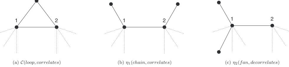
␩2ⱖ0 follows from the Cauchy-Schwartz inequality 关29兴, noting that␮n=E(␸共X兲n). In the general case, ␩1 might be negative. Figure 2 illustrates the effects of the factors C,␩1,␩2 entering into the expression共56兲 for degree lation. Clustering is associated with increased degree

corre-lation via shared edges creating a loop; ␩2 corresponds to small fans emanating from one of the connected nodes, de-creasing degree correlation.␩1 corresponds to short chains passing through the connected nodes, affecting degree corre-lation according to the sign of␩1. We note that in the Poisson case␩2⬅0, so that the conditional degree correlation is just

␩1␬+C. In general, we might say intuitively that while clus-tering exerts a “homogeneous” correlating effect on degree, “inhomogeneity”共in the sense of spatial variation of connec-tivity兲 exerts an effect on degree correlation via thecoeffi-cients␩₁,␩₂共see in particular Sec. V A below兲. We note that a necessary condition that degree correlation be dis assorta-tive is that␩1⬍0. It is not clear under what conditions this might occur; in Sec. V A we shall see that for uniformly continuous GRGGs 共and, we conjecture, in fact for any GRGG兲we have␯n=␮nfor alln, so that␩1=␩2 and degree correlation is always assortative.

F. Giant component

For their “configuration model” Newman et al. 关18,31兴

developed a powerful generating function formalism to derive—amongst other things—approximations for the phase transition to the appearance of a giant component and the size of the giant component beyond the phase transition. We cannot apply this formalism mutatis mutandis for two rea-sons: firstly—unlike the configuration model—node degrees 共conditional on node distribution兲are neither identically nor independently distributed for SERN ensembles. Secondly, the formalism depends on neglecting the probability of loops in small components; since SERN ensembles may well fea-ture significantclusteringthis assumption is likely to be non-viable.

As an example, in关31兴the following argument is used to derive the size of the giant component for the configuration model in the large network limit: assume there is a giant component and defineuto be the probability that an arbitrary node doesnotbelong to the giant component. Then none of that node’s neighbors must belong to the giant component, leading to the “consistency relation”:

u=G共u兲, 共59兲 whereG共z兲 is the generating function for node degree共29兲.

We can then—at least in principle—solve Eq. 共59兲 for u 共apart from the trivial solution u= 1兲. The problem in our case is that in deploying this procedure naively we disregard

01

01

0 0 0 0 0 0 0 0 0 0 0 0 0 0 0 0 0 0 0 0 0 0 0 0 0 0 0 0 0 0 0 0 0 0 0 0 0 0 0 0 1 1 1 1 1 1 1 1 1 1 1 1 1 1 1 1 1 1 1 1 1 1 1 1 1 1 1 1 1 1 1 1 1 1 1 1 1 1 1 1

0 0 0 0 0 0 0 0 0 0 0 0 0 0 0 0 0 0 0 0 0 0 0 0 0 0 0 0 0 0 1 1 1 1 1 1 1 1 1 1 1 1 1 1 1 1 1 1 1 1 1 1 1 1 1 1 1 1 1 1

1 2

(a)C(loop, correlates)

01

01 01

0 0 0 0 0 0 0 0 0 0 0 0 0 0 0 0 0 0 0 0 0 0 0 0 1 1 1 1 1 1 1 1 1 1 1 1 1 1 1 1 1 1 1 1 1 1 1 1

0 0 0 0 0 0 0 0 0 0 0 0 0 0 0 0 0 0 0 0 0 0 0 0 1 1 1 1 1 1 1 1 1 1 1 1 1 1 1 1 1 1 1 1 1 1 1 1

1 2

(b)η1(chain, correlates)

01 01 01 0 0 1 1

0 0 0 0 0 0 0 0 0 0 0 0 0 0 0 0 0 0 0 0 0 0 0 0 1 1 1 1 1 1 1 1 1 1 1 1 1 1 1 1 1 1 1 1 1 1 1 1 0 0 0 0 0 0 0 0 0 0 0 0 0 0 0 0 0 0 0 0 0 0 0 0 0 0 0 0 0 0 1 1 1 1 1 1 1 1 1 1 1 1 1 1 1 1 1 1 1 1 1 1 1 1 1 1 1 1 1 1

1 2

[image:7.612.61.551.60.175.2]

(c)η2(f an, decorrelates)

the fact that given a particular node distributionXthe prob-ability that a node belong to the giant component will vary with the choice of node. We should not be surprised, then, that Eq.共59兲yields in general a poor approximation foru. In the large network limit Eq.共59兲becomes

u=E共e−共1−u兲⌫兲. 共60兲 For Poisson ensembles in particular, we have ⌫= const=␬ and Eq.共60兲becomes in the large network limit:

u=e−␬共1−u兲 _共61兲 which may be solved in terms of 共the principal branch of兲 Lambert’sW function as

u= −1

␬W共−␬e−␬兲 ⬇

1

␬e1−␬, 共62兲

which suggests, among other things, a phase transition at␬ = 1 as for Erdös-Rényi random graphs; however, as demon-strated in 关14兴 for uniform random geometric graphs 共see Sec. V兲on Euclidean space there is indeed a phase transition to the appearance of a giant component, but the critical con-nectivity in fact varies withspatial dimension, with the tran-sition at␬= 1 the limiting value for large dimension. In ef-fect, clustering—which decreases with increasing dimension 关14兴—renders the procedure inaccurate.

A more exact approach to the “consistency relation” argu-ment runs as follows共see also 关22兴for a more precise deri-vation for a comparable model兲: given a node distributionX let Ui—now jointly distributed with X—be the probability that node i does not belong to the giant component. The consistency relation then becomes

Ui=e−兺jCij共1−Uj兲. 共63兲 If we could extract a共possibly approximate兲algebraic solu-tion of Eq.共63兲considered as a set of simultaneous equations for theUithen we could in principle calculateu=E共Ui兲; this would appear to be difficult, however, and we have not suc-ceeded in doing so.

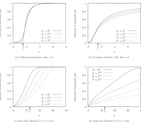
We in fact conjecture that, contrary to common assump-tion, for general SERN ensembles there is a phase transition only in the case of uniform ensembles; for all other en-sembles, the fraction of the network occupied by the largest component increases smoothly with increasing mean connec-tivity␬. Intuitively, inhomogeneity in the spatial distribution of nodes induces a clustering of connectivity around regions of higher node density, which “smears out” the transition in the following sense: for a fixed node distribution 共63兲 may yield a critical mean connectivity value, but this value will depend on the particular node distribution so that criticality is obliterated by the averaging process. This intuition is con-firmed in all simulations we have performed with nonuni-form ensembles关32兴 共see, e.g., Sec. V and Fig.5兲.

A further subtlety arises in that simulations suggest that if mean connectivity␬is below the phase transition, or if there is no phase transition, then共holding␬ fixed兲the fraction of the network occupied by the largest component actually shrinks as N→⬁; effectively, the network “breaks up” as network size increases.

G. Mean path length

We need to consider carefully what exactly we intend by “mean path length”; we would like to define thepath length random variableL to be the minimum number of edges we need to traverse to connect two共distinct兲randomly selected nodes in a random instantiation of our ensemble. But note that there may benopath connecting the nodes共specifically when the nodes lie in different components兲; in this case it is customary, by abuse of terminology, to refer to the path length as “infinite,” so that L takes values in 兵1 , 2 , . . . ,N − 1 ,⬁其. The most common approach is to take the condi-tional arithmetic meanE共L兩L⬍ ⬁兲; that is, we take the mean over those pairs of distinct nodes for which a connecting path exists. An alternative共and arguably better兲approach is to consider instead the harmonic mean1/E共1/L兲, which is well defined if we define 1/L⬅0 where there is no connect-ing path.

We note that

P共L⬍ ⬁兲ⱖ共1 −u兲2, 共64兲 whereuis as in the previous section; i.e., 1 −uis the fraction of the network occupied by the largest component. We note that, as for the fraction of the network occupied by the larg-est component 共see previous section兲 P共L⬍ ⬁兲 actually shrinks asN→⬁; nonetheless, in all cases we have examined in simulation mean path length共both conditional arithmetic or harmonic兲still appears to increase with network size.

Following关33兴we may calculate the probability: P共L= ᐉ兲=F_ᐉ−F_ᐉ−1 共65兲 forᐉ= 1 , 2 , . . . ,N− 1 in the large network limit, where

F_ᐉ⬅1 −E_„exp共−关Cᐉ兴12兲_… 共66兲 共andF₀⬅0兲yielding

P共L⬍ ⬁兲=FN−1, 共67兲

E共兩L兩L⬍ ⬁兲=N−

兺

ᐉ=1 N−1

F_ᐉ/FN−1. 共68兲

Now in关33兴a specialization of the “hidden variable” model introduced in关24兴is analyzed in which the equivalent of our Cij factorizes into the product of independent random vari-ables. This allows the summation in Eq.共68兲to be calculated via the Poisson summation formula 关30兴; in our case the

nonseparability of the Cij would seem to preclude this ap-proach and it is not clear how we should calculate either Eq. 共68兲or indeed Eq.共67兲.

IV. SMALL WORLD SERN ENSEMBLES

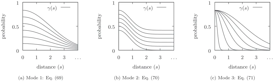
decay, where nodes are connected iff they lie within a given distance共cf. Sec. V兲,linear decay,exponential decay,power law decay, etc. Some intuitively “natural” ways to derive a sequence of decay functions from a base decay function in order to define a large network limit are共Fig.3兲:

共1兲Reduce the connection probability by a constant fac-tor:

␥N共s兲 ⬅␭N␥ˆ共s兲 共69兲 and let␭N→0 asN→⬁ so as to maintain␬= const.

共2兲 Reduce the connection probability by a constant amount:

␥N共s兲 ⬅␥ˆ共s兲−共␥ˆmin−cN兲 共70兲 关where␥ˆmin is the minimum value of ␥ˆ共s兲over its domain兴 and letcN→0 asN→⬁so as to maintain␬= const; but note that this imposes a limit on the largest possibleN.

共3兲 Let characteristic decay length tend to zero 共i.e., shrink the distance at which connections appear with given probability兲:

␥N共s兲 ⬅␥ˆ

冉

s rN

冊

共71兲

and letrN→0 as N→⬁, again while holding␬ constant. Now Watts and Strogatz originally defined “small world” to mean not just sublogarithmic scaling of mean path length with network size, but also nonvanishing of the clustering coefficient in the large network limit关2兴. It is immediately

evident from Eq.共69兲that scaling according to mode 1 above will result in a vanishing clustering coefficient, since any connectivity moment of ordernclearly scales as␭Nn. Mode 2 does not allow us to takeNto arbitrarily large size. For mode 3 we might well expect 共and simulation bears this out兲 a nonzero clustering coefficient since “triangles” of nodes that fall entirely within the connectivity radius will be fully con-nected. However, the following heuristic argument suggests that scaling according to mode 3 might also be expected to lead to power law rather than logarithmic decay of mean path length.

Suppose then that a decay function␥共s兲 has the property that ␥共s兲= 0 for s⬎r, say; that is, there will be no connec-tions for nodes further apart than共spatial兲distancer. Let the random variable D⬅d共X,Y兲, jointly distributed with mean

path lengthL, be the distance between random nodes X,Y. We attempt to derive a lower bound on mean path length based on the observation that for any r and ᐉ= 1 , 2 , . . . ,N − 1:

D⬎ ᐉr⇒L⬎ ᐉ, 共72兲 i.e., if two nodes are a greater distance thanᐉrapart, then it takes at leastᐉ+ 1 edges to link them. From this we deduce that for the conditional arithmetic mean

E共兩L兩L⬍ ⬁兲ⱖ1

rE共兩D兩L⬍ ⬁兲 共73兲

if the conditional meanE共D兩L⬍ ⬁兲exists. This is, perhaps, not terribly useful except for the case where mean connec-tivity is beyond a phase transition to formation of a giant component, in which case we may treat the term E共D兩L ⬍ ⬁兲as constant. Similarly we find for the harmonic mean

1 E共1/L兲ⱖ

1 r

1

E共1/D兲 共74兲

again providedE共1/D兲exists关34兴.

In either case, within the 共admittedly rather restrictive兲 provisos outlined above, we see that path length scales at least as 1_r. Suppose now that a base decay function ␥ˆ共s兲 satisfies␥ˆ共s兲= 0 fors⬎1, say. We then have

␮=r

冕

0 1

␥ˆ共s兲共rs兲ds, 共75兲

where共s兲 is the density of d共X,Y兲, so that if 共s兲 is rea-sonably well behaved we have approximately, for smallr:

␮⬀r␤ 共76兲

for some␤⬎0 and, since we hold␬⬅共N− 1兲␮fixed, we see from Eq.共73兲 关respectively,共74兲兴that conditional arithmetic 共respectively, harmonic兲path length scales at least asN1/␤_as N→⬁; in particular, it grows faster than logarithmically, so that our network cannot be small world. We conjecture that this is in fact always the case if connectivity decays accord-ing to mode 3; simulations of various SERN ensembles 共in-cluding severely singular node distributions兲under this scal-ing mode bear out this conclusion.

0 0.5 1

0 1 2 3 . . .

p

rob

ab

ilit

y

distance (s)

γ(s)

(a) Mode 1: Eq. (69)

0 0.5 1

0 1 2 3 . . .

p

rob

ab

ilit

y

distance (s)

γ(s)

(b) Mode 2: Eq. (70)

0 0.5 1

0 1 2 3 . . .

p

rob

ab

ilit

y

distance (s)

γ(s)

[image:9.612.70.551.56.200.2]

(c) Mode 3: Eq. (71)

To summarize: reducing connection probability by a con-stant factor may well result in mean path length scaling sub-logarithmically with network size, but implies a vanishing clustering coefficient. Reducing connection probability by a constant amount does not allow passage to a large network limit. Shrinking the connection radius may well yield a non-zero clustering coefficient, but is likely to lead to superloga-rithmic scaling of mean path length.

There is, however, a suggestion in 关14兴 that we may achieve small world behaviour in the sense of Watts and Strogatz by deploying acombinationof scaling modes 共see also 关12,35兴兲. We demonstrate a construction along these lines in the following section.

Construction of small world ensembles

Consider the behavior of the clustering coefficient for a decay function sequence:

␥

˜N共s兲 ⬅ 共1 −qN兲␥N共s兲+qN, 共77兲 where␥N共s兲 is a given decay function sequence yielding a nonzero clustering coefficient CN→C⬎0 in the limit and qN→0 as N→⬁. Indeed, if the ␥N共s兲 are truncation decay 共cf. Sec. V兲, the resulting ensemble may be thought of as a continuous analog of the original Watts-Strogatz model: a small decay radius r leads to latticelike local connectivity, while a uniform connection probabilityqcorresponds to ran-dom distance-independent 共hence potentially long range兲 connections. We wish to determine firstlyhowwe may take qN→0 in order that the clustering coefficient ˜C tend to a nonzero limit. We wish to establish in addition whether ap-propriate qN scaling can yield sublogarithmically scaling 共i.e., small world兲mean path length.

Denoting quantities corresponding to the decay function 共77兲by a tilde 共from here forward we drop the subscript N for notational clarity兲, we have

␸

˜共x兲=共1 −q兲␸共x兲+q 共78兲 forx苸S, and

␮

˜ =共1 −q兲␮+q, 共79兲

␮˜₂=共1 −q兲2␮2+ 2q共1 −q兲␮+q2, 共80兲

␻˜₃=共1 −q兲3␻3+ 3q共1 −q兲2␮2+ 3q2共1 −q兲␮+q3. 共81兲 Setting␭⬅␮2/␮2 we may calculate

C

˜_{−␮˜ =}共1 −q兲␭共C−␮兲+ 2q共␭− 1兲

␭− 1 +共1 +₁₋q/␮_q2_兲 . 共82兲 In the large network limit and assuming C→const⬎0 we have

C

˜_→ ␭C+ 2q共␭− 1兲

␭− 1 +共1 +q/␮2兲 共83兲 and we may state

Proposition 6. In the large network limit N→⬁, if C →const⬎0 then˜C→const⬎0 iff:

I . ␭→const⬎0 and q

␮→c

so that C˜→ ␭

␭− 1 +共1 +c兲2C 共84兲

or II . ␭→ ⬁ and

_冑

q

␮2

→c

so that C˜→ 1

共1 +c兲2C 共85兲 for some constant cⱖ0.

It follows that if C→const⬎0 we may always scale q with␮so that˜C→const⬎0 and␮˜→0 as required. We note that Case I covers Poisson ensembles, where␭⬅1.

We also note from Eq.共78兲that if our original ensemble is Poisson, then so is the derived small world ensemble. We may calculate for Case I that

␮˜n

␮˜n→共1 +c兲 −n

兺

k=0 n

冉

n

k

冊

c n−k␮k

␮k, 共86兲

so that the derived small world ensemble is scale free iff the original ensemble is scale free, while for Case II:

␮˜n

␮˜n→

兺

k=0 n

冉

n

k

冊

c −k ␮k

共

冑

␮2兲k, 共87兲

so that the derived small world ensemble is scale free iff∃n₀ such that␮n/共

冑

␮2兲ndiverges for alln⬎n0.

We now turn to mean path length scaling asN→⬁, hold-ing mean degree fixed. Now it is clear from Eq. 共79兲 that, given fixed mean degree˜␬⬅N␮˜ the mean path length for the new ensemble satisfies

E„L共␬˜,N兲…ⱕE„LRG共Nq,N兲…, 共88兲 whereLRG denotes path length for an Erdös-Rényirandom graph 关36兴, since the additional connection probability 共1 −q兲␮in Eq.共79兲can onlydecreasemean path length. Now for Case I,q→c␮ for some constantc, so that in the large network limit we find thatq⬇₁₊c_c␮˜, so that

E„L共␬˜,N兲…ⱕE

冠

LRG

冉

c

1 +c˜␬,N

冊冡

. 共89兲 Since we know that mean path length for a random graph scales logarithmically with network size, it follows that so too does E(L共␬˜,N兲) and the new ensemble is indeed small world. For Case II we find thatq⬇␮˜ for largeNso that

E„L共␬˜,N兲…ⱕE„LRG共˜␬,N兲…, 共90兲 and the new ensemble is again seen to be small world.

V. GENERALIZED RANDOM GEOMETRIC GRAPHS

共Sec. III C 6兲, illustrating our analysis with some examples. We note here that for GRGGs we always have

␴2_{⬅␮共1 −␮兲 ⬇␮ 共91兲}

in the large network limit.

A. Uniformly continuous GRGGs

Suppose we have a uniformly continuous GRGG 共Secs. III C 4 and III C 6兲on a closed, orientedm-dimensional Rie-mannian manifold S. Since as N→⬁ we always average quantities increasingly locally we may convince ourselves that to lowest order inr we may approximate our space as Euclidean; that is, to a first approximation curvature of S may be neglected in the large network limit 共this may be demonstrated more rigorously by choosing a Riemann nor-mal coordinate system关37兴locally兲. It is less obvious that if

Shas a sufficiently well-behaved boundary, then the bound-ary makes a negligible contribution to the connectivity mo-ments in the large network limit.

We first consider the boundary-less case. By uniform con-tinuity we have for any ␧⬎0 an r⬎0 such that d共x,y兲 ⬍r⇒兩p共y兲−p共x兲兩⬍␧. Thus,

␸共x兲 ⬅

冕

d_共x,y_兲ⱕr

p共y兲dV共y兲, 共92兲

wheredV共y兲is the volume element in our chosen coordinate system, satisfies

冏

␸共x兲

V共r;x兲−p共x兲

冏

⬍ ␧, 共93兲 where V共r;x兲 represents the volume of a ball of radius r around x. But if r is chosen small enough, then to lowest order inr,V共r;x兲⬇Vm共r兲, where

Vm共r兲=

␲m_/2 ⌫共m

2 + 1兲

rm 共94兲

is the volume of a ball of radiusr in a Euclidean space of dimensionm, and we have

␸共x兲 ⬇Vm共r兲p共x兲 共95兲

to lowest order inr.

Now suppose S has a boundary ⳵S. Let us denote by ⳵S共r兲 the set of points in S of distance at mostrfrom ⳵S. From共95兲we have

␮⬅

冕

S

␸共x兲p共x兲dV共x兲, 共96兲

⬇Vm共r兲E„p共X兲…

−

冕

⳵S共r_兲

关Vm共r兲−V共r;x兲兴p共x兲2dV共x兲.

共97兲

But

冕

⳵S共r兲

关Vm共r兲−V共r;x兲兴p共x兲2dV共x兲ⱕVm共r兲

冕

⳵S共r兲

p共x兲2dV共x兲,

共98兲 and if the boundary is piecewise smooth and we choose r sufficiently small, then

冕

⳵S共r兲

p共x兲2dV共x兲 ⬇r

冕

⳵S

p共x兲2dS共x兲 共99兲

wheredS共x兲 is the volume element on the boundary ⳵S in our chosen coordinate system, so that to lowest order inr:

␮⬇Vm共r兲E„p共X兲…. 共100兲 In the limit of smallr, then, nodes near the boundary make a negligible contribution to␮. The argument extends to higher connectivity moments so that:

Proposition 7. For a uniformly continuous GRGG:

␮n⬇Vm共r兲nE„p共X兲n… 共101兲 for n= 1 , 2 , . . .in the limit N→⬁.

We note firstly that

␮n

␮n→

E„p共X兲n…

E„p共X兲n… 共102兲

in the large network limit, so that

Corollary (1). A uniformly continuous GRGG can never

be scale free.

and secondly, that

␮2

␮2− 1→

var„p共X兲…

E„p共X兲…2 共103兲

in the large network limit, giving:

Corollary (2). A uniformly continuous GRGG is Poisson

iff it is uniform.

It is straightforward to show also that ␯n⬇␮n to lowest order inr for n= 1 , 2 , . . .共we conjecture that this is, in fact, the case for any GRGG兲. Thus to calculate the conditional degree correlation共56兲we have␩1⬅␩₂⬅␩, say, for the co-efficients共57兲and共58兲, which may then be calculated from

Eq.共102兲. As we noted in Sec. III E that␩2ⱖ0 always, we have

Proposition 8. A uniformly continuous GRGG always has assortative degree correlation.

Furthermore, we see that as ␩ increases from zero 共the Poisson or, equivalently, uniform case兲 so the conditional degree correlation共56兲 increases fromC to 1; we might in-terpret this as saying that “inhomogeneity induces additional degree correlation beyond that associated with clustering.”

From Eq.共91兲we also see that

␳= ␮2−␮ 2

The clustering coefficient for RGGs has been computed analytically in关14兴; there they note thatCis independent of network size and共mean兲connectivity. For our GRGGs their result still holds as a limiting case asN→⬁, although it need no longer be constant. They find thatCis always⬎0 and for large dimensionm:

C⬇3

冑

2

␲m

冉

3 4

冊

共m+1兲/2

. 共105兲

We note here that simulations indicate共see, e.g., Fig. 6兲

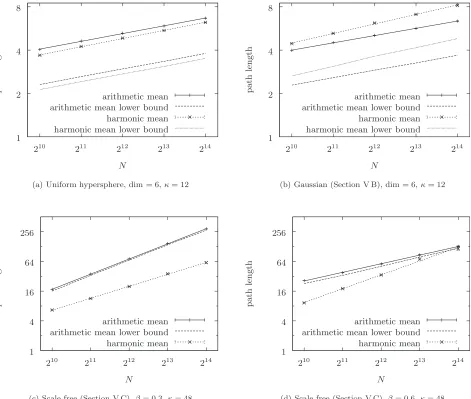
that for GRGGs, mean path length—both conditional arith-metic and harmonic—appears to scale as a power law in network size as suggested by the discussion in Sec. IV and that the exponent is reasonably well predicted by the lower bounds given by Eqs.共73兲and共74兲. We note too that we may

construct a small world ensemble from a uniformly continu-ous GRGG according to the procedure described in Sec. IV; from Eqs.共102兲withn= 2 we see that uniformly continuous GRGGs always fall under Case I of Proposition 6.

B. Example 1: A nonuniform uniformly continuous GRGG

We take the space Rm _{with Euclidean metric and node} distribution with Gaussian density:

p共x₁, . . . ,xn兲=共2␲兲−m/2e−共x1

2

+¯+x_m2兲/2_{. 共106兲} This node distribution is uniformly continuous, but nonuni-form and hence non-Poisson. We may calculate:

␮=P

冉

m 2,

r2

4

冊

, 共107兲

⬇ 2− m ⌫共m

2+ 1兲

rm, 共108兲

for small r 关where P共a,z兲⬅1 −⌫共a,z兲/⌫共a兲 is the comple-mentary normalized incomplete Gamma function兴 and in general:

10−6 10−4 10−2 100

22 24 26 28

d

en

sit

y

degree sampled

Poisson

(a) Uniform hypersphere, dim = 6

10−6 10−4 10−2 100

22 24 26 28

de

ns

it

y

degree sampled

(b) Gaussian (Section V B), dim = 6

10−6 10−4 10−2 100

22 24 26 28 210

d

en

sit

y

degree sampled theoretical power law

(c) Scale free (Section V C),β= 0.3

10−6 10−4 10−2 100

22 24 26 28 210

de

ns

it

y

degree sampled theoretical power law

[image:12.612.74.546.48.460.2]

(d) Scale free (Section V C),β= 0.6

␮n

␮n⬇

冉

2n n+ 1

冊

m/2

共109兲

in the large network limit. Setting n= 2 gives ␮2/␮2 =共4/3兲m/2_{; in the sense that var共⌫兲measures inhomogeneity} of node degree关Sec. III B and Eq.共31兲兴this suggests共 some-what counter-intuitively兲that the ensemble becomes increas-ingly inhomogeneous with increasing dimension. We have also

␳⬇

冋

冉

4 3

冊

m_/2

− 1

册

␮. 共110兲

The clustering coefficient is as calculated in关14兴 for a共 Eu-clidean, uniform兲 RGG of dimensionm. The coefficient␩1 =␩2=␩for the conditional degree correlation is given by

␩=

冉

3 2

冊

m/2 −

冉

4

3

冊

m/2

. 共111兲

Degree correlation is thus always assortative, in accordance with Prop. 8 above. We note that␩increaseswith increasing dimension while clusteringdecreases关Eq. 共105兲兴. The

over-all effect is that degree correlation increases, tending towards 1 in the limit; i.e., with increasing dimension, the effect of inhomogeneity on degree correlation dominates the contribu-tion from clustering.

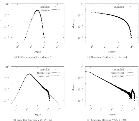
Figure 4共b兲 plots the sampled degree distribution for ␬ = 32,N= 216_{for dimensionm= 6. The corresponding plot for} a uniform hypersphere 关Fig. 4共a兲兴 is plotted alongside; the deviation from a Poisson distribution is clear.

In Fig. 5共b兲 the estimated fraction of the network occu-pied by the largest component is plotted against mean con-nectivity with increasing network size for dimension m= 6. Compared with the corresponding plot for a uniform

hyper-0 0.2 0.4 0.6 0.8 1

0 2 4 6 8

fraction

o

f

ne

tw

o

rk

si

ze

κ N= 28

N= 210

N= 212

N= 214

(a) Uniform hypersphere, dim = 6

0 0.2 0.4 0.6 0.8 1

0 2 4 6 8

fract

ion

of

n

et

w

ork

size

κ N= 28

N= 210

N= 212

N= 214

(b) Gaussian (Section V B), dim = 6

0 0.2 0.4 0.6 0.8 1

0 10 20 30 40

fraction

o

f

ne

tw

o

rk

si

ze

κ N= 28

N= 210

N= 212

N= 214

(c) Scale free (Section V C),β= 0.3

0 0.2 0.4 0.6 0.8 1

0 10 20 30 40

fract

ion

of

n

et

w

ork

size

κ N = 28

N = 210

N = 212

N = 214

[image:13.612.68.542.48.458.2]

(d) Scale free (Section V C),β= 0.6

sphere 关Fig. 5共a兲兴, where a phase transition can clearly be

seen, this supports our conjecture 共Sec. III F兲 that there should be no phase transition for a nonuniform GRGG and that the size of the largest component increases smoothly with increasing connectivity.

In Fig. 6共b兲 conditional arithmetic and harmonic mean path lengths are plotted against network size for dimension m= 6 alongside the corresponding plots for a uniform hyper-sphere of the same dimension关Fig.6共a兲兴, for mean

connec-tivity ␬= 12. As mentioned earlier, the mean scaling with network size is predicted reasonably accurately by the lower bounds as calculated in Eqs.共73兲and共74兲. In Figs.7共b兲and

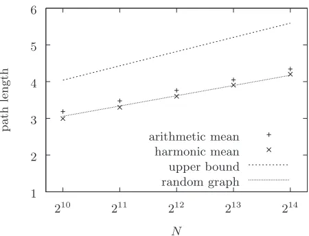
7共a兲corresponding path lengths are plotted for small world ensembles constructed according to the method described in Sec. IV, withc= 1. The plots labeled “random graph” show arithmetic mean path lengths for an Erdös-Rényi random graph with the same mean connectivity␬˜ as the correspond-ing small world ensemble; upper bounds are arithmetic mean path lengths for random graphs with mean connectivityNq

as in Eq. 共88兲. In this case the scaling of arithmetic mean

path length with network size appears to be reasonably well approximated by that of the corresponding random graph; there is, however, probably insufficient data to be certain.

C. Example 2: A scale free GRGG

Here we choose the underlying space to be the line seg-ment 共0 , 1兴 with standard metric d共x,y兲=兩x−y兩 and degree distributionXwith density:

p共x兲=共1 −␤兲x−␤ 共␤⬍1兲. 共112兲 Note that this density 共and hence the GRGG兲 is not uni-formly continuous. This is basically the situation covered in 关15兴 共Sec. III A兲, but note that scaling in the large network limit in that paper isnotthe same as ours; while we hold the mean degree␬fixed, there it is assumed thatrscales asN−1 共in particular we note that under their scheme mean node degree blows up withNfor ␤ⱖ1₂兲.

1 2 4 8

210 211 212 213 214

pa

thl

en

gt

h

N

arithmetic mean arithmetic mean lower bound harmonic mean harmonic mean lower bound

(a) Uniform hypersphere, dim = 6,κ= 12

1 2 4 8

210 211 212 213 214

pa

th

le

ng

th

N

arithmetic mean arithmetic mean lower bound harmonic mean harmonic mean lower bound

(b) Gaussian (Section V B), dim = 6,κ= 12

1 4 16 64 256

210 211 212 213 214

pa

thl

en

gt

h

N

arithmetic mean arithmetic mean lower bound harmonic mean

(c) Scale free (Section V C),β= 0.3,κ= 48

1 4 16 64 256

210 211 212 213 214

pa

th

le

ng

th

N

arithmetic mean arithmetic mean lower bound harmonic mean

[image:14.612.74.545.55.454.2]

(d) Scale free (Section V C),β= 0.6,κ= 48