Taylor's theorem for matrix functions with applications to condition number estimation

Contents lists available atScienceDirect

Linear

Algebra

and

its

Applications

www.elsevier.com/locate/laa

Taylor’s

theorem

for

matrix

functions

with

applications

to

condition

number

estimation

Edvin Deadman, SamuelD. Relton∗

SchoolofMathematics,TheUniversityofManchester,Manchester,M139PL,UK

a r t i c l e i n f o a bs t r a c t

Article history:

Received27April2015 Accepted6April2016 Availableonline18April2016 SubmittedbyV.Mehrmann

MSC:

15A12 15A16

Keywords:

Matrixfunction Taylorpolynomial Remainder Conditionnumber Pseudospectrum Fréchetderivative

We derive an explicit formula for the remainder term of a Taylor polynomial of a matrix function. This formula generalizes a known result for the remainderof theTaylor polynomialforananalytic functionofa complexscalar. We investigatesomeconsequencesofthisresult,whichculminate in new upper bounds for the level-1 and level-2 condition numbersofamatrixfunctionintermsofthepseudospectrum of the matrix. Numerical experiments show that, although theboundscanbe pessimistic,they canbecomputedmuch faster than the standard methods. This makes the upper boundsidealforaquickestimationoftheconditionnumber whilsta moreaccurate(andexpensive)methodcanbeused iffurtheraccuracyisrequired.Theyarealsoeasilyapplicable tomorecomplicatedmatrixfunctionsforwhichnospecialized conditionnumberestimatorsarecurrentlyavailable.

© 2016TheAuthors.PublishedbyElsevierInc.Thisisan openaccessarticleundertheCCBYlicense (http://creativecommons.org/licenses/by/4.0/).

✩ _{ThisworkwassupportedbyEuropeanResearchCouncilAdvancedGrantMATFUN(267526).}

* Correspondingauthor.

E-mailaddresses:[email protected](E. Deadman),[email protected]

(S.D. Relton).

http://dx.doi.org/10.1016/j.laa.2016.04.010

1. Introduction

Taylor’stheoremisastandardresultinelementarycalculus(seee.g.[17]).Iff :R→R isktimescontinuouslydifferentiableata∈R,thenthetheoremstatesthatthereexists

Rk :R→Rsuchthat

f(x) =

k

j=0

f(j)_(a)

j! (x−a)

j_+R k(x)

and Rk(x) = o(|x−a|k) as x → a. Depending on any additional assumptions on f,

variouspreciseformulaefortheremaindertermRk(x) areavailable.Forexample,iff is

k+ 1 timescontinuouslydifferentiableontheclosedintervalbetweenaandx,then

Rk(x) =

f(k+1)_(c) (k+ 1)! (x−a)

k+1 ₍₁₎

for some c between a and x. This is known as the Lagrange form of the remainder. Alternativeexpressions,suchastheCauchyform ortheintegralformfortheremainder arewellknown[17].

Taylor’stheoremgeneralizestoanalyticfunctionsinthecomplexplane:theremainder mustnow beexpressed intermsof acontourintegral.Iff(z) iscomplexanalyticinan opensubsetD ⊂Cofthecomplexplane,thekth-degreeTaylorpolynomialoff ata∈ D

satisfies

f(z) =

k

j=0

f(k)_(a)

k! (z−a)

j_+R k(z),

where

Rk(z) =

(z−a)k+1 2πi

Γ

f(w)dw

(w−a)k+1_(w−_z), (2)

andΓ isacircle,centredat a,suchthatΓ⊂ D.See[1,Chap. 5, Sec. 1.2]foraproof of thisresult.

The first goal of this paper is to generalize (2) to matrices, thereby providing an explicit expression for the remainder term for the kth-degree Taylor polynomial of a matrixfunction.Notethatitwillnotbe possibleto obtainanexpression similarto (1)

becauseits derivation relies on the mean valuetheorem which does nothave anexact analoguefor matrix-valued functions.Our second goal is to investigate applications of this result in bounding the derivatives and condition numbers of matrix functionsvia pseudospectra.

exposition). Mathias [15] also obtains a normwise truncation error bound for matrix function Taylorpolynomials whichform partof theSchur–Parlettalgorithm [4]. There are also a number of remainder theorems within the operator theory literature which can be appliedto matrix functions. However, to our knowledge, this paper represents the firsttimeanexplicit remainderterm(as opposedto abound) hasbeen specifically obtainedfortheTaylorpolynomialofamatrixfunction.

The remaining sections of this paper areorganized as follows. In section2 we state andprovetheremaindertermforthekth-degreeTaylorpolynomialofamatrixfunction. In section 3weinvestigate someapplications of thisresult bybounding the firstorder remaindertermusingpseudospectraltechniquesandrelatingittotheconditionnumber off(A).Insection4weextendtheseresultstothelevel-2conditionnumberofamatrix function,introducedin[13].Insection5weexaminethebehaviourofthepseudospectral boundsonsometestproblemsandshowthattheycanbecomputedefficiently.Finallyin section6wepresent ourconclusionsanddiscusssomepotentialextensionsofthiswork.

2. RemaindertermforTaylorpolynomials

The Taylorseries theorems foundinHigham’s monograph [11] primarilyinvolve ex-pandingf(A) aboutamultipleoftheidentitymatrixI:

f(A) =

∞

j=0

f(j)(α)

j! (A−αI)

j_.

OurstartingpointisthemoregeneralTaylorseriesexpansionintermsofFréchet deriva-tives, obtainedbyAl-MohyandHigham [2,Thm. 1]. Supposethatf hasapowerseries expansion∞_j=0ajxj withradius ofconvergencer >0 centeredattheorigin.The

inte-riorofthecircle|x|< rdefinesasimplyconnectedopensetD.Then,givenA,E∈Cn×n

withΛ(A),Λ(A+E)⊂ D(whereΛ(X) denotesthespectrumofthematrixX),Al-Mohy and Highamprovedthat

f(A+E) =

∞

j=0 1

j!D [j]

f (A, E), (3)

where

D[_fj](A, E) = d

j

dtj

t=0

f(A+tE). (4)

terms,D[1]_f (A,E),coincideswiththe“standard”FréchetderivativeLf(A,E).

Addition-ally,ifA andE commutethenwe haveD[_fj](A,E)=Ej_f(j)_(A),wheref(j) _denotesthe

jthderivativeofthescalarfunctionf(x).

Before writing down the remainder term obtained by truncating the Taylor series in(3), wefirstrecallthestandardresultthat,foranyinvertibleA andB,

A−1−B−1=A−1(B−A)B−1. (5)

Wewillalsoneedthefollowinglemma.

Lemma2.1. LetX(t)=A−tB,wheret isascalar. Then

dj

dtj

t=0

X(t)−1=j!A−1(BA−1)j.

Proof. Notethat

d dtX

−1_=−X−1_XX−1_,

whereX denotesthederivativeofX,andthat,sincehigherderivativesofX vanish,

dj dtjX

−1_{= (−1)}j_j!X−1_(XX−1₎j_.

Theresultthen followsbysubstitutingX =A−tB andsettingt= 0. 2

Furthermore, we note that by the Cauchy–Hadamard theorem any power series in thecomplexplaneconvergingtoafunctionf mustconverge onacirculardomain with radiusofconvergencer(whichcanbeinfinite).Inthefollowingresults,forthepurpose ofmaximizinggenerality,wesaythatf hasapowerseriesexpansionwhichconvergeson asimplyconnectedopensetD.ClearlyDmustbeasubsetofthiscirculardomain,but neednotbe circularitself.Thereasonforthisdistinctionisthatthe-pseudospectraof

A,used insection3,giveriseto setsofdifferingshape.

Wenowstateandprovethemainresultofthispaper,whichgivesanexplicitformof theremaindertermwhentruncating(3).

Theorem 2.2.Let f have apower series expansionabout theoriginwith radiusof

con-vergence r and let D ⊂ C be a simply connected open set within thecircle of radius r centeredat0.LetA,E∈Cn×n besuchthat Λ(A),Λ(A+E)⊂ D.Thenforanyk∈N

f(A+E) =Tk(A, E) +Rk(A, E),

Tk(A, E) = k

j=0 1

j!D [j]

f (A, E), (6)

Rk(A, E) =

1 2πi

Γ

f(z)(zI−A−E)−1[E(zI−A)−1]k+1dz, (7)

and Γisaclosed contour inD enclosingΛ(A)and Λ(A+E).

Proof. Theresultisprovedbyinductiononk.For thecasek= 0 wehavef(A+E)=

f(A)+R0(A,E).Then

R0(A, E) =f(A+E)−f(A)

= 1 2πi

Γ

f(z)[(zI−A−E)−1−(zI−A)−1]dz,

using theCauchyintegraldefinitionofamatrixfunction.Itfollows from(5)that

R0(A, E) = 1 2πi

Γ

f(z)(zI−A−E)−1E(zI−A)−1dz.

Fortheinductivestep,weassumethatf(A+E)=Tk(A,E)+Rk(A,E).Theremainder

forthe(k+ 1)st degreeTaylorpolynomialisgivenby

Rk+1(A, E) =f(A+E)−Tk+1(A, E)

=f(A+E)−Tk(A, E)−

1 (k+ 1)!D

[k+1]

f (A, E)

=Rk(A, E)−

1 (k+ 1)!

dk+1 dtk+1

t=0

f(A+tE).

Substituting the inductive hypothesis for Rk(A,E) and the Cauchy integral form for

f(A+tE),assumingthattissufficientlysmall, gives

Rk+1(A, E) = 1 2πi

Γ

f(z)(zI−A−E)−1[E(zI−A)−1]k+1dz

− 1

2πi(k+ 1)!

dk+1 dtk+1

Γ

f(z)(zI−A−tE)−1dz.

Rk+1(A, E) =

1 2πi

Γ

f(z)(zI−A−E)−1[E(zI−A)−1]k+1

−(zI−A)−1[E(zI−A)−1]k+1dz

= 1 2πi

Γ

f(z)(zI−A−E)−1[E(zI−A)−1]k+2dz,

where(5)hasbeen usedoncemore.Thiscompletestheproof. 2

WeendthissectionbybrieflydescribinghowTheorem 2.2 alsoallowsusto obtaina remaindertermforPadéapproximants(thiswasfirstdoneinthescalarcasebyElliot[5]). Suppose that we approximate f(z) using a rational function pm(z)/qn(z), where

pm(z) and qn(z) are polynomials of degree m and n respectively. The Padé

approx-imant is the unique choice (up to scalar multiples) of pm(z) and qn(z) such that

f(z)−pm(z)/qn(z)=O(zm+n+1).Therefore,usingthesamerationalfunctionto

approx-imatethecorrespondingmatrixfunction,wehaveqn(X)f(X)−pm(X)=O(Xm+n+1).

Weintroducethetruncation errortermSm,n(X) tothePadé approximantsuchthat

f(X) =qn(X)−1pm(X) +Sm,n(X).

Then,byrearrangingtheabove,

qn(X)f(X) =pm(X) +qn(X)Sm,n(X).

Thetermqn(X)Sm,n(X) isthentheremaindertermifweconsiderpm(X) tobeapower

series expansion of qn(X)f(X) when we set A = 0 and E = X. The remainder has

degreeatleastm+nand so,byapplying(7)with k=m+n, weobtain

Sm,n(X) =

qn(X)−1Xm+n+1

2πi

Γ

qn(z)f(z)(zI−X)−1

zm+n+1 dz,

wheretheclosedcontourΓ enclosesΛ(X) andtheorigin.

3. Applicationto conditionnumbers andpseudospectra

InthissectionweuseTheorem 2.2tostudythebehaviouroftheconditionnumberof amatrixfunction, whichmeasures thesensitivity of f(A) tosmall perturbationsinA. The resultsin this section are applicable for any induced matrix norm. Our approach requires borrowing a number of techniques from the analysis of pseudospectra. Recall thatthe-pseudospectrumofamatrixX istheset

Λ(X) =

z∈C:(zI−X)−1 ≥−1 . (8)

Lemma 3.1. Let f andD satisfy the criteria of Theorem 2.2. Furthermore let >0be such that Λ(A)⊂ D and Λ(A+E)⊂ D,and take Γ˜⊂ D tobe aclosed contour that

encloses both Λ(A)andΛ(A+E).Then theremainderterm Rk(A,E) isboundedby

Rk(A, E) ≤

Ek+1_L˜

2πk+2 max

z∈Γ˜

|f(z)|, (9)

whereL˜ isthelengthofΓ˜.Inparticular,whenacircularcontourcenteredat0isused,

Rk(A, E) ≤

Ek+1_ρ˜

k+2 _θ∈max_[0,2π]|f( ˜ρe

iθ_{)|, (10)}

where ρ˜= max{|z|:z∈Λ(A+E)∩Λ(A)}is theradius ofthecircle.

(NotethattildesonL˜,Γ˜,andρ˜ areusedbecause,forthis resultonly,thecontour

needs to enclose Λ(A+E) in addition to Λ(A). For subsequent results, the contour

need onlyencloseΛ(A) andthetildes aredropped.)

Proof. Theproofisanalogousto thatofthebound

f(A) ≤ L˜ 2πmaxz∈Γ˜

|f(z)|,

obtained by Trefethen and Embree [19, Ch. 14]. We bound the norm of Rk(A,E) by

notingthat

Rk(A, E) ≤

Ek+1 2π

˜ Γ

|f(z)|(zI−A−E)−1(zI−A)−1k+1.

On Γ˜ we have(zI−A−E)−1≤−1 and(zI−A)−1≤−1. Thefirstpartof the

lemmafollowsimmediately.Forthesecondpart,takeΓ˜tobeacirclewithcenter0and

radius ρ˜= max{|z|:z∈Λ(A+E)∩Λ(A)}. 2

We can also use this result to bound the absolute condition number of a matrix function. Recallthattheabsolute conditionnumbermeasures thefirstordersensitivity of f(A) tosmallperturbationsinA andisgivenby[11,Chap. 3]

condabs(f, A) := lim

τ→0_Esup_≤τ

f(A+E)−f(A)

τ

= max

E≤1Lf(A, E). (11)

Corollary 3.2.Let f and D satisfy the criteria of Theorem 2.2. Let > 0 be such that Λ(A) ⊂ D, and let Γ ⊂ D be a closed contour of length L that encloses the

-pseudospectrum.Then

condabs(f, A)≤ L 2π2max_z∈Γ

|f(z)|. (12)

Inparticular, whenacircularcontour centeredat0isused,

condabs(f, A)≤ ρ

2_θ∈max_[0,2π]|f(ρe

iθ_{)|, (13)}

whereρ= max{|z|:z∈Λ(A)}isthepseudospectralradiusof A.

Proof. Set k= 0 in (9). ConsiderE=α < so that,by anequivalent definition of

the-pseudospectrum,wehaveΛ(A+E)⊂Λ(A).Then,sinceR0(A,E)=Lf(A,E)+

o(E),wehave

Lf(A, E) +o(α) ≤

αL

2π2max_z∈Γ|f(z)|.

Wedividebyαandtakethesupremumover allE suchthatE≤αtoobtain

sup

E≤α

Lf(A, E/α) +o(α)/α ≤

L

2π2max_z∈Γ

|f(z)|.

Theproofof(12)iscompletedbytakingthelimitα→0 andrecallingthattheabsolute condition number of a matrix function is given by the operator norm of the Fréchet derivative(11).

The proof of (13) is essentially the same, except that (10) is taken as the starting pointratherthan(9).

Notethatan alternativeproof ofthecorollary canbe obtainedbystartingwith the integralrepresentation oftheFréchetderivative

Lf(A, E) =

1 2πi

Γ

f(z)(zI−A)−1E(zI−A)−1dz,

andboundingitaboveusingthetechniquesfrom theproofofLemma 3.1. 2

Lemma 3.3(Reddy, Schmid, and Henningson).Let W(A) be the numerical range of A and Δδ be acloseddisk of radiusδ.Thenforall>0

Λ(A)⊂W(A) + Δ,

wheresetadditionisdefinedcomponentwise;thatisS1+S2={s1+s2:s1∈S1, s2∈S2}.

Proof. SeeReddy, Schmid,andHenningson[16, Thm. 2.1]. 2

Since the numerical radius, r(A) := sup_z∈W(A)|z|, is equal to A2 we know that the -pseudospectral radius is no larger than A2+. Thus we obtain the following corollary.

Corollary 3.4.Letf,D,and>0satisfythecriteria ofCorollary 3.2andsuppose that

A2+< r,theradiusof convergenceforthepowerseriesexpansionof f.Then

condabs(f, A)≤

A2+ 2 _|z|=max_A

2+|

f(z)|. (14)

Proof. Thecircle of radiusA2+around theoriginencloses Λ(A) andis of length

2π(A2+).Usingthis contourin(13)givesthedesiredresult. 2

Onepotentialapplicationofthisresultisinthedesignandanalysisofalgorithmsfor computing matrixfunctions. Manysuch algorithms workbyrescalingA to be ofsmall norm, applying the function to this scaled matrix (via a Padé approximant or Taylor series),andthenundoingtheeffectofthescaling.Thiscorollarymayallowustobetter understand the numerical effect of applying the matrix function to the scaled matrix, sincesuchanalysisis typicallydoneonlyinexactarithmetic.

WeendthissectionbybrieflymentioningarelatedtheoremduetoLui[14,Thm. 3.1], concerning the relationshipbetween thepseudospectra of Aand f(A). Thetheorem is restatedhereinournotation.RecallthatRk(A,E) wasdefinedinTheorem 2.2andthat

R0(A,E)=Lf(A,E)+o(E).

Lemma 3.5(Lui). Let,f,andΓ satisfy theconditions of Corollary 3.2.Furthermore

let f(Λ(A))= {f(z) :z ∈ Λ(A)}and M = maxE≤R0(A,E). Then f(Λ(A))⊂

ΛM(f(A)).

Proof. IfzisaneigenvalueofA+E withE≤(so thatz∈Λ(A)),thenf(z) isan

eigenvalueoff(A+E)=f(A)+R0(A,E) andR0(A,E)≤M. 2

Thisresultshowsthat,tofirstorderin,the-pseudospectrumofAisrelatedtothe

4. Applicationto higherorderconditionnumbers

HighamandRelton[13] introducethelevel-qconditionnumberformatrixfunctions, whichisdefinedrecursivelyby

cond(_absq)(f, A) := lim

α→0_Zsup_≤α

|cond(_absq−1)(f, A+Z)−cond(_absq−1)(f, A)|

α , (15)

wherecond(1)_abs(f,A):= condabs(f,A).Insection3wefocusedonthefirstorderremainder term, R0(A,E), and results concerning the condition number condabs(f,A) but – by choosingk >0 in Lemma 3.1–wecanattempttoextendresultssuchas Corollary 3.2

tothese higherorder conditionnumbers.

Beforeproceeding,we must firstinvestigate therelationshipbetween theD[_fj](A,E) defined in(4) and higher order Fréchet derivatives.Recall thatD_f[j](A,E) isa special caseofthejthorderFréchetderivativeinwhichtheperturbationineachdirectionisE. In[13]adefinitionofthejthorderFréchetderivative,assumingitiscontinuousinA,is givenintermsofthemixedpartialderivative:

L(_fj)(A, E1, . . . , Ej) =

∂ ∂s1· · ·

∂ ∂sj

(s1,...,sj)=0

f(A+s1E1+· · ·+sjEj). (16)

Thefollowingtheorem expressesthisjthorder Fréchetderivativeintermsofacontour integral.

Theorem4.1. Letf be j timesFréchetdifferentiablesuchthat thejthFréchetderivative

iscontinuousatA,andletΓ beaclosed contourenclosingΛ(A)suchthatf isanalytic insideandonΓ.Then,thejthorderFréchetderivativeof amatrixfunctionf(A)inthe directionsE1,. . . ,Ej isgivenby

L(_fj)(A, E1, . . . , Ej) =

1 2πi

Γ

f(z)(zI−A)−1

σ∈Sj

k

i=1

Eσ(i)(zI−A)−1dz, (17)

whereSjisthesetofpermutationsof{1,2,. . . ,k}.InparticularthederivativeD[_fj](A,E)

isgivenby

D_f[j](A, E) = j! 2πi

Γ

f(z)(zI−A)−1[E(zI−A)−1]j+1dz. (18)

Proof. For any choiceof si (in someneighbourhoodof 0) and Ei,we canwrite f(A+

s1E1+· · ·+sjEj) asaCauchyintegralbyusingthestandardCauchyintegraldefinition

L(_fj)(A, E1, . . . , Ej) =

∂ ∂s1· · ·

∂ ∂sj

(s1,...,sj)=0

˜ Γ

f(z)(zI−(A+s1E1+· · ·+sjEj))−1dz.

Using theLeibnizintegralrule,thedifferentialoperator

∂ ∂s1· · ·

∂ ∂sj

(s1,...,sj)=0

canbebroughtinsidetheintegralsign.Therequiredintegrandisthenobtainedbyusing theidentity

d dxU

−1_=−U−1dU

dxU −1_.

Theresult(17)follows bythenrestrictingthecontourtotheclosed curveΓ containing Λ(A).Thesecondpartofthetheorem,(18),followsbysettingE1=· · ·=Ej. 2

Theorem 4.1 shows that, to firstorder, thekth remainder term intheTaylor series issimplythe(k+ 1)st derivative,as wemightexpect.Specifically,comparing (18)with

(7) wefind

Rk(A, E) =

1 (k+ 1)!D

[k+1]

f (A, E) +o(E k+2_).

In addition, Theorem 4.1 allows us to prove the following theorem,which uses the pseudospectrumofAto boundthenormofthejthorder Fréchetderivative.

Theorem 4.2.Let f satisfy the criteria of Theorem 4.1 and let Γ be a closed contour

enclosing Λ(A) such that f is analytic inside and on Γ. Then the jth order Fréchet

derivative can bebounded by

L(_fj)(A, E1, . . . , Ej) ≤

j!L

2πj+1

max

z∈Γ|

f(z)|

j

i=1

Ei, (19)

where L isthelengthof Γ.

Proof. In (17) use the contour Γ, take norms, and note that (zI −A)−1 ≤ −1

on Γ. 2

any interest. Instead we restrict ourselves to the case q = 2 and the level-2 condition number.

Lemma4.3.Letf satisfythecriteriaofTheorem 4.1andletΓaclosedcontourenclosing

Λ(A)suchthat f isanalytic inside andonΓ.Thelevel-2conditionnumber isbounded

by

cond(2)_abs(f, A)≤ L

π3max_z∈Γ|f(z)|.

Whenacircularcontour centeredat0isused,

cond(2)_abs(f, A)≤ 2ρ

3 _θ∈max_[0,2π]|f(ρe

iθ_)|,

whereρ,thepseudospectralradius, istheradiusof thecircle.

Proof. Higham and Relton [13, Sec. 5] give an upper bound for the level-2 absolute

conditionnumberintermsofthenormofthesecondFréchetderivative

cond(2)_abs(f, A)≤ max

E1=1

max

E2=1

L(2)_f (A, E1, E2). (20)

Substitutingtheboundfrom(19)into(20)givestherequiredresults. 2

5. Numericalexperiments

In this section we show how our pseudospectral bounds on the condition number,

(12) and (13), can be used to estimate the condition number of matrix functions in practice.Wealsofindthattheyarecheaperthanalternativeapproachesand,therefore, onemight use thepseudospectral bound as aquick estimate of thecondition number. If this estimate is unsatisfactorily large we can use existing methods to estimate it moreaccurately.Theterm“unsatisfactorilylarge”canbemadepreciseinthefollowing manner:manyapplicationsonlyrequirethefirstfewdigitsoftheresulttobecorrectso thatarelativeerrorof,forexample,1e-4isperfectlyacceptable.Whenusingabackward stable algorithm the relative error is approximately bounded above by the condition numbermultipliedbytheunitroundoff(u= 2−53_{inIEEEdoubleprecisionarithmetic).} Throughoutthissection, tocomputeourboundontheconditionnumber,wewill be using(12)

condabs(f, A)≤ L

2π2max_z∈Γ|f(z)|,

whereΓisaclosedcontouroflengthLthatenclosesthepseudospectrumofAandlies

condrel(f, A) = condabs(f, A) A f(A).

Combining these two results allows us to bound the relative condition number from above.ThisboundwillbecheaptocomputeprovidedthatthecostofcomputingLand

maxz∈Γ|f(z)|is sufficientlysmall.

Inordertousethisboundinpracticewemustchoosewhichmatrixnormtoconsider, thevalueof ,andthecontourΓ. WewillusetheFrobeniusnorm since,inthisnorm,

there isanexplicitformulafortheconditionnumberwhichcanbecomputedusing[11, Alg. 3.17]. However, the pseudospectrum is not defined in the Frobenius norm, since it requires the use of an induced norm. To resolve this, one can easily show that the absolute condition number in the Frobenius norm is bounded above by √n times the conditionnumberinthe2-norm,where nisthesize ofthematrix.Hencewehave

condrel(f, A, · F)≤

√

ncondabs(f, A, · 2)

AF

f(A)F

.

Theright-handsideofthisequationiswhatwewillcompute,wherethecondabs(·) term is boundedaboveby(12).

It remainsto chooseand Γ.Lookingat (12)wesee that,heuristically,inorder to

minimizetheupperboundwewouldliketobereasonablyfarfrom0.Someofourtest functions will have power series thatare convergent in acircle of radius 1 around the point z = 0; for these caseswe chooseΓ to be acircle centered at 0 with radius 0.99

and find thelargest such thatthe-pseudospectral radiuslies insidethis circle. This is computedusingthenonlinearoptimizationroutinefminbndinMATLAB.Whenour function hasapowerseries with aninfiniteradius ofconvergence we choose= 1 and take Γ to be acircle centeredat the meanof theeigenvalues of A(γ = _n1

λi)with

radiusequaltothe-pseudospectralradiusofA−γI.Finally,tofindmax|f(z)|onthese contours,weagainusethenonlinearoptimizationroutinefminbndinMATLAB.Weuse

psapsrbyGuglielmiandOverton[7]tocomputethe-pseudospectralradiithroughout. Wewillcompareourpseudospectralmethoddescribedabove(hereafterreferredtoas

condpseudo)intheFrobeniusnormagainsttwoalternativemethodsforcomputingthe condition number: funm_condest_fro from the Matrix Function Toolbox [10] and an “exact” methoddetailed byHigham [11, Alg. 3.17], which we referto as condold and

condexact, respectively.

The method condold uses finite difference approximations to the derivatives of the matrixfunctionandhasO(n3_{) cost.Meanwhilecondexactexpressesthecondition} num-berasthe2-normofamatrixKf(A)∈Cn

2_×n2

,calledtheKroneckerformofthematrix function, which must be computed explicitly with cost O(n5). Therefore condexactis impractical forallbutthesmallestproblems.

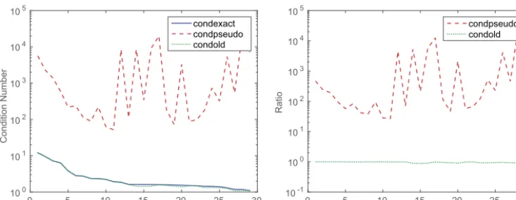
Fig. 1.Conditionnumberestimates/boundsforthematrixfunctioncorrespondingtof(x)= log(1+x) in theFrobeniusnormover29 testmatrices.Wehavecondoldandcondexactoverlappingalmostentirely.Left:

Theconditionnumberestimates/bounds.Right:Theratiosofcondpseudoandcondoldtocondexact.

Wecomparethethreedifferentalgorithmsonfourmatrixfunctionscorresponding to thescalarfunctionslog(1+x),(1+x)1/15_{,exp(x),andcos(x).Thefirsttwoofthesehavea} powerseriesrepresentationwhichisconvergentfor|x|<1,whilstthelatterhaveglobally convergent power series. The matrix functions are computed using logm and expm in MATLAB,alongwithcosmfrom[3],andpowerm_fre_newbyHigham and Lin [12].

For each function we use 29 test matrices (of size n = 10) from the Matrix Com-putation Toolbox [9] and plot both the computed condition numbers and the ratio of

condpseudoand condoldto condexact.For thefirsttwo functions,where we needall eigenvalues to lie within the region of convergence, we transform each matrix to have eigenvalues centered at 0 with A2 = 1 so that all eigenvalues lie within the unit disk.

InFig. 1 we see the condition numberas computed by the three methods,for each of the 29 test matrices, using the functionf(x)= log(1+x). The resultsare ordered by decreasing condition number as computed by condexact. We can immediately see thatcondpseudoisindeedanupperboundandisusually2–4ordersofmagnitudelarger thantheexactconditionnumber.Meanwhilecondoldisgenerallyaverygoodestimate oftheconditionnumber.

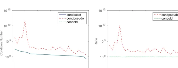
Next inFig. 2 we compare the condition numberswhen using the function f(x) = (1+x)1/15_{.Inthiscaseweseeverysimilarbehaviourtothepreviousfunction:condold} andcondexactarealmostidenticalwhilstcondpseudoprovidesanupperboundthatis generally2–4ordersofmagnitude largerthanthetrueconditionnumber.

Fig. 3showstheresultswhenusingf(x)= exp(x).Inthiscasecondpseudoperforms slightlybetterthanpreviouslybeing only1–3ordersofmagnitudeabovecondexacton mosttestproblems.

eigen-Fig. 2.Conditionnumberestimates/boundsforthematrixfunctioncorrespondingtof(x)= (1+x)1/15in theFrobeniusnormover29 testmatrices.Wehavecondoldandcondexactoverlappingalmostentirely.Left:

Theconditionnumberestimates/bounds.Right:Theratiosofcondpseudoandcondoldtocondexact.

Fig. 3.Conditionnumberestimates/boundsforthematrixfunctioncorrespondingtof(x)= exp(x) inthe Frobeniusnormover29 test matrices.Wehavecondoldandcondexactoverlappingalmostentirely.Left:

Theconditionnumberestimates/bounds.Right:Theratiosofcondpseudoandcondoldtocondexact.

Fig. 4.Conditionnumberestimates/boundsforthematrixfunctioncorrespondingtof(x)= cos(x) inthe Frobeniusnormover29 test matrices.Wehavecondoldandcondexactoverlappingalmostentirely.Left:

valuesextendingfar intothecomplexplane:as thecosinefunctiongrowsexponentially inthedirectionoftheimaginaryaxis|cos(z)|is extremelylargeonthechosencontour. Each ofthese four casesshowsthatcondpseudoprovides areliableupperbound on the condition number and is generally just a few orders of magnitude above the true value. We also note that, since condpseudo needs only the scalar function f(x) and doesnot needto compute thederivativesof amatrixfunction, viafinite differences or otherwise,itcaneasilybeappliedtoverycomplicatedmatrixfunctionssuchascos(√A) (forwhichnospeciallydesignedalgorithmsexist)withnomodification.Inthisparticular casewewouldapply ouralgorithm tothefunction

f(A) =

∞

k=0

(−1)kAk

(2k!) ,

which isanalytic and equivalent to cos(√A) away from theorigin, regardless of which branch of the square root function is selected. Matrix functions such as this can arise infiniteelementsemidiscretizationofthewaveequation.Forexample,thesecond order differentialequation

y(t) +Ay(t) =g(t), y(0) =y0, y(0) =y0,

hasthesolution

y(t) = cos(√At)y0+ ( √

A)−1sin(√At)y₀ +

t

0

(√A)−1sin√A(t−s)g(s)ds,

where√Adenotes anysquare rootof A[6,p. 124], [18];see also[11, Prob. 4.1]forthe caseg(t)= 0.

Our next experiment compares the speed of estimating the condition number as the size of the matrix grows. Here we focus on the function f(x) = (1+x)t _for

t = 1/5,1/15,1/52 and for n between 10 and 1000. For each value of n we take A

to be amatrix with elements normally distributed with zero mean and unit variance, scaledtohaveunitnorm.SincecondexactisanO(n5_{) algorithmitbecomesincreasing} impractical as n grows: instead we will compare condpseudo against condold and a differentalgorithm,condhili.Thislatteralgorithm,designedbyHighamand Lin[12], estimates thecondition number of matrixpowers ina similar manner to condold but actuallycomputesthederivativesof thematrixfunction,as opposedtousing finite dif-ferenceapproximations. Thealgorithmisdesignedto estimatetheconditionnumberin the 1-norm but has similar computational complexity to condold which works in the Frobeniusnorm.ThisexperimentwasrunonalaptopwithanInteldual-corei7processor usingMATLABR2014b.

Fig. 5. Runtimein secondsandresultingspeedup whencomputingthematrixfunction correspondingto

f(x)= (1+x)t_{fort= 1/5,1/15,1/52 usingcondpseudo,condold,andcondhiliasnvariesbetween10 and}

1000.Thex-axisshowsn,thesizeofthetestmatrix,whilstthey-axisdenotestheruntimeandspeedup, respectively.Left:Runtimeinsecondswhenrunningeachalgorithm.Right:Speedupwhenusingcondpseudo comparedtocondoldandcondhili.

of t whilst the right-hand plot shows the speedup when using condpseudo relative to theothermethods.Thex-axis showsn,thesizeofthematrices,whilstthey-axisshows theruntimeinseconds(left-handplot)andthespeedupobtained(right-handplot).We see that condpseudo is much cheaper than the alternatives for fairly small matrices and appearsto settle at around1.5 timesfaster than condoldand 2times fasterthan

condhili,respectively, onthis machine. This wouldsuggest thatusing condpseudois beneficial forapplications wherelow-accuracy solutionsare requiredandisparticularly goodinsituationswhere lotsofsmallmatrixfunctionsneedtobe computed.

6. Conclusions

Themainresultsinthispaperareasfollows.Wehaveobtainedanexplicitexpression fortheremaindertermofamatrixfunctionTaylorpolynomial(Theorem 2.2).Combining this with use of the -pseudospectrum of A leads to upper bounds on the condition numbers of f(A). Our numerical experiments demonstrated that our bounds can be used for practical computations: they provide a cheap upper bound on the condition number which is often onlya few orders of magnitude too large. This meansthat our bounds could beused as aquickestimateof theconditionnumberand ifthis estimate is too large,forinstance if theestimatesuggeststhatan insufficientnumberofcorrect significant figuresmightbe obtainedincomputing f(A),then existingmethodscanbe used toobtaintheconditionnumbermoreaccurately.

Anotherbenefitofourapproachisthatitcaneasilybeappliedtoboundthecondition numberofcomplicatedmatrixfunctionssuchascos(√A) withoutmodification,asthere are currentlynospecializedmethodsforcomputingsuchquantities.

thebehaviourof existingalgorithmsto computematrixfunctions(see thediscussion of

Corollary 3.4).This willbethesubjectoffuturework.

Acknowledgements

WeareverygratefultoNickHighamfornumeroushelpfulcommentsonearlierdrafts of this work and to the referee who helped to significantly increase the quality of the manuscript.

References

[1]LarsV.Ahlfors,ComplexAnalysis,thirdedition,McGraw-Hill,NewYork,ISBN 978-0-0700-0657-7, 1979.

[2] AwadH.Al-Mohy,NicholasJ.Higham,ThecomplexstepapproximationtotheFréchetderivativeof amatrixfunction,Numer.Algorithms53 (1)(2010)133–148, http://dx.doi.org/10.1007/s11075-009-9323-y.

[3] AwadH.Al-Mohy,NicholasJ.Higham,SamuelD.Relton,Newalgorithmsforcomputingthematrix sine and cosine separately or simultaneously, SIAM J. Sci. Comput. 37 (1) (2015) A456–A487,

http://dx.doi.org/10.1137/140973979.

[4] PhilipI.Davies, NicholasJ.Higham,ASchur–Parlettalgorithmforcomputingmatrixfunctions, SIAMJ.MatrixAnal.Appl.25 (2)(2003)464–485,http://dx.doi.org/10.1137/S0895479802410815. [5]David Elliott,Truncation errors inPadé approximationsto certainfunctions: an alternative

ap-proach,Math.Comp.(ISSN 0025-5718) 21 (99)(1967)398–406.

[6]F.R.Gantmacher,TheTheoryofMatrices,vol.1,Chelsea,NewYork,ISBN 0-8284-0131-4,1959.

[7]NicolaGuglielmi,MichaelL.Overton,Fastalgorithmsfortheapproximationofthepseudospectral radiusofamatrix,SIAMJ.MatrixAnal.Appl.32 (4)(2011)1166–1192.

[8]KurtHensel,ÜberPotenzreihenvonMatrizen,J.ReineAngew.Math.155 (42)(1926)100–110.

[9] Nicholas J. Higham, The Matrix Computation Toolbox, http://www.maths.manchester.ac.uk/ ~higham/mctoolbox.

[10] NicholasJ.Higham,TheMatrixFunctionToolbox,http://www.maths.manchester.ac.uk/~higham/ mftoolbox.

[11]NicholasJ.Higham, FunctionsofMatrices: TheoryandComputation,Societyfor Industrialand AppliedMathematics,Philadelphia,PA,USA,ISBN 978-0-898716-46-7,2008.

[12] Nicholas J. Higham, Lijing Lin: An improved Schur–Padé algorithm for fractional powers of a matrix and their Fréchet derivatives, SIAM J. Matrix Anal. Appl. 34 (3) (2013) 1341–1360,

http://dx.doi.org/10.1137/130906118.

[13] Nicholas J. Higham, Samuel D. Relton, Higher order Fréchet derivatives of matrix functions and the level-2 condition number, SIAM J. Matrix Anal. Appl. 35 (3) (2014) 1019–1037,

http://dx.doi.org/10.1137/130945259.

[14]S.-H.Lui,Apseudospectralmappingtheorem,Math.Comp.72 (244)(2003)1841–1854.

[15]RoyMathias,Approximationofmatrix-valuedfunctions,SIAMJ.MatrixAnal.Appl.14 (4)(1993) 1061–1063.

[16] S.C.Reddy,P.J.Schmid,D.S.Henningson,PseudospectraoftheOrr–Sommerfeldoperator,SIAM J.Appl.Math.53(1993)15–47,http://dx.doi.org/10.1137/0153002.

[17]Walter Rudin, Real and Complex Analysis, third edition, McGraw-Hill, New York, ISBN 0070542341,1986.

[18] StevenM.Serbin,Rationalapproximationsoftrigonometricmatriceswithapplicationto second-ordersystemsofdifferentialequations,Appl.Math.Comput.5 (1)(1979)75–92,http://dx.doi.org/ 10.1016/0096-3003(79)90011-0.

[19]LloydNicholasTrefethen,MarkEmbree,SpectraandPseudospectra:TheBehaviorofNonnormal MatricesandOperators,PrincetonUniversityPress,2005.

[20] H.W.Turnbull,Amatrix formof Taylor’stheorem,Proc.Edinb.Math.Soc.(2)2 (1930)33–54,

http://dx.doi.org/10.1017/S0013091500007537.