The Shallow-Marine Architecture Knowledge Store: a database for the characterization of shallow-marine and paralic depositional systems

This is a repository copy of The Shallow-Marine Architecture Knowledge Store: a database

for the characterization of shallow-marine and paralic depositional systems.

White Rose Research Online URL for this paper:

http://eprints.whiterose.ac.uk/97154/

Version: Accepted Version

Article:

Colombera, L, Mountney, NP, Hodgson, DM et al. (1 more author) (2016) The

Shallow-Marine Architecture Knowledge Store: a database for the characterization of

shallow-marine and paralic depositional systems. Marine and Petroleum Geology, 75. pp.

83-99. ISSN 0264-8172

https://doi.org/10.1016/j.marpetgeo.2016.03.027

© 2016, Elsevier. Licensed under the Creative Commons

Attribution-NonCommercial-NoDerivatives 4.0 International

http://creativecommons.org/licenses/by-nc-nd/4.0/

[email protected] https://eprints.whiterose.ac.uk/

Reuse

Unless indicated otherwise, fulltext items are protected by copyright with all rights reserved. The copyright exception in section 29 of the Copyright, Designs and Patents Act 1988 allows the making of a single copy solely for the purpose of non-commercial research or private study within the limits of fair dealing. The publisher or other rights-holder may allow further reproduction and re-use of this version - refer to the White Rose Research Online record for this item. Where records identify the publisher as the copyright holder, users can verify any specific terms of use on the publisher’s website.

Takedown

If you consider content in White Rose Research Online to be in breach of UK law, please notify us by

1

The Shallow-Marine Architecture Knowledge Store: a database for the

characterization of shallow-marine and paralic depositional systems

Luca Colombera, Nigel P. Mountney, David M. Hodgson, William D. McCaffrey

Shallow-Marine Research Group, School of Earth and Environment, University of Leeds, LS2 9JT, Leeds, UK

Abstract

The Shallow-Marine Architecture Knowledge Store (SMAKS) is a relational database devised for the storage of hard and soft data on the sedimentary architecture of ancient shallow-marine and paralic siliciclastic successions, and on the geomorphological

organization of corresponding modern environments. The database allows incorporation of data from the published literature, which are uploaded to a common standard to ensure consistency in data definition. The database incorporates data on geological entities of varied nature and scale (i.e., surfaces, depositional tracts, architectural elements, sequence stratigraphic units, facies units, geomorphic elements), including attributes that characterize their type, geometry, spatial relations, hierarchical relations, and temporal significance. Furthermore, geological entities are assigned to depositional systems, or to parts thereof, that can be classified on multiple parameters (e.g., shelf width, delta catchment area) tied to metadata (e.g., data types, data sources).

The SMAKS permits the quantitative characterization of modern and ancient shallow-marine and paralic clastic depositional systems. It aims to serves as a repository of analogue information for hydrocarbon-bearing successions, and as a research tool, applicable to aid the development of facies models or to assess the sensitivity of depositional systems to particular controlling factors, for example.

To demonstrate the wide applicability of the database in fields of both fundamental and applied research, example database output is presented that (i) includes data from wave-, tide-, and fluvial-dominated shallow seas and sedimentary successions, and (ii) covers a wide depositional spectrum, from backshore to shelf-edge settings. The examples include information onthe facies organization of different types of paralic sub-environments, on the hierarchical arrangement of architectural elements that form deltaic constructional units in Quaternary deltas, on the morphometry of modern and Quaternary tidal sand ridges, and on the geometry of parasequence-scale nearshore sandstone beltsfrom the Upper Cretaceous of the Western Interior Seaway in Utah (USA).

2

Introduction

Improvement in subsurface prediction of shallow-marine and paralic siliciclastic hydrocarbon reservoirs is typically attempted through the characterization of ancient and modern

depositional systems that represent potential reservoir analogues. Analogue data are applied in scenarios of reservoir exploration, development and production: (i) to predict the potential occurrence and size of stratigraphic traps (cf. Posamentier 2002); (ii) to predict the seismic resolvability of sedimentary bodies (cf. Tomasso et al. 2009); (iii) to erect conceptual reservoir models (cf. Nielsen & Johannessen 2001); (iv) to guide well-to-well correlations of sedimentary units (cf. Wood 2004); (v) to condition static reservoir models (cf. Howell et al. 2008; 2014). Ancient and modern analogues are generally characterized through a number of approaches and at multiple scales of observation (e.g., sedimentary facies and

architectural-element analysis of ancient outcrop successions, mapping key stratal surfaces at outcrop or in seismic data to erect a sequence stratigraphic framework, analysis of aerial photographs or satellite imagery of modern environments).

Databases may be constructed to assist the application of analogue data to subsurface workflows in industry practice. However, such databases tend to offer only a partial

characterization of the sedimentary architecture of the geological analogues, and are limited to quantitative descriptions of the geometry of sedimentary units. Furthermore, they do not generally capture sedimentological data on hierarchical and spatial relationships, stacking patterns, facies proportions, and stratigraphic distribution of genetic units at multiple scales. The amount of data derived from studies of ancient and modern analogues and made available in the peer-reviewed scientific literature is constantly increasing. However, making these data accessible in meaningful and usable formats is not trivial, particularly given the varied types of datasets and inconsistent nomenclatures adopted to categorize depositional units and systems. Thus, the ability to accommodate different types of analogue studies in a common repository relies on a process of data standardization with which to ensure

comparability of different datasets. Several database methodologies that allow inclusion of a wide range of sedimentological data from multiple sources through a degree of

standardization, have been developed for clastic and carbonate depositional-system types (e.g., Dreyer et al. 1993; Reynolds 1999; Baas et al. 2005; Vakarelov et al. 2010; Colombera et al. 2012a; Jung & Aigner 2012). The value of databases that document the sedimentary and diagenetic heterogeneity of outcrop and modern analogues for exploration and

production of oil and gas has long been advocated and demonstrated (e.g., Dreyer et al. 1993; Dowey et al. 2012; Howell et al. 2014). In particular, some database approaches facilitate the application of analogue data to subsurface studies through database designs and workflows that favour their integration with existing quantitative methods for subsurface predictions (cf. Colombera et al. 2012b; 2014; Jung & Aigner 2012). Furthermore, the value of databases that quantify characteristics of sedimentary and geomorphological architecture for purposes of fundamental research has also been proved (cf. Baas et al. 2005; Gibling 2006; Harris & Whiteway 2011). The ability to consider a multitude of classifications of depositional-system types based on their boundary conditions (cf. Baas et al. 2005;

3

The aim of this work is to introduce a database methodology that brings together analogue datasets from different data types and contexts, associated with different classes of paralic and shallow-marine depositional systems. Specific objectives of this study are as follows: (i) to present a technical description of the database, by explaining its conceptual scheme and logical organization, (ii) to illustrate the types of quantitative output that can be generated upon interrogation of the database through the implementation of queries of geological significance, and (iii) to demonstrate how this information can be used to advance knowledge in areas of fundamental and applied research.

Database structure and standard

The Shallow-Marine Architecture Knowledge Store (SMAKS) is a relational database designed to accommodate data on the sedimentology, physical stratigraphy and

geomorphology of ancient and modern paralic to shallow-marine depositional systems. A database standard has been devised to allow translation of different types of datasets into SMAKS in a way that effectively reconciles different approaches to analogue

characterization (e.g., outcrop studies, seismic interpretations, geomorphological mapping). The sedimentary and geomorphological architecture of preserved ancient successions and modern environments are translated into the database in the form of entries within tables organized in a relational schema. Some of these entries represent geological entities (e.g., sedimentary units, surfaces) at different scales of observation and which result from different, although not mutually exclusive, approaches to analogue characterization (e.g., facies analysis, architectural-element analysis, sequence stratigraphy). Other entries

represent relationships between geological entities (unit transitions, surface relationships). In this way, all the significant aspects of clastic sedimentary architecture are considered in the database conceptual model (entities and relationships; Chen 1976) and resulting logical model (tables, attributes and relationships). A representation of the SMAKS geological entities (units, surfaces) and of their relationships is presented in Fig. 1.

4

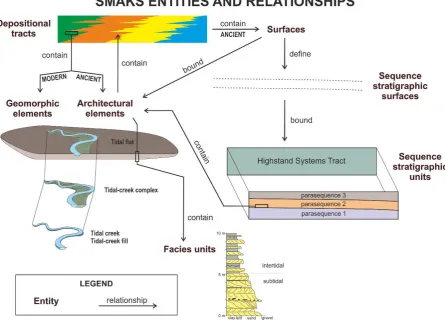
Figure 1: schematic representation of SMAKS entities and of the admissible relationships that may

exist between them. Relationships that are exclusively applicable to ancient or modern systems are

labelled as ‘ancient’ or ‘modern’, respectively.

Figure 2: Entity-relationship diagram that illustrates SMAKS entities (boxes) and relationships (lines);

5

line (in bold) denotes the entity name. For simplicity, look-up tables used for entity classifications are not represented in the figure.

SMAKS entities and relationships

This section illustrates the types of entities and relationships of SMAKS, explaining their geological meaning.

SMAKS case studies

A SMAKS case study is a dataset on a particular ancient or modern depositional system, as presented in a given published source (or set of related publications), or from original fieldwork. Therefore, the same depositional system may be the subject of different case studies. Different datasets can be merged in the same case study if the original authors intended their complementarity. It may be that the same dataset is presented across various publications. In such a case, each publication that contains part of the dataset are entered as a separate source, and all the sources that contain the dataset are stored as contributing to the same case study.

Case-study attributes (i.e., data fields organized as table columns) are stored in the table case_studies, whereas the table sources contains metadata on each published source, each of which can contain more than one case study (e.g., data on two different unrelated modern shelves).

SMAKS subsets

A subset is a part of a case study, defined flexibly on the basis of available constraints or types of observations with the particular scope of facilitating database interrogation. A subset may represent a particular stratigraphic volume (interval defined vertically and/or

horizontally, e.g., to account for proximal-distal variations, or for variations in some depositional-system parameters) of an ancient system, a plan-form segment of a modern system, or simply a portion of a dataset that should be differentiated in terms of the information it contains. Ultimately, subsets are erected to facilitate database query on parameters that describe the depositional systems and their boundary conditions, and on associated metadata.

The table subsets contain data on each subset, including both depositional-system parameters and metadata (see below).

SMAKS depositional tracts

A SMAKS ‘depositional tract’ for modern systems is defined as a plan-form belt that represents a gross depositional setting. For ancient systems it is defined as its preserved expression in the rock record, in the form of a sedimentary body that is continuous but potentially architecturally complex, and with boundaries that are time-transgressive and that may crosscut stratigraphic surfaces. The depositional tracts are units that are particularly – but not only – applicable to the largest-scale environmental subdivisions. The use of these units enables a lithostratigraphic approach: it allows the characterization of rock domains that represent the preserved product of a sub-environment but embody a potentially complex depositional history. The subdivision of strata into depositional tracts is determined by the observation of breaks in physical continuity displayed by deposits classifiable on

6

display physical continuity and are classifiable on depositional-tract types can be arbitrarily subdivided into depositional tracts. Arbitrary subdivision is carried out to allow for subset subdivision, or when a temporally intervening depositional tract has been distinguished. The temporal and spatial scales of these units are not defining characters for depositional-tract subdivision, but are attributes on which depositional tracts can be classified, thereby enabling comparison to be made for tracts that embody equivalent time-scales. The resolution of the depositional tracts is dictated in part by the subdivision of the stratigraphy into subsets, as all depositional tracts must be smaller or equivalent to the subsets in which they are contained. Multiple orders of depositional tracts can be erected for a case study, specifically to allow depositional tracts that crosscut different architectural elements to be defined, such as, for example, a front depositional tract that crosscuts several delta-lobe architectural elements (Fig. 3a). SMAKS depositional tracts largely correspond with the ‘facies tracts’ of several authors (e.g., Shanley & McCabe 1991; Gardner et al. 1992; Howell et al. 2008), and with the ‘zones’ of Vakarelov & Ainsworth (2013). Although depositional tracts are loosely defined in terms of genetic significance, they are particularly convenient for performing database filtering on environmental criteria, and represent useful containers of data that find application in reservoir-modelling practice (cf. MacDonald & Aasen 1994; Howell et al. 2008).

Every depositional tract can be classified according to environmental categories that are adopted in the original work (e.g., ‘coastal facies belt’), in an open-text field. Classification of the depositional tract is also possible in terms of environment of deposition according to alternative pre-defined classification schemes. Two predefined classification schemes are currently implemented in SMAKS. The categories contained within each scheme are mutually exclusive, but overlaps exist in the environmental types of the different schemes (e.g., ‘shoreface’ in classification scheme 1 potentially overlapping with ‘delta front’ in scheme 2). In application to the rock record, the classification of depositional tracts according to these schemes is based on interpretations provided in the original source works. Classification scheme 1 is based on the bathymetric zonation of the shoreline profile. If the term used to classify a unit in the original source work corresponds to any of the ones used in this classification scheme but with a different bathymetric significance, then either a re-classification is operated to maintain consistency in unit definition – whenever palaeo-bathymetric boundaries can be identified, and relying on the palaeo-palaeo-bathymetric

interpretations of the original authors – or the unit is left unclassified. The depositional tracts are left unclassified whenever reliable evidence of palaeo-bathymetry is missing. The categories included in this scheme, defined as in Reading & Collinson (1996), are:

‘backshore’, ‘foreshore’, ‘shoreface’, ‘offshore transition zone’, and ‘offshore’ (cf. Table 1). Classification scheme 2 is based on the physiographic zonation of deltas. The categories included in this scheme are: ‘delta top’, ‘delta front’, ‘prodelta’, and ‘incised-valley fill’ (cf. Table 1). The database structure allows addition of alternative and additional classification schemes at any time.

7

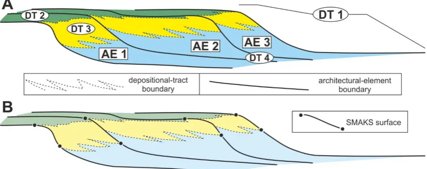
Figure 3: (A) Example of possible relationships between depositional tracts and architectural

elements, as seen along an idealized dip-oriented section: a ‘deltaic’ depositional tract (DT1: all the coloured domain) contains 3 ‘delta-lobe’ architectural elements (AE1-3) and lower-order ‘delta-top’,

‘delta-front’and ‘prodelta’ depositional tracts (DT2, DT3 and DT4, respectively) that themselves crosscut the architectural elements. (B) Ideal representation of how SMAKS surfaces may be contained in depositional tracts, and of how they may form the base or top (or a part thereof, in this particular example) of architectural elements. No vertical or horizontal scale implied.

SMAKS surfaces

For ancient successions, all surfaces that bound sedimentary bodies classifiable as architectural elements or sequence stratigraphic units (see below) at any scale can be stored in SMAKS. Each surface is contained in a depositional tract (which may be

unclassified), and may represent the base or top, or a part thereof, of architectural elements at multiple scales (Fig. 3b). Wherever a surface occurs at the top or base of a depositional tract, this relationship is recorded in a corresponding attribute. Wherever a surface crosscuts two laterally adjacent depositional tracts, this surface is broken down in two segments (Fig. 3b), and its effective continuity is stored in a table that describes relationships between surfaces (see below). Several surfaces can combine to define sequence stratigraphic surfaces of different type and hierarchical order.

All bounding surfaces, including sequence stratigraphic surfaces, can be classified according to classification schemes potentially adopted in the original source work, in terms of both nomenclature and hierarchy, in open-text fields. Two pre-defined classification schemes for the generic bounding surfaces are implemented in SMAKS (as of February 2016). One of the two schemes is based on objective characteristics (surfaces classified as: ‘sharp non -erosional’, ‘-erosional’, ‘structural’), whereas the other one is more interpretative (surfaces classified as: ‘wave ravinement’, ‘tidal ravinement’, ‘channel base’, ‘accretion surface’, ‘reactivation surface’, ‘growth fault’). A pre-defined classification scheme for sequence stratigraphic surfaces contains the following classes, as defined in Catuneanu et al. (2011) and references therein: ‘sequence boundary’, ‘maximum flooding surface’, ‘maximum

regressive surface, ‘wave ravinement surface’, ‘tidal ravinement surface’, ‘regressive surface of marine erosion’.

8

SMAKS sequence stratigraphic units

In SMAKS, sequence stratigraphic units include any hierarchical order of genetic units used to categorize the sequence stratigraphy of a succession. Sequence stratigraphic units at various orders can be contained within one another (e.g., parasequences within

parasequence sets; systems tracts within depositional sequences), defining a hierarchy of their own that can accommodate common sequence stratigraphic usage, and that is tailored to the particular dataset. Each largest-scale sequence stratigraphic unit is defined by its base and top; these are sequence stratigraphic surfaces. Therefore, sequence stratigraphic units are allowed to crosscut different depositional tracts and/or subsets (Fig. 4). In cases where architectural elements are attributed to a given sequence stratigraphic unit type, but there is no direct record of the surfaces that define the sequence stratigraphic unit, a

sequence stratigraphic unit with undefined surfaces but defined type can still be established. This facilitates database query (e.g., interrogation for all barrier-island elements in

transgressive systems tracts).

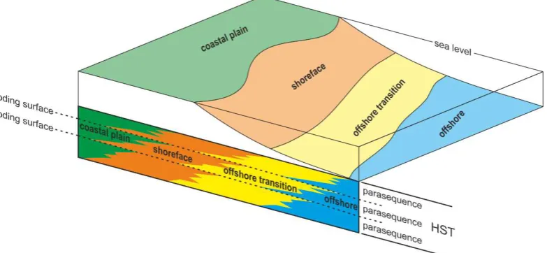
Figure 4: Ideal example of depositional tracts, as recognized in modern (planform) and ancient

(cross-section) depositional systems, and of the relationships between rock-record depositional tracts (coloured domains on cross section) and sequence stratigraphic surfaces (stippled lines) and units. The classes of depositional tracts reported in this ideal example are not representative of any predefined SMAKS classification, but only of how depositional-tract subdivision would be carried out based on categories adopted in the original source dataset. No vertical or horizontal scale implied.

Sequence stratigraphic units are classified on the hierarchical order of units they belong to, and on the type of unit at the particular level. Four pre-defined hierarchical levels are considered for the classification of sequence stratigraphic units: sequence, systems tract, parasequence set, and parasequence. Every sequence stratigraphic unit is classified according to categories that are adopted in the original work, which may include informal types that are not coded as a pre-defined class in SMAKS (e.g., ‘forced regressive systems tract’, ‘transgressive-regressive sequence’). Parasequence sets are classified as

9

1989). Given that sequence stratigraphic units are defined on the basis of the sequence stratigraphic surfaces that define their bases and tops, it is possible for any succession to be described in terms of both depositional sequences (bounded by sequence boundaries) and genetic stratigraphic sequences (bounded by maximum flooding surfaces) at the same time. All data on the sequence stratigraphic units are contained in the table

sequence_stratigraphic_units. SMAKS architectural elements

In SMAKS, architectural elements are discrete sedimentary bodies with characteristic facies associations and architectural properties (nature of bounding surfaces, external and internal geometries, stratal trends), interpretable as the preserved product of a sub-environment of deposition. As opposed to SMAKS depositional tracts, the use of these units enables an architectural approach (cf. Miall 1985), and allows the characterization of rock volumes that typically record the finite morphodynamic evolution of a geomorphological element (e.g., inception, growth and abandonment of a mouth bar; tidal sand ridge nucleation, migration and drowning). Exceptions include sedimentary bodies that record the unresolvable

amalgamation of identically classified elements. Each architectural element is contained in a depositional tract (which may be unclassified) and may be contained in a sequence

stratigraphic unit. For example, a mouth-bar architectural element may be contained in a delta-front depositional tract and may be attributed to a given parasequence. Architectural elements are permitted to contain lower-scale depositional tracts (e.g., delta-front

depositional tract contained within a delta-complex architectural element). The architectural elements themselves may belong to multiple scales, in a way that reflects the hierarchical arrangement of the sub-environments they represent (e.g., tidal channel-fill in tidal-flat deposits; delta lobes within a delta complex). This hierarchical organization is implemented in the form of a relative containment of architectural elements within other architectural elements. In some cases, the boundaries between different architectural elements may not be clear-cut, as a result of the gradual transition between preserved sub-environments. Here, the boundaries are defined as established in the original source work. This flexible approach to element subdivision facilitates the coding of a dataset, but entails uncertainty as to whether features of the coded elements are comparable. The hierarchical level of any architectural element in a case study can also be stored as an option by means of integer values, starting from ‘1’ for the lowest order (i.e., at smallest scale) of units in the dataset, in a pre-defined field. For example, an estuarine barform architectural element may be

assigned relative order ‘1’, whereas a higher-scale estuary fill in which it is contained may be assigned relative order ‘2’. This hierarchical classification is specific to each case, and allows for the inclusion of information on the hierarchical organization of sedimentary architecture that cannot be represented in terms of arrangement of lower-scale elements within higher-scale elements (e.g., data on hierarchy is given in the original work, but not explicitly provided in terms of relative containment of elements). Additionally, architectural elements can be classified according to the hierarchical levels proposed by Vakarelov & Ainsworth (2013), assigned following their criteria.

Architectural elements can be classified according to the categories of sub-environments that are adopted in the original work, in an open-text field. Assignment of architectural elements at multiple scales is based on the interpreted sub-environment of deposition

10

is possible at any time. Also, the categories in the scheme are not required to be mutually exclusive, as they are meant to be applicable to sub-environment types at various scales (e.g., chenier, chenier plain), and to the classification of geomorphic elements. The

attribution of any of these classes to a sedimentary body is based on the interpretation of the sub-environment of deposition, as given in the original source work, provided the definition of the sub-environment type matches with the definition chosen for SMAKS. Additionally, architectural elements can be classified according to element types proposed by Vakarelov & Ainsworth (2013), attributed following their criteria.

All data on the architectural elements are contained in the table architectural_elements. The sub-environment types are stored in the look-up table sub_environments.

SMAKS geomorphic elements

Geomorphic elements are discrete landforms that are characterized by distinctive

physiography, resulting from a particular set of depositional and erosional processes, and that represent different sub-environment types. Each geomorphic element is contained in a depositional tract (which may be unclassified). The elements may belong to multiple scales, in a way that reflects the hierarchical arrangement of the sub-environments they represent. Implementation of this hierarchical organization is in the form of a relative containment of geomorphic elements within other geomorphic elements. In some cases, sharp topographic breaks or clear-cut limits of any nature (e.g., change in surficial deposits) may be missing. The boundaries between different geomorphic elements are defined as established in the original source work. This flexible approach to element subdivision facilitates the coding of a dataset, but entails uncertainty as to whether the coded elements are comparable.

Geomorphic elements can be classified according to the categories of sub-environments that are adopted in the original work, in an open-text field. Geomorphic elements at multiple scales are also classified in terms of the interpreted sub-environment of deposition according to a classification scheme that contains a number of pre-defined categories. The

classification scheme is the same one adopted for the architectural elements (Table 1; Supplemental table 1), which is open-ended, allows addition of new categories, and contains element types that are applicable at multiple scales (e.g., ‘beach ridge’, ‘strandplain’). The classification of a geomorphological unit is based on the interpretation of the

sub-environment represented by the landform, as given in the original source work, provided the definition of the sub-environment type matches with the definition in the SMAKS scheme. Additionally, geomorphic elements can be classified according to element types proposed by Vakarelov & Ainsworth (2013), following their criteria.

11

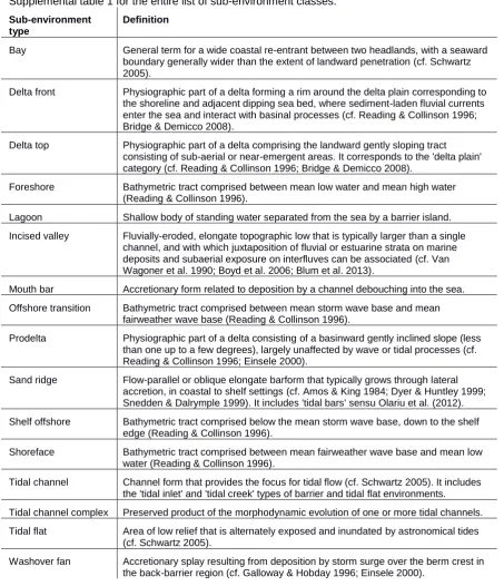
Table 1: Examples of SMAKS sub-environment types for the classification of architectural and geomorphic elements. Only the types discussed in this article are included here: see the Supplemental table 1 for the entire list of sub-environment classes.

Sub-environment type

Definition

Bay General term for a wide coastal re-entrant between two headlands, with a seaward boundary generally wider than the extent of landward penetration (cf. Schwartz 2005).

Delta front Physiographic part of a delta forming a rim around the delta plain corresponding to the shoreline and adjacent dipping sea bed, where sediment-laden fluvial currents enter the sea and interact with basinal processes (cf. Reading & Collinson 1996; Bridge & Demicco 2008).

Delta top Physiographic part of a delta comprising the landward gently sloping tract consisting of sub-aerial or near-emergent areas. It corresponds to the 'delta plain' category (cf. Reading & Collinson 1996; Bridge & Demicco 2008).

Foreshore Bathymetric tract comprised between mean low water and mean high water (Reading & Collinson 1996).

Lagoon Shallow body of standing water separated from the sea by a barrier island.

Incised valley Fluvially-eroded, elongate topographic low that is typically larger than a single channel, and with which juxtaposition of fluvial or estuarine strata on marine deposits and subaerial exposure on interfluves can be associated (cf. Van Wagoner et al. 1990; Boyd et al. 2006; Blum et al. 2013).

Mouth bar Accretionary form related to deposition by a channel debouching into the sea.

Offshore transition Bathymetric tract comprised between mean storm wave base and mean fairweather wave base (Reading & Collinson 1996).

Prodelta Physiographic part of a delta consisting of a basinward gently inclined slope (less than one up to a few degrees), largely unaffected by wave or tidal processes (cf. Reading & Collinson 1996; Einsele 2000).

Sand ridge Flow-parallel or oblique elongate barform that typically grows through lateral accretion, in coastal to shelf settings (cf. Amos & King 1984; Dyer & Huntley 1999; Snedden & Dalrymple 1999). It includes 'tidal bars' sensu Olariu et al. (2012).

Shelf offshore Bathymetric tract comprised below the mean storm wave base, down to the shelf edge (Reading & Collinson 1996).

Shoreface Bathymetric tract comprised between mean fairweather wave base and mean low water (Reading & Collinson 1996).

Tidal channel Channel form that provides the focus for tidal flow (cf. Schwartz 2005). It includes the 'tidal inlet' and 'tidal creek' types of barrier and tidal flat environments.

Tidal channel complex Preserved product of the morphodynamic evolution of one or more tidal channels.

Tidal flat Area of low relief that is alternately exposed and inundated by astronomical tides (cf. Schwartz 2005).

Washover fan Accretionary splay resulting from deposition by storm surge over the berm crest in the back-barrier region (cf. Galloway & Hobday 1996; Einsele 2000).

SMAKS facies units

12

relationships may not always be applicable: artificial transitions are recorded to account for the effective continuity of a facies unit across one or more elements (see below).

Again, facies units are classified according to the scheme adopted in the original source work, whereby lithofacies types are designated by codes; original lithofacies classes are stored in an open-text field. Common and generically applied classification schemes for the deposits are stored in closed fields. The grain size of the facies units is classified according to Folk’s (1954; 1980) textural classes (Fig. 5). Facies units are classified using Folk’s codes only when data or estimates on the proportion of each grain-size class to the total volume of the unit are given. Alternatively, whenever the lithotypes are classified only as ‘gravel’ (‘conglomerate’), ‘sand’ (‘sandstone’)or ‘mud’ (‘mudstone’), the grain size of the facies units should be classified as ‘-G’, ‘-S’ and ‘-M’, respectively. To permit distinction between

clay/claystone and silt/siltstone, the classes ‘C’ (clay) and ‘Z’ (silt) can be used instead of ‘M’ for sediment falling in the M field of Folk (1954; 1980). If heterolithic deposits are mapped as individual facies units, these can be classified as ‘G/S’, ‘S/G’, ‘S/M’, ‘M/S’ and ‘M/G’ (cf. Farrell et al. 2012). The modal grain size of sand-grade sediment is classified separately, as ‘very fine’ to ‘very coarse’. Organic deposits can be classified as ‘coal’ or ‘carbonaceous mudstone’.

Figure 5: Ternary diagram of Folk’s (1980) sediment texture categories. After Farrell et al. (2012).

A number of fields are employed to store data on sedimentary structures. The main internal structure of each facies unit is classified on two alternative schemes that each contain a number of pre-defined classes. The first scheme contains more specific categories (‘massive’, ‘asymmetrical ripple cross-lamination’, ‘symmetrical ripple cross-lamination’, ‘planar horizontal lamination’, ‘low-angle cross-bedding’, ‘trough cross-bedding’, ‘planar cross-bedding’, ‘flaser bedding’, ‘wavy bedding’, ‘lenticular bedding’, ‘swaley cross

13

or lamination, and grading. Attribute values describing secondary internal structures are contained in fields that relate deformation structures (‘slump folding’, ‘convolution’, ‘load structures’, ‘water-escape structures’, ‘synaeresis cracks’, ‘desiccation cracks’) and the facies-unit bioturbation index (Taylor & Goldring 1993).

All data relating to facies units are contained in the table facies_units. SMAKS subset statistics

In cases where data are derived from statistical summaries and cannot be referred to individual units, the statistics are stored as attributes of the entire subset. Descriptive statistics of geometrical parameters and of unit proportions, for groups of architectural and geomorphic elements of a given type, are stored in a separate table (subset_statistics). Hierarchical relationships between SMAKS entities

Hierarchical relationships between entities of a different rank (depositional tracts in subsets or architectural elements, architectural or geomorphic elements in depositional tracts,

architectural elements in sequence stratigraphic units, facies units in architectural elements), and between pairs of genetic units of the same rank (depositional tracts, architectural

elements, or geomorphic elements), but associated with different hierarchical levels, are expressed by means of numerical codes used to identify each individual unit (cf. Colombera et al. 2012a).

Spatial relationships between SMAKS genetic units

Spatial relationships between pairs of genetic units of the same rank (whether they be depositional tracts, architectural elements, facies units, and geomorphic elements) are stored in the form of transitions along the vertical, strike, and dip directions. The following conventions are adopted: vertical transitions are upward directed, dip transitions are downdip/offshore directed, strike transitions are right-hand lateral directed, facing offshore. Transitions are expressed by means of the numerical identifiers of the units (cf. Colombera et al. 2012a). Additional attributes used to describe each spatial relationship include the identifiers of the surface across which the transition is recorded, the nature of the transition (‘sharp’ or ‘gradual’, for elements and facies units), and the type of stratal termination (e.g., ‘updip onlap’, ‘downlap of upper unit’; for depositional tracts and architectural elements). For facies units, artificial transitions are recorded where the same facies unit effectively occurs at different positions within the element (e.g., sandstone bed traceable from ‘inner’ to ‘outer’ positions of an element), or where the same facies unit can be traced across more than one element.

These data are stored in four tables, one for each rank of units:

depositional_tract_transitions, architectural_element_transitions, facies_unit_transitions, and geomorphic_element_transitions.

Relationships between SMAKS surfaces

The relationships between two surfaces are expressed by means of the numerical identifiers of the surfaces. An attribute is used to specify a relationship of surface cross-cutting or whether two surfaces are effectively equivalent (artificial transition). This information is stored in the table surface_relationships. The correspondence of a generic surface with a portion of a sequence stratigraphic surface is recorded in the table

14

SMAKS attributes of genetic units and surfaces

This section provides some examples of the principal types of attributes associated with SMAKS sedimentary units and surfaces.

Geometrical parameters

Several types of morphometric parameters are adopted to describe the geometry of

depositional tracts, architectural elements, geomorphic elements and facies units. All these units are characterized in terms of their thickness, dip length (horizontal distance between the up-dip and down-dip boundaries of a unit, as measured within the unit) and strike width (horizontal distance between the boundaries of a unit as measured along depositional strike). These parameters are classified by observation type (e.g., as ‘real’, ‘apparent’; ‘partial’, ‘unlimited’, sensu Geehan & Underwood, 1993). All the dimensional parameters are explained further in the supplemental material. Additional geometrical attributes are

applicable to particular unit types. These include, for example, the ‘shoreline trajectory’ associated to a depositional tract, i.e. the angle that defines the direction of migration of a depositional shoreline-break, sensu Posamentier & Vail 1988, as measured relative to the palaeo-horizontal (cf. Helland-Hansen & Martinsen 1996; Hampson et al. 2009; see

Supplemental text), and descriptors of the three-dimensional shape of architectural elements and facies units, or of the morphology of geomorphic elements (see Supplemental text). A fuller description of SMAKS genetic-unit geometrical parameters is provided in the

Supplemental text. Other attributes

A number of other attributes are used to characterize SMAKS units and store associated metadata. The system is extendable; additional attributes can be added at any time. By way of example, some of SMAKS genetic-unit attributes include: a ‘process category’ that

classifies the interpreted relative importance played by wave, tidal and fluvial processes in depositing and shaping architectural and geomorphic elements, as defined in Ainsworth et al. (2011; e.g., ‘Twf’ = tide dominated, wave influenced, fluvial affected); a ‘data quality index’ used to implement a threefold ranking system (cf. Baas et al. 2005; Colombera et al. 2012a) of the degree to which existing data support the sub-environment interpretation of the architectural elements; a classification of the unidirectional or bidirectional (oscillatory or combined flow) character of the (palaeo-) flow recorded in a sedimentary body or associated with geomorphological units; two alternative ‘accretion types’, which classify the style of accretion of architectural or geomorphic elements, relative to the dominant (palaeo-) flow direction or to the shoreline, respectively; the ‘timescale’ (e.g., 104 _yr) and ‘duration’ _(e.g., 16500 yr) of a unit, as inferred from existing temporal constraints; five alternative

classifications of the position of a facies unit within its parent architectural element, in terms of bathymetric/physiographic setting (cf. Supplemental figure 5), tidal zone, or relative distality; multiple ‘trace fossil’ fields, used to specify the presence of a particular ichnogenus in a facies unit, both ‘mean aggradation rate’ and ‘mean progradation rate’, of some

15

SMAKS attributes of case studies and depositional systems

A varied suite of data fields is deployed to store metadata associated with SMAKS published sources, case studies, depositional systems and subsets. Metadata include information such as the type of data source (e.g., peer-reviewed scientific articles, unpublished academic works), the geographical location of a case study, the methods of data acquisition (e.g., outcrop observations, high-resolution seismic surveys), the chronostratigraphic attribution of stratigraphic intervals, the suitability of a given subset for the retrieval of a particular type of output, the perceived data quality ('data quality index'; cf. Baas et al. 2005; Colombera et al. 2012a).

Other attributes are used to store data on (i) parameters that describe intrinsic

characteristics of the depositional systems and their subsets (e.g., shelf width, depositional gradient, mean aggradation rate, duration), and (ii) the variables that are thought to act as controlling factors to these systems (e.g., tectonic setting, palaeolatitude at time of

deposition, mean significant wave height, coastal tidal range). Depositional-system

controlling factors are assigned based on proxies and constraints that are independent from interpretations of sedimentary architecture.

Database interrogation and example output

As of February 2016, SMAKS contains data on 27 case studies, derived from 47 published sources (see Table 2). The database can be interrogated by means of Structured Query Language (SQL) queries to generate quantitative information on the sedimentary

architecture and geomorphological organization of shallow-marine to paralic depositional systems. All the data can be filtered on the parameters used to classify the depositional systems (e.g., selection of rift basins, macrotidal coasts, seas with wave power density lower than 10 kW/m), as well as on all the associated metadata (e.g., selection of datasets based on outcrop studies, Cretaceous systems, data collected after 1990), to facilitate the selection of appropriate analogues. This information can then be exported to spreadsheets in a format suitable for analysis and presentation.

The database output allows a characterization of the organization of depositional systems and of their formative sedimentary and geomorphological units at multiple scales, in terms of hierarchical relationships, proportions, geometry, spatial relationships and distributions of lower-order genetic units in higher-order packages.

Eight example sets of SMAKS output are presented below with the purpose of

16

Table 2: summary of SMAKS case studies, with abbreviated references to published data sources. The case studies are ordered by identifier (column ‘ID’), which is assigned sequentially, and therefore

reflects the chronological order of addition to the database. The informal name given to the case

studies (column ‘Case study’) may appear twice because different datasets by different authors but on

the same succession or sea may be present in SMAKS.

ID Case study Location Source reference

1 Star Point Sandstone Utah, USA Hampson et al. (2011)

2 Po Delta Italy Correggiari et al. (2005a)

Correggiari et al. (2005b)

3 Mississippi Delta Louisiana, USA Frazier (1967)

Roberts (1997)

4 Composite database - Reynolds (1999)

5 Ebro Delta Spain Somoza et al. (1998)

6 Ferron Sandstone 'Notom Delta' Utah, USA Li et al. (2010)

Li et al. (2011a)

Li et al. (2011b)

Li et al. (2012)

Zhu et al. (2012)

7 Composite database - Off (1963)

8 East China Sea East China Sea Liu et al. (2000)

Berné et al. (2002)

Liu et al. (2007)

9 East China Sea East China Sea Yang (1989)

10 Upper Cibulakan Formation Java Sea Posamentier (2002)

11 East Bank, North Sea North Sea Davis & Balson (1992)

12 Bering Sea Bering Sea Nelson et al. (1980)

13 Eastern Yellow Sea Yellow Sea Park & Lee (1994)

14 Korea Strait Korea Strait Park & Lee (1994)

15 Korea Strait Korea Strait Park et al. (2003)

16 Eastern Yellow Sea Yellow Sea Park et al. (2006)

17 Eastern Yellow Sea Yellow Sea Klein et al. (1982)

18 Southern North Sea North Sea Trentesaux et al. (1994)

Berné et al. (1994)

Trentesaux et al. (1999)

19 Southern North Sea North Sea Houbolt (1968)

Caston (1972)

20 Gulf of Khambhat Arabian Sea Saha et al. (2007)

21 Western Yellow Sea Yellow Sea Liu et al. (1989)

22 East China Sea East China Sea Yoo et al. (2002)

23 Southern North Sea North Sea Tessier et al. (1999)

24 Celtic Sea Celtic Sea Bouysse et al. (1976)

17

Pantin & Evans (1984)

Scourse et al. (2009)

25 Celtic Sea Celtic Sea Berné et al. (1998)

Marsset et al. (1999)

Reynaud et al. (1999)

Reynaud et al. (2003)

26 Yellow River Delta China Xue (1993)

van Gelder et al. (1994)

Li et al. (1998)

Wang et al. (2015)

27 Ferron Sandstone 'Last Chance Delta' Utah, USA Garrison & van den Bergh (2004)

van den Bergh & Garrison (2004)

Example 1: determining net-to-gross ratios for prediction of uncertainty in reservoir quality The database can be applied to determine the ranges of net-to-gross ratios that are typically seen in types of architectural elements that form the building blocks of deltaic strata, as represented in Fig. 6a. Such an interrogation could be based on facies-unit proportions and on user-defined specifications of net and non-net facies-unit categories. Such data, compiled from multiple analogues, and referring to features at different scales, could be applied to make predictions of uncertainty in reservoir net-to-gross ratio for different physiographic features identifiable on seismic lines (e.g., delta front, prodelta) or for objects that may be below seismic resolution (e.g., mouth bars). Because the database records the spatial relationships between genetic units, corresponding data could be retrieved for sets of

spatially and genetically related units in terms of relative net-to-gross ratios of delta-front and prodelta deposits, for example (Fig. 6b). Such information could be applied to attempt

predictions of net-to-gross ratios away from well control in updip and downdip directions, where prodelta and delta-front deposits are sampled, respectively.

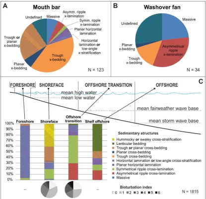
Example 2: information on facies organization of distinct sub-environments

The total proportions of the different facies-unit types seen within depositional tracts or architectural elements provide base-case facies models. These can be used to describe the likelihood of occurrence of different types of grain-size categories and associated

18

Figure 6: (A) Box plots that describe the distribution of the net-to-gross ratios of 58 architectural elements classified as ‘prodelta’, ‘delta front’ or ‘mouth bar’ elements. These net-to-gross ratios are computed by SMAKS based on proportions that relate the total measured thickness of different types of grain-size classes of facies units, and on user-specified non-net facies unit types (muddy

lithofacies). Boxes represent interquartile ranges, horizontal bars within them represent median values, crosses (x) represent mean values, and spots represent outliers. (B) scatter-plot that relates the net-to-gross ratio of delta-front deposits with the net-to-gross ratio of downdip transitional prodelta deposits. The datapoints are colour-coded by depositional system (Quaternary Po delta, Italy; Last Chance Delta and Notom Delta intervals of the Ferron Sandstone, Upper Cretaceous, USA). See Table 2 for data sources.

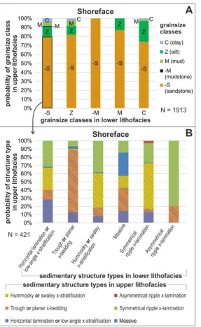
Example 3: transition statistics that describe the spatial relationships in three dimensions of unit types within higher-order packages

The facies-unit information of example 2, above, can be coupled with output that describes the likely vertical stacking and degree of mutual association of lithofacies types within successions interpretable in terms of the same sub-environment types (Fig. 9). Again, transition statistics could be obtained for SMAKS grain-size categories (Fig. 9a), or for the types of internal sedimentary structures seen in sand-prone facies units (Fig. 9b), for example. Fig. 9 only represents first-order transition statistics (i.e., evaluated across

19

Example 4: detailed information on the grain-size of facies units in depositional tracts and architectural elements

The granulometric characterization of lithofacies can be refined by querying for data on the modal size of sandy facies units, and for statistical parameters that describe the grain-size distribution (cf. Folk 1966; and references therein). As an example, the output in Fig. 10 shows grain-size data for facies units from Quaternary architectural elements classified as shelf tidal sand ridges, from six different locations. Together with data of the types shown in examples 2 and 3, this type of output contributes to the compilation of quantitative facies models, which may find application as templates for assisting with sub-environment

interpretation of ancient deposits. The discrimination of grain-size domains based on textural parameters can also be applied to the determination of autogenic behaviours of

granulometric segregation in different element types, or to the assessment of the sensitivity of grain-size parameters, and resulting petrophysical heterogeneity, to specific controlling factors.

Example 5: information on the internal organization of sequence stratigraphic units

Fig. 11 illustrates output that characterizes the geometry of nearshore sandstone belts within Upper Cretaceous parasequences of the Western Interior Seaway (Utah, USA). The

20

21

Figure 8: Proportions of dominant internal sedimentary structures in sandy facies units from different

22

Figure 9: (A) Bar chart that quantifies the frequency with which the grain-size class of a facies-unit

(colour-coded and labelled in the bars) is vertically stacked on facies units with grain-size class labelled on the horizontal axis, as seen within architectural elements classified as ‘shoreface’ (see

23

Figure 10: (A) Thickness-based proportions of sand granulometric classes in sandy facies units for

groups of shelf tidal sand ridges from six different locations. (B) Grain-size mean and standard deviation for sandy facies units from shelf tidal sand ridges, colour-coded by location. See Table 2 for data sources.

Example 6: information on the geometry of architectural elements at multiple hierarchical levels, corresponding to different scales of observation

The example output in Fig. 12 illustrates the geometry of architectural elements that form the constructional units of four Quaternary deltas at multiple scales, and highlights some

relationships existing between spatial scale, temporal scale, and hierarchical arrangement of the units in terms of relative containment of architectural elements. Furthermore, the

example in Fig. 12 shows the ability to query the database for units that are solely classified following nomenclatures adopted in the original source works (i.e., at the time of data entry, no equivalent term or element type existed in the SMAKS classification of sub-environments, which is expandable). The analysed literature studies, on which Figure 12 is based,

recognized a hierarchy of constructional deltaic units; each of these studies erected a nomenclature of its own for units belonging to the different orders. This analysis highlights the use of a common term: the ‘delta lobe’. A delta lobe is not defined on universally

24

defined in genetic terms. Thus, this example output provides an indication of the value of the database as a tool with which to undertake comprehensive analyses of the hierarchical organization in the sedimentary architecture of clastic depositional systems and of the associated terminology.

Figure 11: (A) scatter-plot of dip length versus thickness for parasequence-scale nearshore

sandstones, based on data derived from outcrop studies; a power-law regression curve is fit to the data. (B) scatterplot of dip length versus progradation angle for parasequence nearshore sandstones; the field of negative progradation angle (forced regression) is expanded in C, in which an exponential regression curve is fit to the data; the field of positive progradation angle (depositional regression) is expanded in D, in which a power-law regression curve is fit to the data. All data are from exhumed successions in the Upper Cretaceous of the Western Interior Seaway (Utah, USA); see Table 2 for data sources.

Example 7: information on the morphometry of geomorphic elements

Output on the geometry of SMAKS genetic units can be queried in the form of descriptive statistics, enabling comparisons with datasets that were originally provided in the form of statistical parameters, which are also stored in SMAKS as subset statistics. As an example, descriptive statistics of the morphometry of modern tidal sand ridges based on an analysis of bathymetric datasets carried out in the early 1960s (Off 1963) are compared with

25

morphodynamic evolution on the geometry of sedimentary bodies that may form reservoir units or stratigraphic traps.

Figure 6: (A) Scatter-plot of architectural-element width and thickness for deltaic constructional units

at multiple scales, and originally categorized following different nomenclatures, from four different Quaternary deltas; all data are based on subsurface interpretations. (B) Scatter-plot of architectural-element dip length and width for deltaic constructional units. (C) Scatter-plot of the thickness of

architectural elements originally classified as ‘delta lobe’ (horizontal axis) versus the thickness of the higher-scale architectural elements in which they are contained (vertical axis); the spots are coloured according to the classification of the higher-scale elements, as in legend. (D) Scatter-plot of

architectural-element thickness versus the duration of deposition, as inferred from existing temporal constraints, for deltaic units at multiple scales.

Example 8: integration of sedimentological and geomorphological information

26

relationship with present-day coastal processes. However, this information serves as an example of how output of this type will allow for testing and developing models that account for the sensitivity of sedimentological products to their controlling factors.

These 8 summary examples are intended to showcase some of the possible database capabilities and applications, and are by no means exhaustive.

Figure 13: (A) representation of morphometric parameters of a tidal sand ridge, intended as

27

Discussion: database applications

The SMAKS database can yield output with which to undertake an empirical characterization of many analogues, from which quantitative models, or rules that describe the heterogeneity of reservoir types, can be derived. This application can enable the identification of

correlations between different architectural properties (e.g., predicted vs. measured; cf. Fig. 11a) and predictions of reservoir characteristics away from data coverage (e.g., variations in net-to-gross ratio within and across sedimentary units; cf. Fig. 6).

The ability to query for sedimentological properties and to apply filters to the database output permits the selection of analogues that share user-specified characteristics, which could be sedimentological characteristics (e.g., occurrence of a particular facies association) or parameters that describe the depositional context (e.g., basin type, coastal tidal range), or both. The synthesis of quantitative information from multiple case studies results in the construction of composite analogues, which incorporate variability in sedimentological and stratigraphic properties (cf. Fig. 6a), and are therefore suitable for the quantification of associated uncertainty. These composite analogues are adoptable as quantitative facies models (cf. Baas et al. 2005; Colombera et al. 2013) that have been proven to be useful for the definition of conceptual models of reservoir heterogeneity, for conditioning stochastic geocellular reservoir models (cf. Colombera et al. 2012b), and for guiding well-to-well correlations of sandbodies or mudstone units (Colombera et al. 2014; 2016).

Furthermore, the devised database addresses the necessity for the integration of datasets that are heterogeneous and in part interdisciplinary (cf. Parsons et al. 2011), and this will likely facilitate the application of meta-analysis (Borenstein et al. 2009) as a research

approach in sedimentary geology. In the recent past, it has been shown that the compilation of composite datasets arising from multiple case studies and their use in comparative analyses may yield novel insight into the sensitivity of sedimentological products to different forcing mechanisms (e.g., Macklin et al. 2012; Colombera et al. 2015; Hamylton & Puotinen 2015).

Some of the example output presented above indicates the potential of this database for fundamental research based on meta-analysis (cf. Fig. 11, 13c). There exists a need for standardization in classifications and attribute definitions, particularly in terminology-rich disciplines like the Earth Sciences, if such meta-studies are to be conducted with rigour (cf. Barchyn et al. 2011). In the methodology used for SMAKS, this need is addressed by enforcing the translation of different datasets to a common standard. However, a translation of entity attributes (e.g., class of sub-environment) to a common standard is not achievable in some cases because complex terminologies exist and these are commonly applied inconsistently (e.g., terms recurring in different nomenclatures but with different definitions). A database system of this type should facilitate the review and analysis of the varied

terminology adopted in the published literature (cf. Fig. 12c), and may therefore find application in highlighting discrepancies and pitfalls in current sedimentological practice.

Conclusions

28

been structured with consideration of the variety of approaches and data types that are taken in studying the sedimentary geology of shallow-marine and paralic depositional

systems. The database allows for a convergence of datasets from studies of outcrops, of the subsurface and of the modern seabed. This convergence permits the reconciliation of facies analysis, architectural-element analysis, sequence stratigraphy and geomorphology.

Example database output has been shown to demonstrate the type of information that can be obtained upon interrogation, the depositional spectrum covered by the database, the wide variety of data types considered, the ability to reconcile different approaches under a common framework, and the ability to deal with different nomenclatures and classifications. The example output has also been selected to show the value of the database as (i) a resource that may find application in subsurface studies, in contexts of hydrocarbon exploration, development and production, and (ii) a research tool that can facilitate a meta-analysis approach whereby process-response models of shallow-marine depositional systems can be tested through the simultaneous analysis of multiple case studies.

Acknowledgements

NERC is thanked for financial support of this research (Catalyst Fund award

NE/M007324/1). The Shallow-Marine Research Group is also supported by Debmarine and Engie. Tony Reynolds and Gary Hampson are thanked for their helpful reviews, which improved the paper.

References

Ainsworth, R. B., Vakarelov, B. K., & Nanson, R. A. (2011). Dynamic spatial and temporal prediction of changes in depositional processes on clastic shorelines: Toward improved subsurface uncertainty reduction and management. AAPG Bulletin, 95, 267-297.

Amos, C. L., & King, E. L. (1984). Bedforms of the Canadian eastern seaboard: a comparison with global occurrences. Marine Geology, 57, 167-208.

Baas, J. H., McCaffrey, W. D., & Knipe, R. J. (2005). The Deep-Water Architecture

Knowledge Base: towards an objective comparison of deep-marine sedimentary systems. Petroleum Geoscience, 11, 309-320.

Barchyn, T. E., Hugenholtz, C. H., & Ellis, J. T. (2011). A call for standardization of aeolian process measurements: moving beyond relative case studies. Earth Surface Processes and Landforms, 36, 702-705.

Berné, S., Trentesaux, A., Stolk, A., Missiaen, T., & De Batist, M. (1994). Architecture and long term evolution of a tidal sandbank: The Middelkerke Bank (southern North Sea). Marine Geology, 121, 57-72.

Berné, S., Lericolais, G., Marsset, T., Bourillet, J. F., & De Batist, M. (1998). Erosional offshore sand ridges and lowstand shorefaces: examples from tide-and wave-dominated environments of France. Journal of Sedimentary Research, 68, 540-555.

29

Blum, M., Martin, J., Milliken, K., & Garvin, M. (2013). Paleovalley systems: Insights from Quaternary analogs and experiments. Earth-Science Reviews, 116, 128-169.

Borenstein, M., Hedges, L. V., Higgins, J., & Rothstein, H. R. (2009). Introduction to meta-analysis. Wiley, Chichester. 421 pp.

Bouysse, P., Horn, R., Lapierre, F., & Le Lann, F. (1976). Etude des grands bancs de sable du Sud-Est de la Mer Celtique. Marine Geology, 20, 251-275.

Boyd, R., Dalrymple, R. W., & Zaitlin, B. A. (2006). Estuary and incised valley facies models. In: Posamentier, H. W., & Walker, R. G. (Eds.) Facies Models Revisited. SEPM Special Publication, 84, 171-234.

Bridge, J., & Demicco, R. (2008). Earth surface processes, landforms and sediment deposits. Cambridge University Press. 815 pp.

Carle, S. F., & Fogg, G. E. (1997). Modeling spatial variability with one and multidimensional continuous-lag Markov chains. Mathematical Geology, 29, 891-918.

Caston, V. N. D. (1972). Linear Sand Banks in the Southern North Sea. Sedimentology, 18, 63-78.

Catuneanu, O., Galloway, W. E., Kendall, C. G. St. C., Miall, A. D., Posamentier, H. W., Strasser, A., & Tucker, M. E. (2011). Sequence stratigraphy: methodology and

nomenclature. Newsletters on Stratigraphy, 44, 173-245.

Chen, P. P. S. (1976). The entity-relationship model—toward a unified view of data. ACM Transactions on Database Systems (TODS), 1, 9-36.

Colombera, L., Mountney, N. P., & McCaffrey, W. D. (2012a). A relational database for the digitization of fluvial architecture concepts and example applications. Petroleum Geoscience, 18, 129-140.

Colombera, L., Felletti, F., Mountney, N. P., & McCaffrey, W. D. (2012b). A database approach for constraining stochastic simulations of the sedimentary heterogeneity of fluvial reservoirs. AAPG Bulletin, 96, 2143-2166.

Colombera, L., Mountney, N. P., & McCaffrey, W. D. (2013). A quantitative approach to fluvial facies models: Methods and example results. Sedimentology, 60, 1526-1558. Colombera, L., Mountney, N. P., Felletti, F., & McCaffrey, W. D. (2014). Models for guiding and ranking well-to-well correlations of channel bodies in fluvial reservoirs. AAPG Bulletin, 98, 1943-1965.

Colombera, L., Mountney, N. P., & McCaffrey, W. D. (2015). A meta-study of relationships between fluvial channel-body stacking pattern and aggradation rate: Implications for sequence stratigraphy. Geology, 43, 283-286.

Colombera, L., Mountney, N. P., Howell, J. A., Rittersbacher, A., Felletti, F., & McCaffrey, W. D. (2016). A test of analog-based tools for quantitative prediction of large-scale fluvial

architecture. AAPG Bulletin, 100, 237-267.

30

Correggiari, A., Cattaneo, A., & Trincardi, F. (2005b). The modern Po Delta system: lobe switching and asymmetric prodelta growth. Marine Geology, 222, 49-74.

Cowell, P. J., Roy, P. S., Cleveringa, J., & de Boer, P. l. (1999). Simulating coastal systems tracts using the shoreface translation model. In: Harbaugh, J. W., Watney, W. L., Rankey, E. C., Slingerland, R., Goldstein, R. H., & Franseen, E. K. (eds.), Numerical experiments in stratigraphy: Recent advances in stratigraphic and sedimentologic computer simulations. SEPM Special Publication, 42, 371-380.

Davis Jr, R. A., & Balson, P. S. (1992). Stratigraphy of a North Sea tidal sand ridge. Journal of Sedimentary Research, 62, 116-121.

Dowey, P. J., Hodgson, D. M., & Worden, R. H. (2012). Pre-requisites, processes, and prediction of chlorite grain coatings in petroleum reservoirs: A review of subsurface examples. Marine and Petroleum Geology, 32, 63-75.

Dreyer, T., Fält, L. M., Høy, T., Knarud, R., & Cuevas, J. L. (1993). Sedimentary architecture of field analogues for reservoir information (SAFARI): a case study of the fluvial Escanilla Formation, Spanish Pyrenees. In: Flint, S. S., & Bryant, I. D. (eds.) The geological modelling of hydrocarbon reservoirs and outcrop analogues. IAS Special Publication, 15, 57-80.

Dyer, K. R., & Huntley, D. A. (1999). The origin, classification and modelling of sand banks and ridges. Continental Shelf Research, 19, 1285-1330.

Einsele, G. (2000). Sedimentary basins: Evolution, facies, and sediment budget. Springer-Verlag, Berlin. 792 pp.

Evans, C. D. R., & Hughes, M. J. (1984). The Neogene succession of the South Western Approaches, Great Britain. Journal of the Geological Society, 141, 315-326.

Farrell, K. M., Harris, W. B., Mallinson, D. J., Culver, S. J., Riggs, S. R., Pierson, J., Self-Trail, J. M., & Lautier, J. C. (2012). Standardizing texture and facies codes for a process-based classification of clastic sediment and rock. Journal of Sedimentary Research, 82, 364-378.

Folk, R. L. (1954). The distinction between grain size and mineral composition in sedimentary-rock nomenclature. The Journal of Geology, 344-359.

Folk, R. L. (1966). A review of grain size parameters. Sedimentology, 6, 73-93. Folk, R. L., 1980. Petrology of sedimentary rocks. Hemphill, Austin. 182 pp.

Frazier, D. E. (1967). Recent deltaic deposits of the Mississippi River: their development and chronology. Transactions of the Gulf Coast Association of Geological Societies, 17, 287-315. Galloway, W. E. (1989). Genetic stratigraphic sequences in basin analysis I: architecture and genesis of flooding-surface bounded depositional units. AAPG Bulletin, 73, 125-142.

Galloway, W. E., & Hobday, D. K. (1996). Terrigenous clastic depositional systems: Applications to fossil fuel and groundwater resources. Springer, New York. 489 pp. Gardner, M. H., Barton, M. D., Tyler, N., & Fisher, R. S. (1992). Architecture and

31

Garrison Jr, J. R., & van den Bergh, T. C. V. (2004). High-resolution depositional sequence stratigraphy of the upper Ferron Sandstone Last Chance Delta: an application of coal-zone stratigraphy. In: Chidsey Jr, T. C., Adams, R. D., & Morris, T. H. (eds.) Regional to wellbore analog for fluvial-deltaic reservoir modeling: The Ferron Sandstone of Utah: AAPG Studies in Geology, 50, 125-192.

Geehan, G., & Underwood, J. (1993). The use of length distributions in geological modelling. In: Flint, S. S., & Bryant, I. D. (eds.) The geological modelling of hydrocarbon reservoirs and outcrop analogues, IAS Special Publication, 15, 205-212.

Gibling, M. R. (2006). Width and thickness of fluvial channel bodies and valley fills in the geological record: a literature compilation and classification. Journal of sedimentary Research, 76, 731-770.

Hampson, G. J., Sixsmith, P. J., Kieft, R. L., Jackson, C. A. L., & Johnson, H. D. (2009). Quantitative analysis of net transgressive shoreline trajectories and stratigraphic

architectures: mid to late Jurassic of the North Sea rift basin. Basin Research, 21, 528-558. Hampson, G. J., Gani, M. R., Sharman, K. E., Irfan, N., & Bracken, B. (2011). Along-strike and down-dip variations in shallow-marine sequence stratigraphic architecture: Upper Cretaceous Star Point Sandstone, Wasatch Plateau, Central Utah, USA. Journal of Sedimentary Research, 81, 159-184.

Hamylton, S. M., & Puotinen, M. (2015). A meta analysis of reef island response to

environmental change on the Great Barrier Reef. Earth Surface Processes and Landforms, 40, 1006-1016.

Harris, P. T., & Whiteway, T. (2011). Global distribution of large submarine canyons: Geomorphic differences between active and passive continental margins. Marine Geology, 285, 69-86.

Helland-Hansen, W., & Martinsen, O. J. (1996). Shoreline trajectories and sequences; description of variable depositional-dip scenarios. Journal of Sedimentary Research, 66, 670-688.

Helle, K., & Helland Hansen, W. (2009). Genesis of an over thickened shoreface sandstone tongue: The Rannoch and Etive formations of the Middle Jurassic Brent delta, North Sea. Basin Research, 21, 620-643.

Houbolt, J. J. H. C. (1968). Recent sediments in the southern bight of the North Sea. Geologie en Mijnbouw, 47, 245-273.

Howell, J. A., Skorstad, A., MacDonald, A., Fordham, A., Flint, S., Fjellvoll, B., & Manzocchi, T. (2008). Sedimentological parameterization of shallow-marine reservoirs. Petroleum Geoscience, 14, 17-34.

Howell, J. A., Martinius, A. W., & Good, T. R. (2014). The application of outcrop analogues in geological modelling: a review, present status and future outlook. In: Martinius, A. W.,

Howell, J. A., & Good, T. R. (eds.) Sediment-body geometry and heterogeneity: analogue studies for modelling the subsurface. Geological Society, London, Special Publications, 387, 1-25.

Jung, A., & Aigner, T. (2012). Carbonate geobodies: Hierarchical classification and