Extraction and interaction analysis of foreground objects in panning video

(1)

Rochester Institute of Technology

RIT Scholar Works

Theses Thesis/Dissertation Collections

2006

Extraction and interaction analysis of foreground

objects in panning video

Raja Jain

Follow this and additional works at:http://scholarworks.rit.edu/theses

This Thesis is brought to you for free and open access by the Thesis/Dissertation Collections at RIT Scholar Works. It has been accepted for inclusion in Theses by an authorized administrator of RIT Scholar Works. For more information, please [email protected].

Recommended Citation

(2)

Extraction and Interaction Analysis of Foreground

Objects in Panning Video

by

Raja P. Jain

Thesis report submitted in partial fulfillment of the requirements of the degree of Master of Science in Computer Science

Department of Computer Science

B.Thomas Golisano College of Computing and Information Sciences Rochester Institute of Technology

Rochester, New York May 2006

Approved By:

________________________________________________________________________ Dr. Roger S. Gaborski

Professor, Department of Computer Science Advisor

________________________________________________________________________ Dr. Carl H. Reynolds

Professor, Department of Computer Science Reader

________________________________________________________________________ Dr. Peter G. Anderson

(3)

Acknowledgements

I am thankful to my parents and brother for supporting me through my master’s

(4)

Abstract

In this work, moving foreground objects are extracted from video. The video camera can be either stationary or panning. The motion information extracted from consecutive frames of video is used for object segmentation, and an appearance model of the moving object is created. No assumptions are made concerning the object model, resulting in segmented objects of varying shapes and sizes. Finally, relationships between objects in the image are evaluated toward the goal of higher level understanding of videos.

Objectives

1) Extracting moving foreground objects in a video taken from either stationary or moving camera.

2) Finding the relative velocity of the moving foreground objects in the video. 3) Segmenting the moving foreground objects using motion, distance, and object

relationships obtained from few consecutive frames of video. The color information doesn’t play a major role in object segmentation, resulting in a system which is able to segment foreground objects having very similar color and texture as that of the background.

4) Generating appearance model of the moving objects, i.e., determining the ranges of colors present in moving objects. The algorithm is able to determine what colors are present in the segmented moving foreground objects. The system can search and highlight the objects having specified color and can also highlight the particular part of the objects having the specified color.

5) Extracting the spatial relationship between any two segmented moving objects. This is a step towards higher level understanding of the videos. Based on this work, a system can be made which can search the videos based on the queries specifying the spatial relationships among the objects such as, “find the videos where 2 objects meet each other”, “find the videos in which one object is

following the other object”, “find the videos where 2 objects meet each other and the go away/together”, etc.

(5)

Segmenting moving objects in video is a fundamental step in the process of developing an automated computer vision system for higher level understanding of the videos. For achieving higher level understanding of videos, the system should be able to extract interesting objects from the sequence of frames and should be able to develop a content-based description of video, establish relationships between the interesting objects and generate meaningful information from them. It can have a variety of applications such as video surveillance, gesture recognition, traffic monitoring, etc. Examples of video

surveillance are detecting suspicious behavior in parking lots, interaction between people in public places such as restaurants, and speeding and suspiciously moving cars, etc. Once object segmentation is accomplished, a system for object recognition can be made on the top of it and the system can be used in applications such as regularizing

pedestrians and highway traffic using density evaluations obtained from segmenting moving people and vehicles.

Also, the recent techniques in image/video coding, segment image/videos into objects to and achieve high compression by separately coding the contour and texture of those objects. Since the sole purpose is to achieve efficient compression, the segmented objects may not be semantically meaningful to humans. Other applications such as content based video retrieval require the segmented objects to be semantically meaningful to the human observers.

An ideal object segmentation system should be able to identify the semantically

meaningful components of the image and should be able to group the pixels belonging to such components. It is difficult to segment the static objects in the video, but moving objects can be segmented by using their motion information along with other

information.

1.2 Definition of the Problem

This work addresses the problem of extracting moving objects from the video taken with either stationary or panning camera, generating their appearance model, and trying to establish spatial relationships among them. No assumptions are made concerning the object model, so the system should be able to detect moving objects of varying shapes and sizes. Moving objects are segmented primarily from the motion-based information and the relationship they maintain over a certain number of frames. Since the

(9)

segment it since color information doesn’t play a major role in object segmentation. Also the system is able to tell what ranges of color are present in the car, i.e., it generates the appearance model of the car.

The information such as location of objects in each frame, ranges of color present in the object, relative velocity of the objects, and the number of frame when the objects entered and left the scene can be used to generate spatial relationships between the objects. Generating the spatial relationship among the moving foreground objects is a step towards higher level understanding of the videos.

The source code was developed using Intel’s OpenCV library [30] in Microsoft’s VC++ 6.0 IDE on Windows XP platform.

1.3 Thesis Outline

In chapter 1, definition of the problem and application of the problem in various fields of computer vision is explained.

The first step in solving the problem is background subtraction. It is explained in detail in chapter 2. Section 2.1 explains the need and the definition of the problem of background subtraction. Section 2.2 elaborates on the related work done in the field of background subtraction, their drawbacks and the reason why they can’t be used in this thesis problem. Section 2.3 and its subsections establish the background required to explain the approach taken in this thesis for background subtraction. Section 2.4 gives the block diagram explaining the implementation of the algorithm for background subtraction. Section 2.5 shows the results obtained after background subtraction.

Chapter 3 explains the definition of the problem of object segmentation, its purpose, existing algorithms to solve the problem, and overview of the novel approach used in this thesis to solve the problem of object segmentation. Section 3.1 explains in detail the problem of object segmentation and its need in the applications of computer vision. Section 3.2 and its subsections classify different algorithms available for segmenting moving objects, give a detailed explanation of the existing algorithms, explains the drawbacks and advantages of different approaches, and provides the references to different materials required for further in depth study of these approaches. Section 3.3 gives a block diagram providing the overview of the algorithm used in this work for solving the problem of object segmentation.

Chapters 4, 5 and 6 explain in detail the different levels of the block diagram shown in the section 3.3.

(10)

and use of its member fields. Section 4.3 explains in detail the existing methods for finding relative velocity of the moving objects in the video. Section 4.4 explains the approach used in this work for finding the relative velocity of the moving pixels. Section 4.5 explains in detail the advantages of using ‘motion list’. Section 4.6 shows the results obtained after generating the motion list.

Chapter 5 introduces the concept of ‘region list’. The nodes in ‘motion list’ are clustered to obtain a ‘region list’. Section 5.1 describes in detail the structure of ‘region list’ and its members. It also explains the purpose of its members. Section 5.2 explains in detail the parameters considered for clustering the nodes of ‘motion list’ into ‘region list’. Section 5.3 shows the resulting regions on the few video frames.

Chapter 6 introduces the concept of ‘object list’. Section 6.1 explains the construction of the ‘object list’. Regions formed by clustering the nodes in ‘motion list’ are stored in a ‘region list’, and are further clustered into the objects, which in turn might represent a part of a complete object. Section 6.2 explains the structure of ‘object list’, its members and their function. Section 6.3 explains the parameters considered for clustering the nodes in the ‘region list’ into an ‘object list’. Section 6.4 explains the role of intensity during different levels of clustering. Section 6.5 explains how the relationships among the different objects in the ‘object list’, for a certain number of consecutive frames, are tracked and how the related objects are grouped into semantically single large object. It also explains the algorithm in the form of a block diagram. Section 6.6 shows the results of the final stage of object segmentation. Section 6.7 describes a post processing method of merging bounding boxes, to improve the segmentation results on moving non-rigid bodies.

Chapter 7 describes in detail the procedure for generating appearance model for the segmented moving objects.

Chapter 8 concludes the work done in this thesis and explains some of the drawbacks and how they can be addressed in future.

(11)

2.Background Subtraction

2.1 Introduction

Extracting moving foreground objects from video sequences is the basic step in many video processing applications involving surveillance, because background is generally considered uninteresting due to its static nature. Once the moving foreground objects are detected, the further processing for tracking and activity is limited in the corresponding regions of the image. In vision-based systems, such detection is usually carried out by using background subtraction methods. Different algorithms can be employed depending on if the camera is stationary or moving.

The simplest case is when the camera is stationary. For the video taken with a fixed camera most background subtraction methods build a model of the scene background, and for each pixel in the image, detect deviations of pixel feature values from the model to classify the pixel as belonging either to background or foreground. Few works like [3] have also combined the pixel intensity information with edge information to obtain better scene modeling.

But the difficult case is when the camera is panning. For video sequences taken from a moving camera both background and foreground objects are in relative motion. So we cannot have any background model, and simple background differencing methods wouldn’t work.

2.2 Related Work

For a static camera, the simplest method is to compare the current observed state with an empty background scene. But this solution does not adapt to the dynamic changes in background or changes in lightning conditions. Stauffer and Grimson [1] proposed a background model in which every pixel is represented by a mixture of Gaussians and the model is updated by using an online approximation. This method takes into account the bi-modal or multi-modal background or persistent scene changes. Power and Schoones [2] provide the values for all the parameters of the background model described in [1] and also describes in detail how the background model in [1] is practically implemented.

The algorithm proposed in [1] and [2] is based on the idea that a non-random observation will fall within a standard deviation of an average. Power and Schoones [2] use three Gaussian models for each pixel, where each Gaussian model has three Gaussian distributions, one for each RGB color plane.

In statistics, Gaussian distribution is also called ‘normal distribution’. It is a bell-shaped curve represented by two variables, mean (µµµµ),and standard deviation (σσσσ). Using µµµµ and σσσσ, the Gaussian distributions can be plotted and applied to various probability

(12)

Gaussian model has a weight (ωωωω)which is used to account for the relative amount of time that a given Gaussian model has represented a particular pixel. It is updated for each Gaussian model at every step. The weight for a frequently observed Gaussian model would be higher than the weight of the less frequently observed Gaussian model.

Probability density defines the likelihood that a given pixel belongs to a given Gaussian model. The equation they use is [1]

) ( ) ( 2 1 2 1 2 1 ) 2 ( 1 ) , ,

( µ µ

π

µ

η

− Σ− −

Σ =

Σ _n e X T X

X

A multi-modal background has more that one background state. For example, flashing highlights on water, bright and dark sides of leaves in the wind, traffic lights have color when turned on and don’t have color when turned off. A bi-modal background is a specific case of multi-modal background where the background object has only two states.

The algorithm in [1] and [2] runs in a pixel by pixel manner and the authors assume

temporal locality of pixels, which states that a pixel will most likely be relatively static over close increments of time. They assume that the foreground pixels will vary from the background pixels. Since the background pixels are static, when a background pixel is observed, it will be very close to the other observation. Most observations of the

foreground objects, for example a driving car or a moving elephant on brownish ground will vary from the background. For a multi-modal background, a pixel is assigned to the closest Gaussian model. Hence the pixels of the moving foreground objects will

demonstrate a relatively high degree of variance. So when a grayish elephant is moving on a brownish ground, it is likely that although there will be a gray color component associated with it, it will deviate from the previous observation by a relatively large margin.

For each pixel, the probability density function decides which of the three Gaussian models represents a closest match. After deciding the closest matching Gaussian model, they compare pixel intensity value to µµµµ to make sure that it falls within 2.5 standard deviation of the µµµµ. If the observed value is within the accepted range, they update the µµµµ and varianceσσσσ2 of the closest matching Gaussian model.

In [2], they propose the use of rho (

ρ

) every time a pixel is determined to match an existing Gaussian model and replace the use of probability density function as proposed

by Stauffer and Grimson, claiming that computation of

ρ

is more efficient. They use the following formula for updating

k

ω α

(13)

The equation for updating mean is

t t

t

ρ

µ

ρ

X

µ

= (1− ) −1 +

The equation for updating variance is

)

(

)

(

)

1

(

2₁

2 t t T t t t

t

ρ

σ

ρ

X

µ

X

µ

σ

=

−

+

−

where

X

t is the current intensity value of the pixel. For color image it is a vector

containing three values, one for each plane in RGB color space, between 0-255.

The weight (ωωωω)of each of the Gaussian models is updated according to the formula

)

(

)

1

(

_, ₁ _,

,t t kt t kt

k

α

ω

α

M

ω

=

−

₋

+

Where

M

k,t = 1, for closest matching Gaussian model and

= 0, for other Gaussian models.

α

t = 1/t (is a time varying gain)

But if the observed pixel is not a member of any of the existing three Gaussian models, then a new Gaussian model must be created to represent the currently observed pixel. But since the number of Gaussian models per pixel is limited to three, the newly created Gaussian model must replace one of the existing Gaussian models. They replace the Gaussian model with least weight since it has not been seen very often. This makes the algorithm respond to the persistent scene changes and creates secondary background states for multi-modal backgrounds. Then they initialize the Gaussian distributions of each color plane with the pixel intensity values and set initial variance to a high value and the weight to a low value.

Then based on the typical background characteristics of low variance and high weight, they decide the Gaussian models representing foreground objects. For accomplishing this, they rank all the Gaussian models according to the ωωωω/σσσσand Gaussian models having value of ωωωω/σσσσbeyond certain threshold are considered to represent the foreground objects. This method would not be practical for video taken with panning camera.

2.3 Background

In this work the algorithm used for background subtraction can be used to extract moving deformable foreground objects from the video taken with either static or moving cameras.

(14)

background is also in a relative motion to the foreground objects, a simple frame by frame differencing will also show pixels on the silhouettes of background objects. Hence the simple frame by frame differencing methods will not work.

(15)

[image:15.612.87.527.70.370.2]

Figure 1. Results showing the effect of the simple frame-by-frame differencing method used on a video taken from a panning camera.

But if the two consecutive frames can be corrected for the motion of the camera, then difference between those two consecutive frames would give the pixels on the silhouette of the moving objects. This is the gist of the algorithm used in this work for extracting the moving foreground objects.

The main task is to correct the two consecutive frames for the motion of the camera. If the magnitude and direction of the motion of the camera can be found, then the current frame, ft,can be adjusted accordingly and it can be subtracted from the previous frame,

ft-1,to give the pixels on the silhouettes of the moving foreground objects.

For a video taken with a panning camera it is reasonable to assume that the camera would not pan fast enough so that the scene in the two consecutive frames is entirely different. Therefore some pixel at location (x, y) in the current frame, ft, may have its

corresponding pixel in the previous frame within the N*N neighborhood of (x, y), where N is the amount of pixels moved by the camera, or if it is located on the scene boundaries then it might have gone out of view. So the current frame, ft, is just shifted by some

amount from the previous frame, ft-1, depending upon the motion of the camera. So

correcting the current frame, ft, for the motion of camera is a problem of image

registration.

(16)

2.3.1 Image Registration

Image registration is a technique of finding point-by-point correspondence between two images of same scene, both spatially and with respect to intensity. A detailed review of different image registration techniques is given in [4].

Image registration is required in many applications like motion analysis, correcting the frames for the motion of the camera, change detection, stereo depth perception, and image fusion.

For a video taken with a panning camera, two consecutive frames of the video are shifted spatially by the amount equal to the motion of the camera. The images of the same scene taken from different angles may be slightly shifted or rotated. So these images, which are either shifted or rotated spatially, can be matched by techniques of image registration by finding the amount by which these images are shifted or rotated and correcting the other image by that much amount. So for the above examples image registration involves finding the optimal spatial transform which can be used to match two or more images. For images taken from different sensors, image registration involves finding optimal intensity transformation. For example, a sensor might take an image in HSV color space and if the application works in RGB color space then intensity transformations can be used for converting them from HSV to RGB color space [4].

2.3.2 Classification of Algorithms for Image Registration

Image registration algorithms can be classified into two main classes: area based

(17)

2.3.3 Mapping the images Point-by-Point (Method for Image Registration)

One of the most common methods for mapping the target image(s), having some unknown misalignment, to the reference image is Point-by-Point mapping [4].This method is discussed in detail in [4]. This section summarizes this method and is based on [4]. Three main steps of point-by-point mapping are:

1. Feature point extraction: Finding interesting feature points in the two images to be registered. In this the work two images to be registered are the two consecutive frames of a video.

2. Finding Correspondence: Establishing correspondence between the interesting feature points in the images to be registered. In this work, after finding interesting points in the two consecutive frames of a video, a correspondence measure is used to establish correspondence between the interesting points on the two consecutive video frames. After matching the interesting points on the two consecutive

frames, the difference between the x and y coordinates for each corresponding interesting points are found. Then the mode of the differences in the x and y coordinates is taken to obtain the net shift in the x and y directions caused due to the motion of the camera.

3. Using Appropriate Transformation for Aligning Target Image: After finding the net shift in x and y direction caused due to the camera motion, the current frame,

ft, needs to be aligned accordingly using some transformation. After aligning the

current frame, it is subtracted from the previous frame, ft-1. Since the current

frame is corrected for the motion of camera, the resulting difference image gives the pixels on the silhouettes of the moving foreground objects.

Individual steps of the Point Mapping methods are explained in detail in later sections after giving some overview of Spatial Domain Processing in the following section 2.3.4 and Gaussian Smoothing in section 2.3.5.

2.3.4 Spatial Domain Processing

The methods in Spatial Domain Processing directly manipulate the pixels in the image’s intensity plane. The intensity planes of an image (e.g. Red, Green, and Blue intensity planes for an image in RGB color space) are called its spatial domain [9]. There are two main methods in Spatial Domain processing

1. Intensity or Grayscale Transformations. 2. Spatial Filtering.

Both of the above categories of spatial domain processing are discussed in depth in [9]. In this work Spatial Filtering from [9] is explained in brief.

(18)

For each pixel P(x, y) in the input image f, an operation is performed on the pixels inthe neighborhood of predefined size centered at P(x, y), and the result of that operation is used as a value of the pixel at location (x, y) in the output image g. The neighborhood is typically defined by a square or rectangular window centered at location P(x, y) (location of current pixel). This is also known as Spatial Filtering [9].

If the computation performed on the pixels in the neighborhood is linear then it is called

linear spatial filtering and if it is non-linear then it is called non linear spatial filtering

[9].

In linear spatial filtering, a sliding window, also called a mask, filter, kernel, template, or window, is centered around a pixel at location (x, y) in an input image, f, and generates a new output image, g, by multiplying each pixel value in a certain neighborhood of (x, y) in f with the corresponding weight in the convolution mask and summing these products. The filter or mask is placed step-by-step over all the pixels in the input image, f, to obtain an output image g [9].

Linear spatial filtering involves two closely related operations of convolution and

correlation.

In full correlation a 2D mask ‘m’ is passed by the image ‘I’ in the following way [9]

1. The bottom right most element of the mask is aligned with the top left most pixel of the image.

2. Some points between the functions (mask and the image) do not overlap. To solve this problem the image is padded with as many 0’s as necessary.

3. Then the mask is moved in all the possible directions such that atleast one of the pixels of the mask overlaps a pixel in the original image.

4. Then the sum of the products of the mask coefficient and the corresponding pixel value is taken and it is the response of the mask for that particular pixel.

In same correlation the mask is initially arranged so that its center overlaps the top left pixel of the image and rest of the steps are same.

Process of convolution is almost same as that of correlation except that the mask is shifted by 180 degree [9].

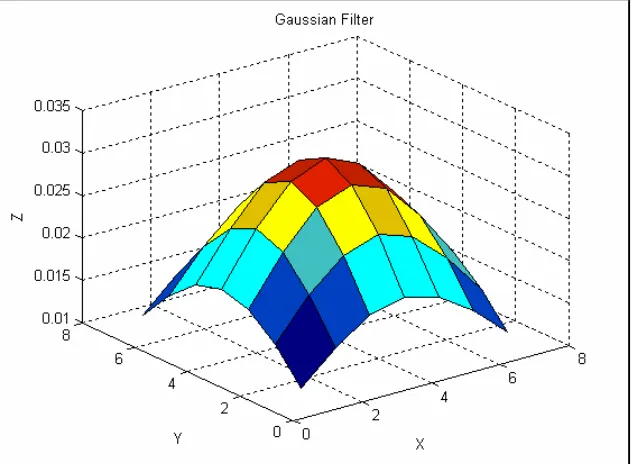
2.3.5 Gaussian Smoothing

When the Gaussian filter is convolved with an image, it removes the noise from the image but also blurs the image and removes the details from it. It is a ‘low pass filter’. In working it is similar to an averaging filter. But the mask used in Gaussian smoothing is different from the mask used in an averaging filter. The mask used for Gaussian

(19)

The Gaussian filter can be specified by the user by providing the mean and standard deviation.

2D circularly symmetric Gaussian has following form [32]

2 2 2

2 2

2

1

)

,

(

σ

πσ

y x

e

y

x

G

+ −

=

In this work Gaussian filter of size 7*7 and standard deviation of 3 is used for smoothing the frames before finding interesting features in it. This Gaussian filter is shown in the fig [2] and is generated by the following code snippet in Matlab.

w = fspecial(‘gaussian’, 7, 3);

surf(w), title('Gaussian Filter used for Smoothing'), xlabel('x'), ylabel('y'), zlabel('z');

In OpenCV this filter is generated by using following code snippet

cvSmooth(imgSrc, imgDst, CV_GAUSSIAN, 7, 7, 3);

[image:19.612.149.465.438.670.2]

Where ‘imgSrc’ is the source image and ‘imgDest’ is the destination image. Both images can have either 1 or 3 channels and can have either 8 bit or 32 bit floating point values.

(20)

[image:20.612.93.524.154.384.2]

Applying Gaussian smoothing before edge detection can be useful since it softens the edges and filters out the noise in an image. Using a small Gaussian filter, e.g., of size 3*3 or 5*5 will give fine details but it will also give many unwanted edges due to noise and fine texture. A large smoothing filter may remove most of the unwanted edges but much of the details might also be lost [13].

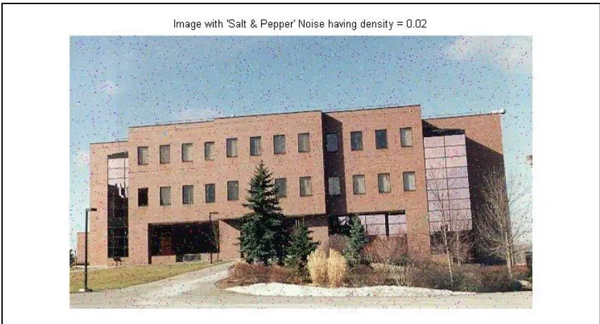
Figure 3. Original Image ‘CIS_Building.jpg’. Taken from [31].

(21)

[image:21.612.89.523.70.304.2]

Figure 4. After adding ‘Salt & Pepper’ noise with density = 0.02 to fig [3].

To get rid off the noise the image is smoothed with the Gaussian filter, shown in fig [2], and the resulting image is fig [5].

[image:21.612.92.525.396.637.2]

(22)

2.3.6 Feature Point Extraction

In this work, the video can be taken either from a moving camera or a stationary camera. For a video taken with a panning camera two consecutive frames of that video can give the information about the relative velocity of the camera. The amount by which each pixel in the current frame is shifted from the previous one can be computed and the mode of the shift values in the x and y directions of all the pixels in current frame can be computed to obtain the shift introduced by the movement of the camera. But comparing every pixel in the current frame with all the pixels within certain neighborhood of the previous frame is computationally very expensive. Hence in this work only feature points (corners) found in the current frame are mapped to their corresponding feature points in the previous frame and the shift in their spatial coordinates is found and the current frame is adjusted for that amount of the shift. This reduces the time complexity of the algorithm [29].

Feature point extraction involves finding interesting points in an image. In this work interesting points are found on the previous frame, ft-1, and the current frame, ft.

Any typical indoor or outdoor video taken from either a stationary or moving camera will have objects on background and moving foreground objects. For e.g. a car moving on the road contains the moving car as the foreground objects and road or trees or houses in the background. So for a video taken with a panning camera both the background and foreground objects will be in relative motion. After finding the amount and direction of the shift in the static background objects the relative velocity of the moving camera can be estimated. Hence by focusing only on the objects in the video the shift in the camera can be obtained. Objects in an image can be highlighted by finding the edges in the image since edges represents boundaries of the object in the image. For the objects having different color than the background, the edge corresponds to the boundary between the object and the background or different part of the same object. Hence an edge indicates a sudden jump in intensity from one pixel to another pixel in the direction perpendicular to the edge. Hence an edge indicates a sharp contrast in the intensity [14].

Detecting edges in an image is most common approach of finding meaningful

discontinuities in an image rather than detecting points and lines in an image. To detect edges in an image, discontinuity in intensity values need to be detected by the first order and the second order derivatives of the image, as derivatives gives rate of change of the some quantity.

Derivatives of an image are explained in detail in [15]. The following paragraphs summarize the work in [15] and the formulas are taken from [15].

Derivatives are required to find the sudden changes in the image intensity indicating edges or corners. But OpenCV or Matlab treats an image like a 2D or 3D array of pixels, i.e., a grayscale image I of size width*height is an array I of width columns and height

(23)

derivatives can be found only for the continuous functions. Hence for the purpose of derivations, image is considered to be sampling of a continuous function of the variables x and y [15].

A vertical edge in the image indicates a sharp contrast in the intensity in the horizontal direction i.e. the direction perpendicular to it. Vertical edges in the image can be found by taking the derivative of the image in the horizontal direction. Hence while taking the derivative of the image with respect to x axis i.e. the horizontal axis any derivative with a very high positive or negative value indicates a vertical edge at that x coordinate [15].

For a continuous function f(x, y) its partial derivative with respect to x axis is given by

x y x f y x x f x y x f x ∆ − ∆ + = ∂ ∂ → ∆ ) , ( ) , ( lim ) , ( 0

where ∆xis an arbitrarily small value [15]. But if f(x, y) is a discrete function

representing a 2D digital image then the value of ∆xis 1 pixel which is the smallest in the image. Hence the derivative of the image at location (i, j) is given by [15]

) , ( ) 1 , ( ) , ( j i f j i f x y x f − + ≈ ∂ ∂

Where j=x and i=y.

This is same as convolving the image with the mask of [1 -1].

Hence the first derivative of image can be found by convolving it with the following masks

1. [1 -1] to find derivative with respect to horizontal i.e. x direction.

2. _      −1 1

to find derivative with respect to vertical i.e. y direction

The other variant of the filters used are

1. [1 0 -1] to find derivative with respect to horizontal i.e. x direction.

2.           −1 0 1

Similarly the 2nd order derivative of the image can be found by convolving the image with following filters or masks

(24)

2.

  

 

  

  −

1 2 1

Since and edge indicates the change in intensity its 1st and 2nd derivative indicates the amount and direction of this change.

Figure 6. Figure indicating the 1st and 2nd derivative of an edge. Taken from [10].

The two most common approaches to find the 1st and 2nd derivatives of the image are

Prewitt compass edge detection and gradient edge detection.

In Prewitt edge detection the image is convolved by a set of eight masks, each of which is sensitive to a different edge orientation. The mask which produces the maximum

response determines the magnitude and direction of the edge. Different types of masks are Sobel, Prewitt, Roberts etc.

(25)

The concept of edge detection using gradient is explained in detail in [9]. The following formulas for gradient are taken from [9].

For a 2D function, f(x, y), its gradient is defined as the vector [9]

            ∂ ∂∂ ∂ =       = ∇ y f x f G G f y x

The magnitude of this vector is given by [9]

[

]

              ∂ ∂ +       ∂ ∂ = + = ∇ 2 2 2 / 1 2 2 y f x f G G f _x _y

It is often approximated by [9]

y

x G

G

f ≈ +

∇

“The gradient vector points in the direction of the maximum rate of change of the function f at coordinates (x, y) and the angle at which this maximum rate of change occurs is given by” [9]

      = − x y G G y

x, ) tan 1 (

α

The horizontal gradient, Gx, at a pixel can be found by convolving it with the mask

[-1 0 1] andthe vertical gradient at a pixel can be found by convolving it with the mask [1 0 -1]T.

In this work corners are used as interesting points. It is assumed that most of the corners found in the previous frame, ft-1, would be preserved in the current frame, ft. Few of the

corners found in the previous frame might be out of view in the current frame due to the motion of the camera. But most of the corners found in the previous frame will be still found in the current frame, but they might be shifted by certain amount depending upon the motion of the camera.

(26)

[image:26.612.94.524.426.669.2]

The corners detected on the noisy image in fig [4] are shown below in fig [7].

Figure 7. Corners detected on the image in fig [4].

The corners detected on the image, which is obtained after smoothing the noisy image (fig [5]), are shown in fig [8].

(27)

The number of false corners detected, after smoothing the image with Gaussian filter, is much fewer as compared to the false corner detected in the noisy image without

smoothing. For example, in fig [8] the corners in the trees, glass window wall on right side and sky are much fewer as compared to the corners in fig [7].

But since smoothing causes blurring of the image, the number of the true corners detected after smoothing the image also decreases. For example, there are fewer true corners around the window glasses.

But in this work, the frames are smoothed before finding the corners because the

reduction in the number of the true corners caused after smoothing the frame isn’t drastic. There are still enough true corners to do frame registration. Also after smoothing, the false corners caused due to noise are removed and hence the chance of getting better registration increases.

There are many corner detectors. But this work uses Harris Corner Detector. Since the corners are formed by intersection of two or more edges and edges usually define the boundary between two different objects or parts of same object, they are interesting.

A detailed comparison of all the corner detectors can be found in [29]. This work summarizes most common corner detectors and is based on [29].

Most of the corner detectors have the same general algorithm having following steps

1. Applying Corner Operator to Obtain Cornerness map: All the corner detectors have some type of corner operator which assigns a cornerness value to every pixel in an image. Cornerness value is measure which indicates how well a pixel represents a corner. The corner operator is a main differentiating factor between different corner detectors. A cornerness map gives the cornerness measure of every pixel in the input image and hence has the same dimension as that of the input image.

2. Thresholding Cornerness Map: From the Cornerness map obtained in step 1, pixels with the local maximum cornerness values have chances to represent a corner. But there might be many pixels which are local maximum but their cornerness value is too small to represent a corner. Hence a threshold is required to avoid detection of local maximum pixels with low cornerness values as corners. Threshold value is application dependent.

(28)

The most common corner detectors are

1. Moravec Corner Detector: Moravec operator defines a point having large intensity variations in all the eight principle directions (left, right, top, bottom, top-left, top-right, bottom-right and bottom-left) as an interesting point. Since this property is similar to that of the corner, Moravec operator is considered to be the corner detector.

For every pixel I(x, y) at location (x, y) in an image, Moravec Operator finds intensity variation at that pixel in by

1. Placing a square window (typically of size 3*3, 5*5 or 7*7) centered at (x, y) and shifting that window by one pixel in each of the eight principle directions.

2. For a particular shift intensity variation is calculated as the sum of the square of the intensity differences between the corresponding pixels in these two windows (shifted window and the original window centered at (x, y)).

3. After finding the intensity variation for each of the eight shifts the minimum intensity variation is selected as the intensity variation at location (x, y).

Mathematical notations of Moravec Operator can be given by

2 , ,

, ,

, x u y v uv v

u v u y

x

w

I

E

=

∑

₊ ₊

−

Where w is the image window having the value 1 in the specified rectangular region and 0 elsewhere. x and y are the shifts in 8 principle directions having value (1, 0), (-1, 0), (0, 1), (0, -1), (1, 1), (1, -1), (-1, 1) and (-1, -1).

There are four cases that needs to be considered while using Moravec Operator

1. If the portion of the image under the window is of constant intensity, then all the shifts will result in negligible intensity change.

2. If the window is along the edge, then any shift along the edge results in small change but any shift perpendicular to the edge results in significant changes.

3. If the window is on the isolated point then all the shifts will result in large change.

(29)

The Moravec Corner detector has following drawbacks

1. Since the shifts in only eight principle directions, i.e., at every 45 degrees is considered the response of the operator is very anisotropic.

2. Since the window considered is rectangular and binary the response is noisy.

3. Since the minimum intensity variation out of all the shifts is taken into account, it detects corners all along the diagonal edges which don’t lie parallel to the eight principle directions. Hence the Moravec operator is not rotation invariant. If the image is rotated and after rotation most of its edges are not parallel to the eight principle directions then the number of corners found will be too large.

A detailed explanation of Moravec operator and its drawbacks is given in [29].

2. Harris/Plessey Corner Detector: Harris corner detector overcomes many drawbacks of the Moravec Corner detector.

1. Moravec corner detector was anisotropic since it considered shifts at every 45 degrees. Harris corner detector removes this drawback by performing intensity variation measurement at all possible small shifts. The change E produced by any arbitrary shift (x, y) is given by

2 , , ,













∂

+

∂

=

∑

y

I

y

x

I

x

w

E

v u v u y x Where x I ∂ ∂

= I ⊗[-1 0 1] and

y I

∂ ∂

= I ⊗[-1 0 1]T and ⊗ is convolution operator.

For (x,y) having values (1, 0), (-1, 0), (0, 1), (0, -1), (1, 1), (1, -1), (-1, 1) and (-1, -1) it behaves approximately like Moravec Corner Detector.

This new measure of intensity variation can measure intensity changes in all possible directions by proper selection of x and y values.

(30)

Figure 9. Method of computing value of x and y. Taken from [29]

2. Moravec Operator uses rectangular and binary window. Since the window

is square all the pixels in corner of the square are not equidistant from the center. Harris corner detector uses a circular window so the Euclidean distance from the center pixel of the window to the edge of the window is same in all the directions and hence gives better measurement of the local intensity variation. Also window in Moravec operator is binary, i.e., it assigns equal weights to all the pixels in the window. But the pixels near the center of the window are better indicator of the local intensity variations as compared to the pixels on the edges of the window. So pixels near the center of the window should be given the higher weight.

Hence the Harris corner detector uses a circular Gaussian window given by

(

)

2 2 2 2 , σ v u v u

e

w

+ −

=

3. Moravec operator detects many corners along the edges which are not parallel to any of the eight principle directions.

“Any imperfections in an edge due to intensity quantization, pixilation or noise may result in the increase of the minimum local intensity variation”. [29]. Harris corner detector overcomes this drawback by reformulating it in the following way (Derivation taken from [29]).

(31)

=

              ∂ ∂ + ∂ ∂ ∂ ∂ +       ∂ ∂

∑

2 2

2 2 , , 2 Y I y y I x I xy x I x w v u v u

=

2 2

2Cxy By

Ax + +

Where A = 2       ∂ ∂ x I

⊗w, B = 2       ∂ ∂ y I

⊗w and C = _

     ∂ ∂ ∂ ∂ y I x I ⊗w

They further represent the equation as

E

x,y

=

Ax2 +2Cxy+By2

=

[

]

_      y x M y x

Where _

     = B C C A

M [29].

Reformulated cornerness measure considers the variation between the intensity changes in different direction.

If the 2D image is visualized as a 3D surface where x and y coordinates of the image are the two dimensions and the 3rd dimension is the pixel intensity, then the matrix M contains all the differential operators describing the image surface at a given point (x, y).

(32)

Figure 10. Eigenvalues indicating the principle curvature of the image surface. Taken from [29].

There are three different cases to be considered

1. For the portion of the image within the window having relatively constant intensity, there is little curvature and hence both the eigenvalues are relatively small, which indicates there is no corner. 2. For the window along the edge, there is a very less curvature along the

edge and a very high curvature perpendicular to the edge i.e. one curvature is high and another curvature is low forming a ridge indicating the edge.

3. For corner and isolated point both the curvature will be high so both eigenvalues would be high.

To obtain the cornerness map, Harris corner detector uses the following cornerness measures [29]

B A M trace C AB M M trace k M y x C + = + = − = = − = 2 1 2 2 1 2 ) ( ) det( )) ( ( ) det( ) , (

λ

(33)

Algorithm for Harris Corner Detector

1. For each pixel at coordinate (x, y) in the image compute the autocorrelation matrix M.

2. Compute the cornerness measure C(x, y) and create the cornerness map.

3. Set all the points in cornerness map having cornerness measure less than the threshold to 0, i.e., if C(x,y) < threshold then C(x, y) = 0. 4. Use non-maximal suppression to find local maxima.

In this work, Gaussian smoothing was performed before using Harris Corner Detector to get rid of noises.

In this work, OpenCV [30] function cvGoodFeaturesToTrack() is used to determine strong corners in image. cvGoodFeaturesToTrack() has a parameter which if set to non-zero uses Harris Corner Detector to detect corner and if set to non-zero then finds corner with large eigen values in an image.

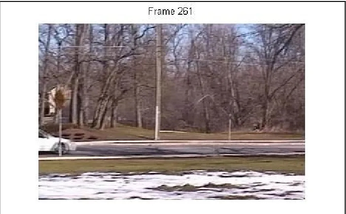
[image:33.612.130.483.361.584.2]

Below are the two consecutive frame, frame 260 and frame 261, which are taken from a video ‘car_pan.avi’. The video was taken from [31].

(34)

[image:34.612.131.482.71.289.2]

Figure 12. Frame 261 of video ‘car_pan.avi’

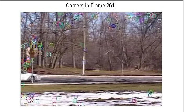
After finding corners in the above two frames the resulting frames are shown in following figures, fig[13] and fig[14].

(35)

[image:35.612.131.483.72.286.2]

Figure 14. Corners found in Frame 261.

2.3.7 Correspondence Measures

After finding the interesting points, i.e., the corners in two consecutive frames, all the feature points in the previous frame, ft-1, must be matched with their corresponding

feature points in the current frame, ft. The general method of finding correspondence is,

compare every feature point, P(x, y), in the previous frame, ft-1, with all feature points in

the current frame, ft,in certain N*N neighborhood of location (x, y), where N is the

maximum amount of shift which can be caused by camera in two consecutive frame. In this work the value of N is assumed to be 20, i.e., it is assumed that camera wouldn’t pan fast enough to cause a shift in pixel in two consecutive frames by amount more than 20 in any given direction.

To compare a feature point P1(x, y) (pixel at location (x, y)) in the frame ft-1 with a

feature point P2(x’, y’) in the frame ft, usually their intensity values are not compared

directly because it can be error prone due to noise effects. Instead a square window, w1, of certain size (for e.g. 3*3, 5*5 or 7*7 etc) centered at P1(x, y) and another square window, w2, of same size centered around P2(x’, y’) are compared. The distance between these square windows, w1and w2, is found. This distance is measure of how close these two pixels P1(x, y) and P2(x’,y’) are.

The most common method of finding the distance between these two windows is sum of squared difference between corresponding intensities.

(36)

Intensity Matrix (I1) Intensity Matrix(I2) 55 A1 31 A2 44 A3 53 A4 37 A5 45 A6 45 A7 38 A8 51 A9

The Sum Squared Distance in given by

SSD =

2

9 1 ) ( _i i i B A −

∑

=

But in this work the correspondence measure used to match the feature points in two consecutive frames is taken from [8]. It is called Ordinal Measures.

According to the Ordinal Measures, to compare two corners for similarity, instead of directly comparing their N*N neighborhood of the intensity plane, the pixels in their N*N neighborhoods are ranked according to their intensity to get a rank matrix of dimension N*N and instead of the N*N intensity matrices those N*N rank matrices are compared. They also propose a measure to find the distance between the two rank matrices. This makes the correspondence measure invariant to changes in illumination caused by shadows, sun light or any light in indoor scenes.

It is based on the idea that any change in intensity caused due to shadows, sun light or any other indoor light will probably effect not only the pixel but also its small N*N neighborhood equally. So the pixels in the N*N window should preserve their ranks. Hence, instead of comparing the intensity matrices directly, the intensity matrices are converted to rank matrices and the rank matrices are compared.

For example, the intensity matrix and its corresponding rank matrix for the pixels in 3*3 neighborhood of a corner are

Intensity Matrix Rank Matrix

17 33 75

24 52 87

41 68 94

They also define a measure to find distance between the two rank matrices, i.e., how close the 2 rank matrices are. Let I1 and I2 be two N*N intensity matrices. The

corresponding N*N rank matrices are

π

1 and

π

2. They define a composition permutation, S, as follows

55 B1 31 B2 44 B3 53 B4 37 B5 45 B6 45 B7 38 B8 51 B9

1 3 7

2 5 8

(37)

Si =

π

₂k

k= (

π

₁−1)i

Where i = 1 to N*N. 1 1

−

π

denotes the inverse permutation of

π

1. They define the inverse

permutation as: if i

1

π

= j, then ( 1 1

−

π

) j = i. Hence Si is the rank of the pixel in I2 that

corresponds to the pixel with rank i in I1. Under perfect correlation, S, should be identical

to the identity permutation given by U = {1, 2, 3… n*n}.

Then they define a distance measure between S and U which in turn gives the distance measure between

π

1 and

π

2. They define deviation dmi at each S

i

as the number of Sj, j = 1,…,i greater than i

i m d

=

∑

= > i j i J 1 j ) S (

= i -

∑

= ≤ i j i J 1 j ) S (

Where J(B) = 1 when B is true and 0 otherwise.

The vector d_mi is termed as distance vector dm (s, u). It estimates the number of S

elements that are out of position. If I1 and I2 were perfectly correlated, then dm (s, u) = (0,

0, …., 0). The maximum value that any component of the distance vector can take is

    2 n

which occurs in the case of perfect negative correlation.

Then they define a measure of correlation

κ

=

κ

( I1, I2) as

κ

( I1, I2) = 1 -

    = 2 max 2 1 n dmi n i

If I1 and I2 were perfectly correlated then

κ

=1 and

κ

=-1 when they are perfectly

uncorrelated.

For example, for a pixel intensity matrix I1 in the frame ft-1 and intensity matrix I2 in the

(38)

I1 I2

29 38 47

61 42 58

39 71 44

π

1

π

2

1 2 6

8 4 7

3 9 5

Therefore

π

1 = {1, 2, 6, 8, 4, 7, 3, 9, 5} and

π

2 = {1, 3, 4, 7, 5, 8, 9, 2, 6}

π

11 = 1,

π

1-1 = 1,

π

21 = 1, S1= 1

π

12 = 2,

π

1-2 = 2,

π

22 = 3, S2= 3

π

17 = 3,

π

1-3 = 7,

π

27 = 9, S3= 9

π

15 = 4,

π

1-4 = 5,

π

25 = 5, S4= 5

π

19 = 5,

π

1-5 = 9,

π

29 = 6, S5= 6

π

13 = 6,

π

1-6 = 3,

π

23 = 4, S6= 4

π

16 = 7,

π

1-7 = 6,

π

26 = 8, S7= 8

π

14 = 8,

π

1-8 = 4,

π

24 = 7, S8= 7

π

18 = 9,

π

1-9 = 8,

π

28 = 2, S9= 2

S = {1, 3, 9, 5, 6, 4, 8, 7, 2}

dm1 = 1 – J(S1≤1) = 1 – 1 = 0

dm2 = 2 – [ J(S1≤2) + J(S2≤2)] = 2 – [1+0] = 1

dm3 = 3 – [ J(S1≤3) + J(S2≤3) + J(S3≤3)] = 3 – [1+1+0] = 1

dm4 = 4 – [ J(S1≤4) + J(S2≤4) + J(S3≤4) + J(S4≤4)] = 4 – [1+1+0+0] = 2

dm5 = 5 – [ J(S1≤5) + J(S2≤5) + J(S3≤5) + J(S4≤5) + J(S5≤5)]

= 5 – [1+1+0+1+0] = 2

dm6 = 6 – [ J(S1≤6) + J(S2≤6) + J(S3≤6) + J(S4≤6) + J(S5≤6) + J(S6≤6)]

= 6 – [1+1+0+1+1+1] = 1

dm7 = 7 – [ J(S1≤7) + J(S2≤7) + J(S3≤7) + J(S4≤7) + J(S5≤7) + J(S6≤7) +

J(S7≤7)] = 7 – [1+1+0+1+1+1+0] = 2

dm8 = 8 – [ J(S1≤8) + J(S2≤8) + J(S3≤8) + J(S4≤8) + J(S5≤8) + J(S6≤8) +

J(S7≤8)] = 8 – [1+1+0+1+1+1+1+1] = 1

dm9 = 9 – [ J(S1≤9) + J(S2≤9) + J(S3≤9) + J(S4≤9) + J(S5≤9) + J(S6≤9) +

J(S7≤9)] = 9 – [1+1+1+1+1+1+1+1+1] = 0

33 42 44

59 47 62

68 37 54

1 3 4

7 5 8

(39)

dm = {0, 1, 1, 2, 2, 1, 2, 1, 0}

κ

( I1, I2) = 1 -

    2 9 2 * 2 = 0 2.3.8 Transformations

To summarize, in the previous sections interesting points are found in the current frame and the previous frame and after that they are matched according to ordinal measures. After matching the feature points the amount by which each of them are spatially shifted is found and the mode of all the shifts gives the amount and direction of the shift

introduced by the moving camera. To find the pixels on the silhouettes of moving foreground objects, the current frame needs to be shifted in the direction and by the amount of the shift introduced by the panning camera. Hence a proper transformation is needed to align the current frame according to the previous frame.

In this work the source of misregistration is the panning camera and hence a proper transformation should be selected to remove the spatial distortions.

The main transformations are rigid, affine, projective, perspective and polynomial.

The rigid transformation can be used for registering the images having distortions introduced either due to translation or reflection. It maintains the relative shape and size of the objects in the reference and target images. It involves recognition of same objects in the reference and target images and finding their coordinates. After finding this

information cross-correlation is applied and then through some image manipulation input images are either overlaid or expanded to get a larger output images.

Affine transformations maintain collinearity, i.e., all points lying on a line initially still lay on a line after transformation, and the ratios of distances, for example, midpoint of line segment remains the mid point after transformation. Affine transforms are most commonly used transformation since they are sufficient to match two images taken from same viewing angle but different position. Affine transformation consists of the Cartesian operations of a scaling, a translation and a rotation. It does not change the overall geometric relationships between the points. It does not necessarily preserve angles or lengths [6].

An affine transform has typically four parameters tx, ty, sand θ which map a point (x1, y1)

of the first image to a point (x2, y2) of the second image according to the following

formula (equation taken from [4])

      2 2 y x

=

_      y x t t

+

s*

_

(40)

For registration of the images involving other spatial distortions like skew and aspect rations the general 2D affine transform used is (equations taken from [4])

      2 2 y x

=

_      23 13 a a

+

_      22 21 12 11 a a a a       1 1 y x

The perspective transformations are used when the images to be registered has distortions introduced due to projection of 3D scene onto a 2D plane. Due to projective distortions the objects which are father away from the camera appear smaller and the objects which are more inclined away from the camera appear to be more compressed [4]. The mapping between the coordinates of object in 3D world, (x, y, z), and the corresponding coordinates (x’, y’), in 2D image is given by (Equations taken from [4])

x’ =

f z

fx

− −

y’ =

f z

fy

− −

where f is the focal length of the camera.

The rectification transformation is used in registering a scene tilted with respect to image plane to a tilt free target image of desired scale.

Complicated differences between reference and target images like different positions, different angels and shearing can be handled by affine transformation by mapping straight lines from two separate images. But the moving foreground object extraction algorithm in this work takes into account only the translation, because for any two consecutive frames shearing and rotation doesn’t have significant effect and implementing it would be computationally expensive. Simple translation is used to correct the current frame after interesting features in current and previous frames have been matched.

2.4 Algorithm used for Background Subtraction in this Work

For finding correspondence between two consecutive frames, ft-1 and ft, first the corners

are found in the frames ft-1 and ft and then for every corner, (x, y), in ft-1 its

corresponding corner, (x’, y’), in the frame ft is found by comparing the 11*11 rank

matrix of the corner, (x,y), in ft-1 with 11*11 rank matrix of every corner in 41*41

neighborhood of (x, y) in ft, i.e., rank matrix of all the corners in frame ft in the range

(x-20 to x+(x-20, y-(x-20 to y+(x-20) are compared with rank matrix of the corner (x, y) in frame ft-1

and the most matching point is declared as the corresponding point of corner (x, y).

After matching a corner point P1(x, y) in ft-1 with corner point P1(x’, y’) in ft the amount

(41)

This shift is found for all the corners in ft-1. After the shift in x and y direction for all the

corner points in the frame ft-1 is found, the mode for all the shifts in x and y direction is

found and that gives the net shift in x and y direction caused by panning of the camera.

The frame, ft,is shifted by that much amount.

After shifting the frame ft,a simple difference between the frame ft-1 and ft gives the

difference image which contains just the pixels (mostly on silhouette’s) of the moving objects.

[image:41.612.105.509.233.542.2]

Algorithm for finding moving foreground objects

Figure 15. Block Diagram of Algorithm for finding pixels on moving foreground objects.

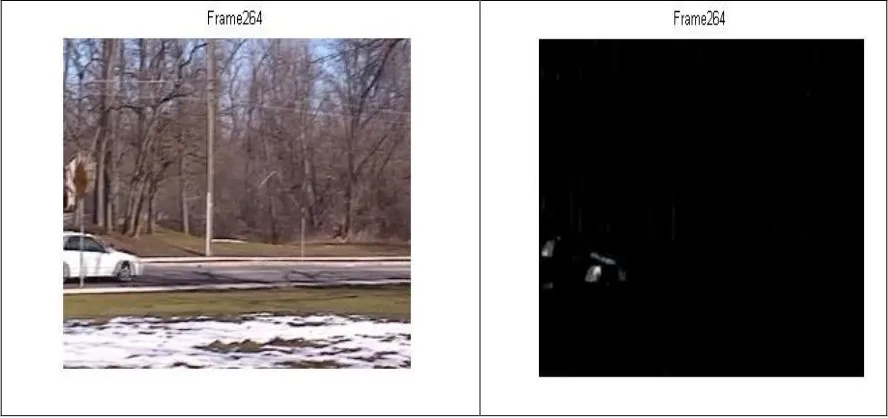
2.5Results after Subtracting Background

The frames from 258 to 264 are shown below. During these frames the camera is panning towards right and the car is also moving towards right. The original frames are of the size 340*260 but have been scaled down for proper display. The frames from original

‘car_pan.avi’ video are shown in the 1st column and in the 2nd column the frames containing only the moving foreground objects (i.e. is only the car) are shown. Most of the pixels belong to the silhouettes of the moving object.

START

Take two consecutive frames of the video, ft and ft-1.

Find interesting points in the frames, ft and ft-1,using Harris corner detector.

Establish correspondence between interesting points in frames ft and ft-1using

ordinal measures.

Find the amount by which the frame ft is shifted and correct the ft for that much

shift. Subtract the frame ft from ft-1.

(42)

(43)

(44)

[image:44.612.84.528.72.281.2]

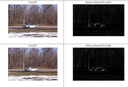
Figure 16. Results for Background Subtraction performed on the Video Taken from a Panning Camera.

The results for the videos taken from the stationary camera are also shown below.

The frames from 140 to 148 of the video ‘Elephant.avi’ (taken from [31]) are shown in 1st column. Only the elephant is the moving foreground object. Also the camera isn’t

panning.

(45)

(46)

(47)

[image:47.612.88.527.71.295.2]

(48)

3 Object Segmentation and Related Work

3.1 Object Segmentation

From the previous section, after adjusting the current frame ft, to correct for the motion

introduce by panning of the camera, and subtracting it from the previous frame ft-1, we

get the pixels on the silhouette’s of the moving foreground objects. The output of this stage is just the pixels on the silhouettes of moving objects. However the system doesn’t know which group of pixels represents a single logical object. So the next step is to incorporate intelligence in the system so that it knows which groups of moving pixels are parts of a single logical object. For example, in a scene containing many moving cars there would be moving pixels on the front and back portion of every car and also a few pixels on the other boundaries of the cars. But the system should be able to tell which groups of moving pixels belong to which car.

Hence an ideal object segmentation system should be able to identify semantically meaningful components of the image and should be able to group the pixels belonging to such components.

A very detailed survey about different object segmentation techniques is given in [17]. Following sections summarize most of the relevant work given in [17].

3.2 Related Work

The main methods for segmenting moving objects are

1. Spatial Segmentation.

2. Motion based Segmentation.

Any monochrome image has two types of information: spatial information and intensity information. Spatial information gives the location of a pixel in the 2D image and

intensity information gives the intensity or graylevel value of that pixel. The combination of the spatial and intensity information for regions of pixels defines the various features of an image like edges, corner, shapes etc. A video is a sequence of images collected at a certain interval of time. Examining a sequence of images yields a third type of

information known as temporal information which can be defined as a combination of spatial and intensity information as a function of time. This work uses Spatio temporal information along with motion based information to segment moving objects.

3.2.1 Spatial Segmentation

The methods in this category directly manipulate the pixel intensities in the image plane or spatial domain of the current video frame to segment the objects. They don’t use any temporal or motion information.

(49)

1. Region Based

2. Contour Based.

These methods are not very successful since they don’t use temporal and motion based information present in sequence of frames of a video.

Figure 18 Classification of Spatial Segmentation Methods. Taken from [17].

3.2.1.1 Region Based Method

The commonly used region based methods for object segmentation are

1. Color segmentation

2. Histogram segmentation and

3. Region Growing.

This section provides the overview of these three methods

1. Color Segmentation: Color segmentation is used to segment objects of specified color range from the input image. The range of colors to be segmented is

specified and the algorithm iterates through each pixel in the input image to determine whether the pixel belongs to specified color ranges or not. Euclidean distance or Mahalanobis distance is used to find the distance between the color of the pixel and the desired color. More details about color segmentation are given in [9].

But this is a very naive method for segmentation and not very useful. It is not possible to specify the ranges of the colors of all moving objects. Color composition for many moving objects cannot be predicted in advance. For

Spatial Segmentation Methods

Region Based Segmentation Contour Based Segmentation

Region Growing

Color Segmentation

Histogram Segmentation

Edge Detection Contour

(50)

example a person might wear different color clothes on different days so it is difficult to predict the color of object in an image. Also many background and foreground objects may have the same color. In this case the background objects will also be classified as foreground objects.

So the color segmentation based methods are rarely used alone for segmenting moving objects. They are usually combined with motion based segmentation or edge detection.

2. Histogram Segmentation: Histogram is a graphical way of displaying the table which shows what proportion of cases fall into each of the several specified categories. In [28] histogram based segmentation is used. In [28] motion mask is obtained by using frame differencing, after correcting the frame for the motion of the camera. The motion mask obtained after subtracting the current frame from the previous frame generally contains the pixels on the silhouette of the moving objects. This motion mask is anded with the original frame to give the color of the deformable moving objects and along with it some portion of the background too. The histogram of the intensity value of the pixels obtained from anding mask and frame is then constructed. The threshold is applied to the histogram to get the most frequently occurring colors and the objects in the current frame with those particular ranges of colors are highlighted. But this method has few drawbacks. Coming up with a generic threshold for all the videos is difficult. If the threshold is not appropriate then this method may grab a considerable amount of

background. Also if the moving object is of the same color as the stationary object then the stationary object will also be segmented. For example, if there are two polar bears of white color in the video and one is moving and the other is not, this method will segment both the moving as well as non-moving polar bears. This method doesn’t take advantage of the motion information which can be obtained from the sequence of video frames.

(51)

3.2.1.2 Contour Based Segmentation

1. Edge Detection: Different edge detectors like Sobel or Canny edge detectors are used to find edges in the image. They are then used in combination with region growing to restrict the over-segmentation resulting from region growing.

2. Contour Detection: Closed contours are detected after detecting the edges in the image. The region within the closed contour is region grown with the region growing algorithm.

3.2.2 Motion Segmentation

The techniques in motion based segmentation falls into 2 groups depending upon the dimensions of the motion models used for segmentation. These groups are

1. 2D Approach and

2. 3D