Exploring the Kinetics of Domain Switching in Ferroelectrics for Structural Applications

(1)

Exploring the Kinetics of Domain Switching in

Ferroelectrics for Structural Applications

Thesis by

Charles Stanley Wojnar

In Partial Fulfillment of the Requirements for the Degree of

Doctor of Philosophy

California Institute of Technology Pasadena, California

2015

(2)

c 2015

(3)

(4)

Acknowledgments

First and foremost, I acknowledge Professor Dennis Kochmann, my Ph.D. research advisor, from whom I have learned to always do the best I can and put as much effort as I can into everything I do, not only in research but also in my life. He is the best example of a great researcher, teacher, and mentor and is an example I hope to emulate in my future career. I thank my committee members. Professors Kaushik Bhattacharya and Ravi Ravichandran were generous enough to let me attend their group meetings (and eat their food) even though I was not in either of their groups. The meetings were always intellectually stimulating for me and I have learned a lot from my interactions with Kaushik and Ravi and their students, in particular Mike Rauls, Srivatsan Hulikal, Cindy Wang, Mauricio Ponga, Zubaer Hossain, Vinamra Agrawal, Jacob Notbohm, Gal Shmuel, and Bharat Penmecha. The meetings were also a great opportunity for me to get feedback on the work I was doing from my peers. Kaushik and Ravi have also been great resources for me as I went through my job application process. I am also grateful for Professor Pellegrino for serving on my committee. I have benefited tremendously from my interactions with his students, who have helped me get started with my experiments, namely Keith Patterson and John Steeves.

I wish to express my gratitude to Professor Ioannis Chasiotis, my undergraduate advisor, whose encouragement convinced me to apply to GALCIT for graduate school, even when I doubted myself. My decision to apply and later come here was the best decision I have made in my life. I have learned so much and have made so many great friends at Caltech. I would also like to thank Nikhil Karanjgaokar, who was my graduate mentor when I was working in Ioannis’ lab as an undergraduate and who has continued to provide guidance and encouragement to me since he has come to Caltech as a postdoc.

(5)

Amelang is one of the nicest people I know and his great teaching abilities have inspired me to strive to improve my own. I wish to acknowledge Jean-Briac le Graverend, a great experimentalist, from whom I have learned so much and have received so much encouragement during his time in the group. Possibly the most important thing was that he helped me improve my golf game! I also wish to express my appreciation for everyone else in the group (and former members): Benjamin Klusemann, Neel Nadkarni, Ishan Tembhekar, Gabriela Venturini, and Alex Zelhofer.

There were many people from other groups at Caltech and elsewhere who were kind enough to take the time to help me with various aspects of my research. I thank Professor Sossina Haile and her student Chris Kucharczyk for training me and letting me use their equipment. Similarly, I thank Professor Julia Greer (whom I particularly thank for serving on my committee during my candidacy exam) and her students, Zach Aitken, Lucas Meza, and Lauren Montemayor for their help and for letting me use some of their equipment. I thank the students of Professor Ortiz, who have helped me through my many mathematical shortcomings. In particular, I am thankful for the help of Jonathan Chiang and Brandon Runnels. I am grateful for my interactions with Professor Chris Lynch and several of his students at UCLA. I could not have started my experiments without their guidance. I am glad to have the opportunity to work with Case Bradford at JPL. Through our collaborations I was actually able to see potential applications for my work.

I have had such a great experience being a part of the GALCIT family and have had great interactions with not only fellow students and faculty, but also staff. In particular, I would like to mention Denise Ruiz, who was one of the few people I could go to at Caltech to talk about something besides science. She continually exhibited professionalism in everything she did, even under the most demanding circumstances (such as when I screwed up my travel expenses). I also thank Francisco who was always willing to take the time to talk to me about anything that was on my mind. I am thankful for the lab support from Petros Arakelian and the machine shop staff, Joe, Brad, and Ali. Finally, I am extremely glad to have come to GALCIT with my fellow first-year students and would not have made it this far without their friendship and assistance on coursework: Neal Bitter, Peter Bridi, Subrahmanyam Duvvuri, Esteban Hufstedler, Cheikh Mbengue, Stephanie Mitchell, Nisha Mohan, Lauren Montemayor, Gina Olsen, Karen Oren, Vishagan Ratnaswamy, John Steeves, Dustin Summy, and Yuan Xuan.

(6)

Abstract

The complex domain structure in ferroelectrics gives rise to electromechanical coupling, and its evolution (via domain switching) results in a time-dependent (i.e. viscoelastic) response. Although ferroelectrics are used in many technological applications, most do not attempt to exploit the viscoelastic response of ferroelectrics, mainly due to a lack of understanding and accurate models for their description and prediction. Thus, the aim of this thesis research is to gain better understanding of the influence of domain evolution in ferroelectrics on their dynamic mechanical response.

There have been few studies on the viscoelastic properties of ferroelectrics, mainly due to a lack of experimental methods. Therefore, an apparatus and method called Broadband Electromechanical Spectroscopy (BES) was designed and built. BES allows for the simultaneous application of dynamic mechanical and electrical loading in a vacuum environment. Using BES, the dynamic stiffness and loss tangent in bending and torsion of a particular ferroelectric, viz. lead zirconate titanate (PZT), was characterized for different combinations of electrical and mechanical loading frequencies throughout the entire electric displacement hysteresis. Experimental results showed significant increases in loss tangent (by nearly an order of magnitude) and compliance during domain switching, which shows promise as a new approach to structural damping.

(7)

Contents

Acknowledgments iv

Abstract vi

1 Introduction 1

1.1 Ferroelectrics . . . 2

1.1.1 Physical properties . . . 2

1.1.2 Origins of ferroelectricity . . . 5

1.1.3 Microstructure: Domains and domain walls . . . 10

1.1.4 Applications . . . 15

1.2 Concepts of linear viscoelasticity . . . 17

1.3 Motivation . . . 19

1.4 Outline . . . 22

2 Broadband Electromechanical Spectroscopy 24 2.1 Materials and methods used in Broadband Electromechanical Spectroscopy . . . 27

2.1.1 Force control . . . 30

2.1.2 Measuring the deflection and twist of the specimen . . . 30

2.1.3 Electric field control . . . 31

2.1.4 Vacuum chamber . . . 33

2.1.5 Temperature control . . . 35

2.2 Characterizing the material’s response . . . 38

2.2.1 Measuring viscoelastic properties . . . 38

(8)

2.2.3 Approximate methods for extracting the material properties near resonance . 44

2.2.4 Measuring electric displacement and electric field . . . 48

2.3 Sources of error . . . 49

2.3.1 Resolution of the laser detector . . . 49

2.3.2 Effect of laser misalignment . . . 50

2.3.3 Parasitic damping due to support loss . . . 51

2.3.4 Electromagnetic coupling . . . 52

2.3.5 Noise measurements . . . 53

2.4 Validation . . . 54

2.4.1 Viscoelastic characterization of PMMA . . . 55

2.4.2 Loss tangent of aluminum . . . 56

2.4.3 Electric displacement evolution in PZT . . . 56

2.5 Summarizing the capabilities of BES . . . 60

3 Experiments on Polycrystalline Lead Zirconate Titanate 62 3.1 Materials . . . 63

3.2 Bending experiments . . . 63

3.2.1 Different mechanical frequencies . . . 65

3.2.2 Effect of electrical loading frequency . . . 71

3.3 Torsion experiments . . . 72

3.3.1 Different mechanical frequencies . . . 73

3.3.2 Effect of electrical loading frequency . . . 77

3.4 Discussion . . . 79

3.4.1 Viscoelasticity of ferroelectrics . . . 79

3.4.2 Parasitic damping due to surrounding air . . . 80

3.4.3 Selecting the time constant of the lock-in amplifier . . . 87

3.4.4 Frequency response of the Helmholtz coils . . . 88

4 A Continuum Model of the Viscoelasticity of Ferroelectrics 92 4.1 Background and motivation . . . 92

4.2 Review of electrostatics in a continuum . . . 94

(9)

4.4 Kinetic relation . . . 99

4.5 Variational principle . . . 101

4.5.1 Potential energy of the electromechanical system . . . 101

4.5.2 Euler-Lagrange equation . . . 103

4.5.3 Uniqueness . . . 104

4.6 Incremental complex moduli . . . 104

4.7 Material model . . . 106

4.7.1 Pure bending . . . 106

4.7.2 Qualitative interpretation of stiffness and damping during domain switching. 110 5 Set-and-Hold Actuation and Structural Damping via Domain Switching 115 5.1 Motivation . . . 115

5.2 Materials . . . 117

5.3 Quasistatic electromechanical testing . . . 119

5.3.1 Experimental methods . . . 119

5.3.2 Measuring longitudinal strain and charge . . . 121

5.3.3 Demonstration of a set-and-hold actuator . . . 125

5.4 Dynamic electromechanical testing . . . 128

6 Conclusions 131 6.1 Broadband Electromechanical Spectroscopy . . . 131

6.2 Viscoelastic characterization and modeling of PZT . . . 132

6.3 Structural applications . . . 133

6.4 Future work . . . 135

Appendix A Estimating Current Leakage 137 Appendix B Selecting the Time Constant of the Lock-In Amplifier 140 Appendix C Bending and Torsion Problems 143 C.1 Solution of the dynamic Euler-Bernoulli beam . . . 143

(10)

List of Figures

1.1 Illustration of a dielectric material being used as a capacitor. Applying a voltage

V causes a polarization ¯pto form in the material and results in a charge Q on the surface. The relationship between applied voltage and charge is normally linear via

the capacitanceC. . . 3

1.2 Evolution of the polarization (a) versus stress in a pyroelectric material where there is

an initial, temperature-dependent spontaneous polarizationpsand (b) versus electric

field in a ferroelectric material where the spontaneous polarization can be reversed

when an opposing electric field exceeds the coercive field ec leading to a hysteresis

loop in addition to the linear dielectric behavior (arrows denote increasing time). . . . 4

1.3 Quartz is a piezoelectric material due to the lack of centrosymmetry of the crystal

structure, which causes an electric dipole, ¯p, to form under the application of stress.

That is, any reorientation of ions in a tetrahedra are not canceled out by an opposing

tetrahedra. Under no applied stress, the overall electric dipole is zero due to the helical

structure of oxygen-silicon tetrahedra (denoted by yellow arrows). . . 7

1.4 ZnS in its hexagonal form (wurtzite) is in point group 6mm and has a polar axis

(i.e. zinc-sulfide tetrahedrons are aligned), which gives rise to pyroelectricity (with a

spontaneous polarizationps). . . 8

1.5 Crystal unit cell of PZT. (a) Above the Curie temperatureTC, the unit cell is cubic

and non-ferroelectric. (b) Below the Curie temperature, the unit cell is tetragonal and

ferroelectric. . . 9

1.6 There are six equivalent directions of the spontaneous polarization in PZT: the four

(11)

1.7 Images of the domain structure in PMN-PT at different length scales obtained from

(a,b) PLM and (c,d) PFM. Images were adapted with permission from (Yao et al.,

1.8 Images of the domain structure in PMN-PT obtained from TEM. Image was adapted

1.9 Images of polycrystalline PZT showing (a) granular structure via SEM and (b) domain

structure within individual grains via AFM. Fig. (a) was adapted with permission

from King et al. (2007) Materials Forum Vol 31 – cInstitute of Materials Engineering

Australasia Ltd. Fig. (b): Wang et al. (2003c). Atomic force microscope observations

of domains in fine-grained bulk lead zirconate titanate ceramics. Smart Materials

and Structures 12, 217. URL:http://stacks.iop.org/0964-1726/12/i=2/a=309.

c

1.10 Images of the evolution of domain structure in PMN-PT upon application of an

in-creasing electric field (a-d). Each image has the same scale. Snapshots were taken

when the electric field was 0, 0.05, 0.067, and 0.083 MV/m in (a-d), respectively, in the

horizontal direction. Images were obtained from PLM and adapted with permission

1.11 An example experiment to measure the viscoelastic properties of a material (i.e. the

dynamic Young modulus and loss tangent) using harmonic loading in a DMA setup

(an image of a Bose Electroforce is shown here). . . 19

1.12 Plot of Young’s modulus, loss tangent, and density of common engineering materials

(including ceramics, metals, and polymers). Common engineering materials lack both

a high Young modulus and high loss tangent (denoted by the shaded area). Values

(12)

2.1 Schematic of the apparatus showing the specimen gripped in the center. Above the

specimen are the two pairs of Helmholtz coils used for bending and torsion tests as

in BVS. The coils are shown in their raised position allowing for the specimen to

be positioned. Once the specimen is gripped in place, the coils are lowered over the

specimen such that the magnet is located at the intersection of the two coil axes. The

specimen and coils are placed inside a vacuum chamber with a window for the laser

beam to enter and reflect back to the position sensor outside. In the top-left corner

appears the lock-in amplifier set-up connected to the position sensor with the applied

voltage to the coils used as the reference signal. The bottom-right corner shows the

Sawyer-Tower circuit used. . . 28

2.2 Pictures of the apparatus showing (a) the chamber in the operating position and how

the laser enters the chamber, is reflected by the mirror, and is detected by the position

sensor, (b) the chamber in the raised position, (c) the coils and their support structure,

(d) the specimen and attached clamp holding the permanent magnet that applies the

electromagnetic force generated by the coils to the specimen’s free end, and a mirror

used to reflect the incoming laser beam to measure specimen bending/twist, and (e)

the specimen grip for the application of an electrical bias. . . 29

2.3 Ranges of specimen (a) Young modulus and (b) shear modulus that can be tested using

the current BES setup (shaded region) versus specimen thickness. Several regions are

shown for different lengths of the specimen. . . 32

2.4 Additional pictures of the apparatus: (a) shows the electronics rack containing the

various instruments used during an experiment, (b) shows the primary pump sitting

above the apparatus on a ceiling rack that is connected to the chamber via a hose, (c)

shows the chamber viewed from the left hand side, and (d) shows the chamber viewed

from the right hand side. . . 34

(13)

2.6 Drawing showing the approximate location of the two graphite resistive heaters on

opposite sides of the inside wall of the vacuum chamber. Also shown are the

approxi-mate locations of cables for powering the Helmholtz coils, specimen surface electrodes,

and heaters. It is important that the heater cables use a separate feed-through in the

chamber wall on the opposite side to the feed-through for the coils and specimen

electrodes to prevent electromagnetic interference due to the large heater currentI

creating a magnetic fieldBheat. . . 37

2.7 Illustration of the laser spot movement on the detector with componentsuz anduy

due to applied bending and torsional momentsMz andMy, respectively. . . 40

2.8 (a) Picture of the magnetometer made by coiling magnet wire and attaching it to the

end of a pole so that it can be inserted between the Helmholtz coils. The diameter

of the coiled wire was approximately 12 mm. (b) Illustrates how the magnetometer is

placed in the Helmholtz coils and the current through it is measured via a resistor.. . 42

2.9 (a) Variation of the tangent of the phase between the applied voltage and magnetic

field of the Helmholtz coils (tanφ) with the frequency of the applied voltage to the bending and torsion coils. (b) The change in the amplitude of the applied moment ˆM

relative to the amplitude at 0 Hz ( ˆM0) versus the frequency of the applied voltage to

the bending and torsion coils. . . 43

2.10 A cantilevered beam with tip deflection w(L, t) due to an applied force F and with attached mass mis approximated by a spring-mass-dashpot system with stiffness k, massm, and dampingc. . . 45

2.11 Comparison of the theoretical dynamic (a) compliance and (b) loss tangent (long

dashed line) with their corrected response (solid line) using (2.15) and (2.16),

respec-tively, for an Euler-Bernoulli beam. The parameters used are given in Tab. 3.2. The

material compliance and loss tangent were taken to be constant and are shown by the

short dashed line. . . 47

2.12 Illustration of how a polycrystalline specimen in a Sawyer-Tower circuit has

spatially-varying polarizationp(x) which gives rise to an average polarization ¯pthat is reflected

in the charge measured on the surface electrodes.. . . 49

2.13 Illustration of the effect of the average laser position on the amplitude of the signal

(14)

2.14 Illustration of a cantilevered beam specimen attached to a grip modeled as an elastic

half-space. Harmonic bending of the specimen generates elastic waves that travel away

through the grip and cause energy loss (or damping). . . 52

2.15 Power spectral density of the laser position sensor output when applying a mechanical

bending frequency of 75 Hz and 7.2 Vpp amplitude. The signal power at 75 Hz, due

to the applied moment, is much higher than noise occurring at other frequencies. . . . 54

2.16 Viscoelastic response of a PMMA sample measured using BES with (a) showing the

relative compliance and (b) showing the loss tangent in bending versus frequency. Blue

points represent experimental data and solid black lines correspond to the dynamic

Euler-Bernoulli solution using the parameters in Tab. 2.2. . . 55

2.17 Variation of the electric displacement versus electric field for different triangle-wave

electric field frequencies ranging from 0.01 to 1.0 Hz while applying a bending moment

at 75 Hz. . . 58

2.18 Variation of the electric displacement versus electric field for different triangle-wave

electric field frequencies ranging from 0.01 to 1.0 Hz while applying a torsional moment

at 75 Hz. . . 58

2.19 Electric displacement versus an applied cyclic electric field at 0.1 Hz: (a) effect of

different mechanical bending frequencies (25-1000 Hz), (b) comparison between

ex-periments performed in air and vacuum at a fixed mechanical frequency of 100 Hz. . . 59

2.20 Electric displacement versus an applied cyclic electric field at 0.1 Hz: (a) effect of

different torsion frequencies (25-1000 Hz), (b) comparison between experiments

per-formed in air and under vacuum at a fixed mechanical frequency of 100 Hz. . . 59

3.1 Drawing of the components of the imposed stresses and strains during bending and

shearing, which are used to define the Young and shear moduli for the generally

(15)

3.2 An image of a typical PZT specimen obtained from Scanning Electron Microscopy.

Image is taken of the side of the specimen without the electrode (there was no surface

preparation before imaging). Horizontal striations are due to the blade used by the

manufacturer to cut specimens to size. Examining the surface reveals a granular

structure with grains on the order of 2µm. The image was obtained under 20 kV with a working distance of 10.6 mm. The magnification is 2500×. . . 64

3.3 Relative Young modulus measured in air and under vacuum while applying a cyclic

electric field at 0.1 Hz. Results for several mechanical frequencies are shown: (a) 25 Hz,

(b) 100 Hz, (c) 400 Hz, and (d) 1000 Hz. The Young modulus during electrical cycling

is normalized by the Young modulus when no electric field is applied, as presented in

equation (2.7). . . 65

3.4 Loss tangent in bending measured in air and under vacuum while applying a cyclic

electric field at 0.1 Hz. Several mechanical frequencies have been examined: (a) 25 Hz,

(b) 100 Hz, (c) 400 Hz, and (d) 1000 Hz. . . 66

3.5 Transient behavior of the relative Young modulus at 25 Hz (a) versus time (along

with the electric field) and (b) versus electric field (arrows indicate increasing time).

Upon switching off the electric field, the relative dynamic Young modulus decays to

a different steady-state value than that observed at zero electric field during electric

field cycling. . . 67

3.6 Transient behavior of the loss tangent in bending at 25 Hz (a) versus time (along with

the electric field) and (b) versus electric field (arrows indicate increasing time). Upon

switching off the electric field, the loss tangent decays to a different steady-state value

than that observed at zero electric field during cyclic electric fields.. . . 68

3.7 The compliance (a) and the loss tangent (b) in bending are shown vs. mechanical

frequency for two different values of the applied electric field (red and blue points)

and are compared to the theoretical Euler-Bernoulli solution (red and blue dashed

lines). . . 70

3.8 Summary of the results from Fig. 3.7 after applying the corrections in (2.15) and (2.16)

(16)

3.9 Experimental data of (a) relative Young modulus (normalized by the modulus without

electric bias) and (b) loss tangent in bending vs. electric field for triangle-wave electric

field (1.8 MV/m amplitude) frequencies of 0.01, 0.1, 0.5, and 1.0 Hz, and constant bending vibration at 75 Hz. . . 73

3.10 Relative shear modulus measured in air and under vacuum in torsion while applying

a cyclic electric field at 0.1 Hz. Several mechanical frequencies are shown: (a) 25 Hz,

(b) 100 Hz, (c) 400 Hz, and (d) 1000 Hz. The shear modulus during electrical cycling

is normalized by the shear modulus when no electric field is applied, as presented

in (2.7). . . 74

3.11 Loss tangent in torsion measured in air and under vacuum while applying a cyclic

elec-tric field at 0.1 Hz. Several mechanical frequencies are shown: (a) 25 Hz, (b) 100 Hz,

(c) 400 Hz, and (d) 1000 Hz. . . 75

3.12 The compliance (a) and the loss tangent (b) in torsion are shown vs. mechanical

frequency with and without an applied electric field (red and blue points) and are

compared to the theoretical prediction (red and blue dashed lines).. . . 76

3.13 Results from Fig. 3.12 after applying the correction in (2.17) to obtain the material

response. . . 77

3.14 Experimental data of (a) relative shear modulus (normalized by the modulus without

electric bias) and (b) loss tangent in torsion vs. electric field for triangle-wave electric

field (2.0 MV/m amplitude) frequencies of 0.01, 0.1, 0.5, and 1.0 Hz and constant torsional vibration at 75 Hz. . . 78

3.15 Illustration of how the bending vibration of the specimen generates acoustic waves at

the surface that propagate and thus transmit energy into the surrounding air causing

parasitic damping. 1D acoustic wave theory is applied to quantify this effect using the

geometry shown; each point on the surface of the specimen approximately oscillates in

thex-direction giving rise to acoustic waves propagating in the same direction. The surface also oscillates in the normal direction during torsion due to the rectangular

cross section of the specimens. Energy dissipated due to the generation of vortices

(17)

3.16 Relative damping error of the average maximum loss tangent in air compared to

un-der vacuum as a function of the mechanical loading frequency of (a) bending and

(b) torsion tests performed under cyclic electric fields with a frequency of 0.1 Hz. The

theoretical relative error in bending and torsion is given by Dbending/Dbending0 , and

Dtorsion/Dtorsion0 , respectively. . . 83

3.17 Relative damping error of the average maximum loss tangent in air compared to

un-der vacuum as a function of the applied electric field frequency for (a) bending and

(b) torsion tests performed with a mechanical loading at 75 Hz. . . 84

3.18 The effect of different lock-in amplifier time constants (10, 30, and 100 ms) on the

measured viscoelastic stiffness (a) and damping (b). Results are shown for a bending

frequency of 50 Hz and a cyclic electric field frequency of 0.1 Hz. . . 88

3.19 Comparison between the loss tangent in bending obtained using the applied voltage to

the Helmholtz coils and the resulting current as the reference for the lock-in amplifier.

By applying the phase correction measured beforehand, the results collapse.. . . 89

3.20 Effect of different amplitudes of the applied voltage to the (bending) Helmholtz coils

on the measured viscoelastic response. (a) and (b) show the relative Young modulus

for mechanical frequencies of 25 and 1000 Hz, respectively. (c) and (d) show the

bending loss tangent for mechanical frequencies of 25 and 1000 Hz, respectively. Each

experiment was performed for a fixed electric field cycling frequency of 0.1 Hz. . . 90

3.21 Effect of different amplitudes of the applied voltage to the (torsion) Helmholtz coils

on the measured viscoelastic response. (a) and (b) show the relative shear modulus

for mechanical frequencies of 25 and 1000 Hz, respectively. (c) and (d) show the

torsional loss tangent for mechanical frequencies of 25 and 1000 Hz, respectively. Each

experiment was performed for a fixed electric field cycling frequency of 0.1 Hz. . . 91

4.1 Illustration of a volume enclosing an interface with charge per unit areaσ and unit normalnpointing from side 2 to side 1 with electric displacementsd2andd1,

respec-tively. . . 95

4.2 Longitudinal stressσ(arising from an applied momentM) and transverse electric field

egive rise to changes in the transverse component of the macroscopic polarization p

(18)

4.3 Results of bending experiments showing (a) the evolution of the electric displacement,

(b) relative Young modulus, and (c) loss tangent versus applied electric field for

differ-ent mechanical bending frequencies from 25-100 Hz and a fixed electric field frequency

of 0.1 Hz. . . 109

4.4 Results of bending simulations showing the evolution of the electric displacement,

relative Young modulus, and loss tangent versus applied electric field. The effect of

different triangle-wave electric field frequencies from 0.01-1.0 Hz is shown in (a-c) while

the effect of different mechanical bending frequencies from 25-100 Hz is shown in (d-f).111

4.5 Relative dynamic Young modulus during domain switching versus mechanical

fre-quency showing the affect of (a) increasing static Young modulus, (b) increasing ratio

ξ=εs/ps, (c) increasing parameterκ, and (d) increasing viscosity parameterη. Unless

specified in the figure, the parameters used wereη = 1,ξ= 1, E= 1, andκ= 1. . . . 113

4.6 Loss tangent in bending during domain switching versus mechanical frequency showing

the affect of (a) increasing static Young modulus, (b) increasing ratioξ=εs/ps, (c)

increasing parameterκ, and (d) increasing viscosity parameterη. Unless specified in the figure, the parameters used wereη= 1,ξ= 1,E= 1, andκ= 1. . . 114

5.1 Piezoelectric strain versus applied electric field shown for common piezoelectric

ce-ramics (PZT and PMN-PT) as well as various single crystal compositions of PZN-PT

demonstrating increased actuation. Experimental data was adapted from (Park and

Shrout, 1997). . . 117

5.2 Illustration of the design of a MFC actuator. Planar view is shown on the left where

the PZT fibers are covered by alternating positive and negative electrodes. A

zoomed-in cross-sectional view is shown on the right revealzoomed-ing the electrodes on the reverse

side. The electric field between positive and negative electrodes is nominally in the

direction of the macroscopic polarization ¯p. . . 118

5.3 Images showing (left) an MFC actuator with an applied speckle pattern and (right)

full-field displacement measurements obtained from VIC-2D overlaid on the

corre-sponding image taken by the camera. The dark and light vertical bands appearing in

the camera image correspond to the slight protrusion of the PZT layer in the MFC

(19)

5.4 Average longitudinal strain measured using DIC versus applied voltage. Different

frequencies of 0.01 and 0.1 Hz as well as different peak-to-peak amplitudes of the

applied voltage are shown. . . 123

5.5 Total charge accumulation on an MFC actuator versus an applied triangle-wave

volt-age with frequencies ranging from 0.01 to 10 Hz. To demonstrate the difference in

re-sponse when operating the actuator within the manufacturer specifications and when

going beyond the specifications, different voltage amplitudes of 1 kVpp and 5 kVpp,

respectively, were applied. . . 124

5.6 Average longitudinal strain and total charge versus an applied triangle-wave voltage

with a frequency of 0.1 Hz for a specimen with weakly-bonded paint. The specimens

used in Figs. 5.4 and 5.5 had well-bonded paint. . . 125

5.7 Experimental setup used for demonstrating a set-and-hold actuator. An MFC actuator

is adhered to a plexiglass substrate (a) and a voltage is applied causing the plexiglass

to bend, which is observed by a camera (b). The plexiglass is held in place using a

vise (c). . . 127

5.8 Before (left) and after (right) image of the free end of the specimen shown in Fig. 5.7(a)

after applying a large voltage exceeding the normal operational range (i.e. ramping

to 1800 V) and suddenly turning off the voltage. Applying a large voltage results in

domain switching in the MFC actuator, which causes a permanent deflection of the

specimen of 1 mm. . . 128

5.9 Evolution of the (a) charge accumulation and (b) bending loss tangent versus applied

voltage for the double-sided actuator specimen. Different triangle-wave voltage

fre-quencies of 0.01 Hz and 1 Hz were tested. The mechanical bending frequency was held

constant at 25 Hz. Arrows indicate increasing time. . . 130

A.1 Sawyer-Tower circuit. . . 137

B.1 Example Bode magnitude plot of a (first order) low-pass filter. The relative magnitude

of the output to the input is plotted versus the relative frequency (relative to the cutoff

(20)

List of Tables

1.1 Structural damping approaches and some of the typical loss tangents achieved. . . 20

2.1 Comparison of the various viscoelastic characterization methods with BES. BES is the only method that allows for a wide range of viscoelastic materials to be tested in a contactless fashion and in a vacuum environment while simultaneously controlling the temperature and applying electric fields.. . . 26

2.2 Measured and fitted parameters of the PMMA specimen. . . 56

2.3 Amplitude of thermo-electromechanical loading and pressure that can be supplied by and the resolution of the material response that can by detected by the equipment used in the current BES apparatus and their associated bandwidths. Notes are provided that describe the particular limiting factor on the amplitude and/or bandwidth of some of the equipment. . . 61

3.1 Physical properties of the PSI-5A4E soft PZT ceramic at room temperature (obtained from Piezo Systems Inc., Woburn, MA, USA). . . 64

3.2 Measured and fitted parameters of the specimen. . . 70

3.3 Numerical values for STP air (Liepmann and Roshko, 1957). . . 85

4.1 Material parameters for polycrystalline PZT. . . 109

(21)

Chapter 1

Introduction

The multiscale nature of materials becomes evident upon their observation under the microscope. In metals, grain and twin boundaries are seen on the micro scale while smaller defects such as dis-locations, stacking faults, and vacancies are observed on the nano and atomic level. Microstructure has a significant effect on the macroscopic properties of materials. For example, the interaction of dislocations and grain boundaries influences the macroscopic yield strength of metals. In other types of materials such as ceramics, different atomic bonding and crystal (or lack of crystal) structure generally lead to stiffer and more brittle behavior compared to metals. Thus, tailoring materials to exhibit desirable mechanical properties requires understanding their microstructure.

The microstructure of materials is normally unchanging. However, the evolution of microstruc-ture over time (or kinetics) becomes important when materials are subjected to time-varying (dy-namic) external forces including mechanical, thermal, and electrical loading. For example, cyclic mechanical loading causes fatigue through microcracking (Alexopoulos et al.,2013), thermal cycling changes the grain sizes in metals and effects their mechanical properties (Callister and Rethwisch,

2009), and cyclic electrical loading can degrade materials (Wang et al.,2014). The combined effects of microstructure and dynamic thermo-electromechanical loading clearly present a difficult chal-lenge for understanding, predicting, and utilizing materials under these conditions. Some of these effects have been studied extensively, however, there exists a large gap in our understanding for the case of dynamic electromechanical loading of materials with microstructure evolution. Therefore, the goal of this thesis research is to investigate this particular piece of the puzzle.

(22)

electromechanical coupling. Moreover, their electromechanical response is strongly influenced by their microstructure. Therefore, ferroelectrics present themselves as an ideal material for this study. While there are many ways dynamic loads are applied to materials, only the case of harmonic (i.e. cyclic) electromechanical loading will be considered. The response of materials under harmonic loading will be studied within the framework ofviscoelasticity and, in particular, the dynamic stiff-ness and damping of ferroelectrics will be characterized. Therefore, an introduction to ferroelectric materials will first be given in Section1.1. Then, a review of the relevant concepts from viscoelas-ticity will be presented in Section 1.2. Finally, the motivation for studying the viscoelasticity of ferroelectrics will be discussed in Section1.3and an outline of the thesis is given in Section1.4.

1.1

Ferroelectrics

The possibility of electromechanical coupling in materials was first discovered by the Polish-French scientists Pierre and Marie Curie (1880a;1880b). They observed that an electric field was generated when a stress was applied to quartz crystals. The converse is also true: application of an electric field results in a strain. This is know as thepiezoelectriceffect, orpiezoelectricity (the word “piezo” hailing from the Greek word for pressure). A subset of materials that exhibit the piezoelectric effect also exhibit the ferroelectric effect (or ferroelectricity), which is of interest in the current study. Ferroelectricity was not discovered until later in the 1920s (for Rochelle Salt) by Valasek

(1921). Such materials exhibit a spontaneous electric polarization that can be reoriented under application of large electric fields. The discovery of ferroelectricity occurred after the discovery of ferromagnetism and thus similar nomenclature was adopted (even though ferroelectrics need not be ferrous). Although technically correct but slightly misleading, ferroelectric materials are often colloquially called piezoelectric materials since, in many applications, only their piezoelectric property is utilized.

1.1.1

Physical properties

(23)

+ − − + V V Q

Q=CV

+ − − + + − − + + − − + + − − + + − − + + − − + Q ¯ p w h

Figure 1.1: Illustration of a dielectric material being used as a capacitor. Applying a voltageV

causes a polarization ¯p to form in the material and results in a charge Q on the surface. The relationship between applied voltage and charge is normally linear via the capacitanceC.

piezoelectrics, which are a subset of dielectrics, that is,

ferroelectrics ⊂ pyroelectrics ⊂ piezoelectrics ⊂ dielectrics ⊂ all materials. (1.1)

At the highest level, dielectric materials are electrically insulating (thus eliminating metals) and become electrically polarized upon application of an electric field. This phenomenon is used in capacitors to store charge as shown in Fig.1.1. Due to electric field-dipole interaction, for example from the separation of ions in a polymer, a net electric dipole (or polarization) forms in dielectrics. Usually, the polarization changes linearly with the applied electric field. That is, the average1 polarization per unit volume is ¯p=κe, where κis the dielectric constant of the material andeis the applied electric field. The total charge on the capacitor can be computed as the polarization multiplied by the electrode area,Q = ¯pw, where w is the width of the capacitor (assuming unit depth). Then, computing the electric field by dividing the applied voltage by the thicknessh, the capacitor equation is obtained asQ=CV whereC=κw/his the capacitance. From this relation, it is clear that the polarization returns to zero if the applied voltage is removed.

A subset of dielectrics are piezoelectrics, which behave as dielectrics do in response to electric fields but also in response to mechanical stresses. That is, in addition to the polarization being linearly dependent on the applied electric field, it is also linearly dependent on the applied stress. For example in the 1D case similar to Fig.1.1, ¯p=dσ+κe, whereσis an applied tensile/compressive stress, and d is the piezoelectric constant. Thus, the application of stress causes a separation of 1_{The local polarization in a material may be homogeneous or spatially-varying. For a spatially-varying}

(24)

σ

¯

p

¯

p=dσ+ps increasing temperature

e ps

¯

p

−ps

ec

a) b)

−ec

¯

p=κe±ps

Figure 1.2: Evolution of the polarization (a) versus stress in a pyroelectric material where there is an initial, temperature-dependent spontaneous polarizationps and (b) versus electric field in a ferroelectric material where the spontaneous polarization can be reversed when an opposing electric field exceeds the coercive field ec leading to a hysteresis loop in addition to the linear dielectric behavior (arrows denote increasing time).

charges leading to an overall polarization.

Pyroelectric materials are piezoelectrics that exhibit aspontaneous polarization; the material is naturally polarized before stress or electric fields are applied. The linear variation of polarization with applied electric field and stress is then similar to Fig. 1.1 but the y-intercept of the curve for the 1D example is shifted up or down. The spontaneous polarization is typically dependent on temperature (hence the prefix “pyro-”) as shown in Fig.1.2(a).

Finally, the unique property of ferroelectrics is that the spontaneous polarization arising from pyroelectricity can be reversed by applying a sufficiently large stress and/or electric field. For exam-ple, applying an increasing electric field as shown in Fig.1.2(b) causes the spontaneous polarization to reverse direction (i.e. from −ps to +ps in the 1D example). The electric field at which the polarization reversal occurs is called thecoercive field, which is denoted ec. Reversing the electric field eventually causes the spontaneous polarization to revert to its original configuration (i.e. from +psto −ps in the 1D example at−ec). The process of polarization reorientation is referred to as

(25)

1.1.2

Origins of ferroelectricity

To understand how the properties of ferroelectrics arise, we first consider piezoelectrics and py-roelectrics. The materials that will be studied later are ceramics, in particular polycrystalline materials, thus the following discussion focuses exclusively on ferroelectric ceramics. Polymers can be ferroelectric but the material structure is different and they are not the focus of this study. Ferroelectricity arises in a material due to the symmetry of (or lack of symmetry of) its crystal lattice.

(26)

is, there exists a rotation axis whose normal plane is not a mirror plane.

Thepolarization of a material refers to an electric polarization (or electric dipole). Thus, the polarization is due to the separation of positive and negative charges. For the materials of interest we assume no free charges due to e.g. dopants such that the separation of charges is solely due to the arrangement of the atoms. Loosely, the overall polarization ¯p can be thought of as the volume-averaged summation over the product of the chargeqi and distance from a datumri−r0

for alliions,

¯ p= 1

V

X

i

qi(ri−r0). (1.2)

Thus, for a fixed set of charges in a material, as their separation increases (due to strain or electric field-dipole interactions) the polarization increases.

Quartz (a specific form of SiO2) was one of the first widely-used piezoelectric materials. The ionic

character of the bonding in quartz (and ceramics in general with ionic and covalent bonds) results in the atoms being charged. The structure of quartz (point group 32) contains tetrahedrons with a silicon atom inside and oxygen atoms on the vertices with each oxygen atom shared between two tetrahedrons. Thus, for charge neutrality, the oxygen atoms are 2−and the silicon atoms are 4+ and

under stress free conditions, the charges balance out and do not generate a polarization. However, due to the non-centrosymmetric distribution of charges in the tetrahedron, uniaxial stretching of the material (e.g. due to an applied uniaxial stress) results in a loss of symmetry and gives rise to a net polarization as shown in Fig.1.3, which is the piezoelectric effect. Note that since the charges balance out and the polarization becomes zero upon removing the stress, quartz is not pyroelectric. A subset of the non-centrosymmetric point groups, called polar point groups, are those that exhibit pyroelectricity. An example of a pyroelectric (that is not ferroelectric) is zinc sulfide (ZnS), which is in point group 6mm as shown in Fig.1.4. These structures have the specific characteristic that the plane normal to their rotation axis is not a mirror plane. Thus, in terms of charged atoms, there exists a plane where a charged atom on one side is not balanced out by a mirror-image atom with the same charge on the opposite side. Therefore, even in the absence of stresses, the charge imbalance gives rise to an overall polarization,ps. However, some pyroelectrics such as ZnS are not ferroelectric as the electric field required for polarization reversal exceeds the breakdown voltage. Therefore, domain switching is not possible in practice.

(27)

a

b c

a c

b

O

2-Si4+

+

−

σ

[image:27.612.90.517.133.518.2]

¯ p

(28)

a c

b a

c

b

a

c b

Zn2+

S

2-+

[image:28.612.88.521.183.513.2]

− ps

(29)

O2− ps

a)T > TC Ti4+_{, Zr}4+

b) T < TC Pb2+

O2−

Pb2+

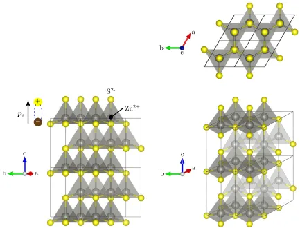
Figure 1.5: Crystal unit cell of PZT. (a) Above the Curie temperatureTC, the unit cell is cubic and non-ferroelectric. (b) Below the Curie temperature, the unit cell is tetragonal and ferroelectric.

switching occurs before electric breakdown. Common examples are lead zirconate titanate (PZT), which is widely used in industry and will be examined in experiments later, and barium titanate (BaTiO3). Many other types of ferroelectric materials exist (see e.g. (Fatuzzo and Merz,1967;Jona,

(30)

1.1.3

Microstructure: Domains and domain walls

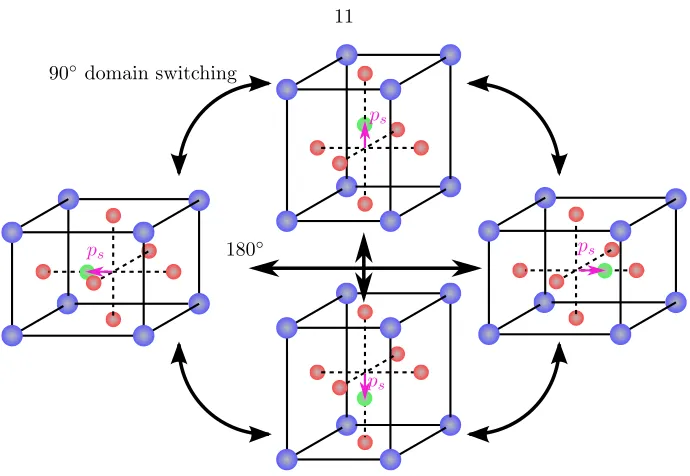
The spontaneous polarization in ferroelectrics gives rise to a complex microstructure. This is due to the different possible directions of the spontaneous polarization. For example, considering Fig.1.5, if PZT forms a single-crystal at high temperature (i.e. in the cubic phase) during manufacturing (e.g. via sintering) but is then allowed to cool to room temperature, the crystal transforms to the tetragonal (ferroelectric) phase. Although Fig. 1.5 shows the spontaneous polarization pointing upwards, there is a total of six equivalent directions, as shown in Fig. 1.6. Switching between two states results in either so-called 90◦ or 180◦ domain switching depending on the rotation angle the polarization vector undergoes. Along with the changing polarization is a spontaneous strain associated with 90◦ domain switching due to the elongation of the unit cell. Materials tend to minimize the self-generated electric field (i.e. avoid having the entire crystal with the same orientation) as well as minimize the elastic energy (i.e. avoid 90◦ domain walls due to the strain mismatch). These two competing effects produce microstructure in sufficiently-large single-crystal ferroelectrics. Regions in the crystal with the same polarization orientation are called domains

and the interfaces between those regions are called domain walls. If the relative orientation of polarization between two domains is 90◦, the interface is referred to as a 90◦domain wall. Similarly, 180◦ domain walls separate domains where there relative orientation of polarization is 180◦.

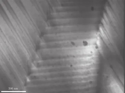
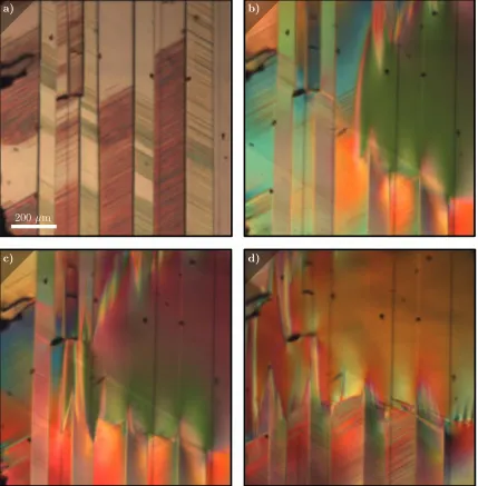
The microstructure in ferroelectrics can be visualized using various approaches. On the largest scale (e.g. millimeters), optical methods such as polarized light microscopy (PLM) are commonly used. By passing polarized light through a ferroelectric single crystal, different domains with anisotropic indices of refraction alter the polarized light, which is recorded in a camera (different colors correspond to different domain orientations). The approach is limited to thin single-crystal specimens that are transparent (polycrystals would cause significant scattering). An example image of ferroelectric domains in single-crystal lead magnesium niobate-lead titanate (PMN-PT), which is a type of ferroelectric, is shown in Figs.1.7(a) and (b). It can be seen that the microstructure tends to form a hierarchical lamination structure. Zooming in closer using piezo-force response microscopy (PFM), finer-scale domain laminates can be seen in Figs. 1.7(c) and (d). PFM is a type of scanning probe microscopy method similar to atomic force microscopy (AFM) where the cantilever tip is charged and thus experiences forces due to the electric polarization of the material. Typically, PFM is used to take images on the nano- to micron-scale. On the nanoscale, Fig.1.8

(31)

ps

ps 180◦

ps ps

[image:31.612.134.479.73.311.2]

90◦domain switching

Figure 1.6: There are six equivalent directions of the spontaneous polarization in PZT: the four shown here as well as in and out of the page.

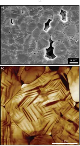
Manufacturing large single-crystal ferroelectrics is difficult and expensive. The largest sizes that are typically available have side lengths on the order of millimeters. Therefore, most structural applications of ferroelectrics utilize their polycrystalline form (i.e. ferroelectric ceramics). Ferro-electric ceramics are commonly manufactured using powder compaction and sintering processes. Thus, the original grain size of the powder governs the resulting grain size in the material. How-ever, in addition to grains, the microstructure of ferroelectric ceramics still contains domains within individual grains. This can be seen in Fig.1.9. One can see the granular structure formed through powder compaction and sintering in Fig.1.9(a) using Scanning Electron Microscopy (SEM), while zooming in closer using AFM, one can see the domain lamination structure within individual grains in Fig.1.9(b).

(32)

appli-200µm 50µm

4µm 4 µm

a) b)

[image:32.612.93.523.136.561.2]

c) d)

(33)

[image:33.612.96.521.194.512.2]

200 nm

(34)

Figure3. AFMimagesofanindividualgrainafter(a)rstpolishingandrstetching,(b)repolishingand(c)secondetching.

(a)(b)

Figure4. AFMimagesofanindividualgrain(a)beforedepolingand(b)afterdepoling. a)

5 µm

b)

[image:34.612.177.436.80.554.2]

1µm

(35)

cation of an electric field as shown in Fig. 1.10. By applying an electric field, domains change orientation to align with the field, resulting in a larger domain that grows as the field is increased. Similar behavior is observed when applying mechanical stresses where domains realign to reduce elastic energy. The evolution of domain structure affects the macroscopic mechanical response. For example, the PZT unit cell exhibits anisotropic elastic constants, therefore, different volume fractions of differently-oriented domains change the effective elastic constants of the material. In addition, the domain switching process takes time and dissipates energy, which leads to a time-dependent mechanical response, which is of interest in this study.

1.1.4

Applications

Over the years, piezoelectrics and ferroelectrics have become widely used in many applications. The most common materials are the various forms of PZT and lead-free BaTiO3, both of which are

ceramic materials. Piezoelectricity and ferroelectricity can exist in non-ceramics such as polymers (e.g. piezoelectricity and ferroelectricity in polymers were first discovered by Japanese scientists in polyvinylidene fluoride (PVDF) (Kawai,1969; Tamura et al.,1974)). The use of such polymer materials is attractive for light-weight applications in aerospace (Carvell and Cheng,2010;Wegener,

2008) and in foams (Frioui et al.,2010;Iyer et al.,2014;Venkatesh and Challagulla,2013). However, their extremely high coercive field (as high as 50 MV/m) makes them an undesirable material for exploring and potentially tapping their behavior during domain switching. Therefore, ferroelectric ceramics with lower coercive fields will be investigated.

(36)

a) b)

c) d)

[image:36.612.93.522.118.555.2]

200 µm

(37)

1.2

Concepts of linear viscoelasticity

Although the theory of viscoelasticity is often discussed in the context of polymers, it is nonetheless applicable to ferroelectric ceramics. As a fundamental property of a viscoelastic material, the mechanical response depends on the loading history and loading rate (the reader is referred to the texts on viscoelasticity byLakes(1998) andChristensen(2003) for more details). Such a description applies to ferroelectrics; the evolution of the material’s domain structure requires that the loading history of the material (electrical and mechanical) be known in order to predict how it will respond at a given point in time. With this in mind, the constitutive equation for a viscoelastic material is commonly postulated to be of the form

σ(t) =

Z t

−∞

C(t−t0)dε(t

0₎ dt0 dt

0_, _(1.3)

where σ is the Cauchy stress tensor, C is the time-dependent modulus tensor, ε is the linearized strain tensor, and t is time. For current purposes, materials are assumed isotropic with time-dependent Young and shear moduli,E(t) and G(t), respectively. For the cases of uniaxial tension and simple shear, the relevant constitutive equations relate the longitudinal strainεand shear strain

γto the longitudinal stressσand shear stressτ, respectively, as

σ(t) =

Z t

−∞

E(t−t0)dε(t

0₎ dt0 dt

0_, _τ₍_t_{) =}Z

t

−∞

G(t−t0)dγ(t

0₎ dt0 dt

0_. _(1.4)

For the experiments performed in this work, harmonic motion is assumed and initial transient effects are assumed to be damped out quickly. Therefore, (1.4) can rewritten by assuming harmonic forms for the stresses and strains:

ε(t) = ˆεeiωt, σ(t) = ˆσeiωt, γ(t) = ˆγeiωt, τ(t) = ˆτ eiωt, (1.5)

(38)

yields

σ(t) =

−ω

Z t

−∞

E(t−t0) sinωt0dt0+iω

Z t

−∞

E(t−t0) cosωt0dt0

ε(t),

τ(t) =

−ω

Z t

−∞

G(t−t0) sinωt0dt0+iω

Z t

−∞

G(t−t0) cosωt0dt0

γ(t),

(1.6)

where Euler’s formula,eiωt _{= cos}_ωt₊_i_sin_ωt _{has been used. By inspection of (}_1.6_{), one can see} that the terms in brackets are the apparent complex-valued Young and shear moduliE∗ and G∗, respectively, i.e.

σ(t) =E∗ε(t), τ(t) =G∗γ(t). (1.7)

In general, a complex number can be fully described by its magnitude and argument (i.e. z=Reiθ_). Therefore, the measurements of the dynamic moduli, |E∗| and|G∗|, and phase angles, δE and δG describe the complex Young and shear moduli, respectively. Mathematically, these quantities are,

|E∗|=p[Re(E∗_)]2_{+ [Im(}_E∗_)]2₌|ˆσ|

|ˆε|, tanδE=

Im(E∗)

Re(E∗₎ = tan(argε−argσ),

|G∗|=p[Re(G∗_)]2_{+ [Im(}_G∗_)]2₌ |ˆτ|

|ˆγ|, tanδG=

Im(G∗)

Re(G∗₎ = tan(argγ−argτ),

(1.8)

(39)

σ(t)

ε(t)

σ(t)

ε(t)

ˆ

σ

ˆ

ε

δ

t 1.5

0.1 0.05 tanδ= 0

σ

ε

Figure 1.11: An example experiment to measure the viscoelastic properties of a material (i.e. the dynamic Young modulus and loss tangent) using harmonic loading in a DMA setup (an image of a Bose Electroforce is shown here).

1.3

Motivation

With the basic concepts of ferroelectricity and viscoelasticity reviewed, the motivation for study-ing the dynamic response of ferroelectrics is presented. The study of ferroelectric ceramics as energy absorbing materials (in particular for reducing vibrations in structures) has been ongoing for the past several decades. To this point, such applications can be separated into two categories, where the material is either passively or actively controlled in order to mitigate vibrations. Within these two categories are more specific methods to absorb energy. A typical method for creating passively-controlled energy absorbers is to short-circuit the ferroelectric material through a shunt resistor (Bachmann et al., 2012; Cross and Fleeter, 2002;Guyomar et al., 2008;Hagood and von Flotow,1991); a strain-induced voltage on the surface of the ferroelectric specimen creates a cur-rent that dissipates energy through the resistor via heating. Similarly, others have investigated embedding ferroelectric inclusions in a conducting metal matrix, where current generated by a strain-induced voltage in the inclusion is dissipated in the metal matrix via Joule heating (Asare et al.,2012; Asare, 2004, 2007;Goff, 2003; Goff et al., 2004; Kampe et al., 2006; Poquette,2005;

Poquette et al., 2011). This type of material is difficult to manufacture due to depolarization of inclusions at high temperature. An alternative is to actively control the ferroelectric material via controlling an applied voltage to cancel out vibrations (Arafa and Baz,2000;Bailey and Hubbard,

(40)

Table 1.1: Structural damping approaches and some of the typical loss tangents achieved.

passive loss tangent

high-damping material layers in plates and beams >1 (Capps and Beumel,1990;Wetton,1979)

tuned mass damper (Taranath,1988) –

piezoelectric damping via shunt resistor (Bachmann et al.,2012) 0.001−1.0 piezoelectric-metal matrix composites (Asare et al.,2012) 0.01

active loss tangent

vibration canceling –

piezoelectrics during temperature-induced phase changes (Cheng et al.,1996) <0.02 stress induced domain switching (Chaplya and Carman,2002a) <0.1

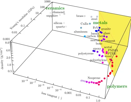
Ermanni, 2004; Liu et al., 2010; Ngo et al., 2004; Richard et al., 1999; Tremaine, 2012; Trindade and Benjeddou,2002). Additionally, the viscoelasticity of ferroelectrics has been studied but only under small electric fields (Budimir et al., 2004; Burianova et al., 2008) (i.e. when there is no microstructure evolution due to domain switching). As described in Section1.2, a common metric for evaluating the ability of a material to absorb vibrational energy is to measure its loss tangent, tanδ. The higher the loss tangent, the more the material reduces vibrations. The problem with the passive methods is that they produce relatively small loss tangents (typically tanδ < 0.01) over most mechanical frequencies while only achieving significant damping near the resonance of the system (typically tanδ= 1.0). Furthermore, active methods add complexity and are limited by the strains and forces achievable by piezoelectricity, which makes their application in stiff, mas-sive structures challenging. A summary of the mechanical damping reached by the aforementioned methods as well as others is shown in Tab.1.1.

(41)

10−8

10−7 10−6

10−5

0.001 0.01

0.1 1.0 10−4

loss_tangen t (–) densit y (g/c m 3)

0.5 1.0 2.0 4.0 8.0

Young’s mo

dulus (GP

a)

0.001 0.01

[image:41.612.97.517.179.506.2]

0.1 1 10 100 1000 diamond sapphire silicon quartz

ceramics

metals

polymers

brass steel CuZn aluminum FeV basalt carbon fiber granite glass cement mortar bone polystyrene epoxy acetal PMMA PTFE wood polyethylene Neoprene

(42)

switching) is studied. In particular we examine the viscoelastic response and compare with other methods for vibration control. This approach was first examined about a decade ago but little has been studied since then. In particular,Chaplya and Carman(2001a,b,2002a,b) examined the dis-sipation in ferroelectrics due to stress-induced domain switching whileJim´enez and Vicente(1998,

2000) investigated dissipation from electric field-induced domain switching.

Exploring the viscoelastic properties of electromechanically-coupled materials such as ferro-electrics may lead to new avenues of creating materials with controllable viscoelasticity. In a similar manner to metallic materials, for which damping is the macroscopic manifestation of the motion of point defects (Snoek,1941;Zener,1948) or dislocations (Eshelby,1949;Granato and L¨ucke,2004), of grain boundary activities (Kˆe, 1947), or of heterogeneous thermoelastic mechanisms (Bishop and Kinra, 1995; Zener, 1937, 1938), additional damping can arise from domain wall motion in materials such as ferromagnets (Burdett and Layng,1968; Gilbert,2004;Wuttig et al.,1998) and ferroelectrics (Abrahams et al.,1968;Harrison and Redfern,2002). The motion and interaction of domain walls in ferroelectrics with defects (Kontsos and Landis, 2009; Schrade et al., 2007) pro-duce Debye peaks of dielectric losses (Gentner et al., 1978; Xu et al., 2001; Zhou et al., 2001) as well as increased mechanical damping (Arlt and Dederichs,1980;Asare et al.,2012) and hysteresis effects (Cao and Evans,1993;Chen and Viehland,2000; Schmidt,1981). This effect becomes even more pronounced when the material is subjected to an electric field above the coercive field (Merz,

1954;Miller and Savage,1958,1960;Tatara and Kohno,2004;Yin and Cao,2001). Thus, by care-fully controlling an applied electric field, microstructure kinetics via domain wall motion and the resulting time-dependent response of ferroelectrics can be controlled. Therefore, the goal of the thesis research was to fully characterize the kinetics of domain switching in ferroelectrics (through experiments and modeling) for creating high stiffness, high damping structural materials and for new methods of actuation.

1.4

Outline

(43)

changes, due to domain switching, are investigated. Furthermore, the influence of domain switching on the overall structural response of ferroelectric specimens (i.e. throughout the resonance spec-trum) is determined, which is important for understanding their impact in structural applications. A continuum-mechanics model is also developed to capture experimental measurements and predict the behavior of new materials to optimize their viscoelastic response. With a better understand-ing of the viscoelastic properties of ferroelectrics, proof-of-concept experiments are performed to demonstrate potential applications of domain switching in set-and-hold actuators and for structural damping.

(44)

Chapter 2

Broadband Electromechanical

Spectroscopy

The following sections follow from our previously published papers 1 ₍_{le Graverend et al.}_, ₂₀₁₅_;

Wojnar et al., 2014), however some additional details are provided. Understanding and ultimately technologically exploiting the electro-thermo-mechanically-coupled time-dependent properties of materials (e.g., of ferroelectric materials or of composites containing ferroelectric phases) requires currently-unavailable measurement capabilities. Indeed, most available experimental methods for characterizing viscoelastic materials are commonly performed by forced and free vibration test-ing (Zhou et al.,2005b) and are applicable over rather restricted portions of the time and frequency domains (Ferry,1980).

Dynamic Mechanical Analysis (DMA) (Lakes,2004), for instance, mechanically deforms samples by time-harmonic bending, torsion, or tension/compression. DMA apparatuses are versatile and experiments can be performed over wide ranges of ambient conditions; temperatures ranging from -150 to 600◦C can be achieved in certain DMA setups (TA Instruments, 2015). However, the frequency range of DMA depends significantly on the sample and on the test apparatus used. For example, state-of-the-art DMA devices (Perkin Elmer,2014) typically cover at most 0.001 to 600 Hz, and their use is also limited to a maximum specimen stiffness of less than 1 GPa, which 1_{The method and experimental setup was described in le Graverend, J.B., Wojnar, C., Kochmann, D., 2015.}

(45)

excludes testing of ceramics and metals in general. Usually, the inertia of the grips in contact with specimens in DMA limits the maximum driving frequency of the apparatus. Also, gripping or otherwise contacting stiff, brittle materials such as ferroelectrics (and ceramics) without damaging the specimen is difficult in practice, hence a contactless measurement approach is needed.

The Inverted Torsion Pendulum (ITP) is such a method that uses contactless techniques (Kˆe,

1947). However, the ITP is typically used for low-frequency experiments (10−5 to 10 Hz), which may be too slow for observing the influence of microstructural processes in ferroelectrics such as domain wall motion (Jim´enez and Vicente,2000;Miller and Savage,1958). Like DMA, the ITP is also versatile and experiments have been performed over wide ranges of temperatures from cryogenic to elevated temperatures (-285◦C to 1500◦C) under vacuum (D’Anna and Benoit, 1990; Gadaud et al., 1990; Gribb and Cooper, 1998; Woirgard et al., 1977). The ITP has mainly been used for characterizing metals and ceramics with Young moduli ranging from 10s to 100s of GPa. Its contactless approach of applying forces electromagnetically to specimens makes the ITP attractive for testing ceramics.

Although primarily used for measuring elastic moduli (Migliori et al., 1993), Resonant Ultra-sound Spectroscopy (RUS) can determine the frequency-dependent viscoelastic moduli by scanning the specimen’s resonance spectrum in a double-transducer actuator-sensor setup (Lee et al.,2000). The frequency range of RUS instruments is larger than DMA as it does not require a mechanical driver but relies upon piezoelectric actuation. However, it is affected by the piezo-cells’ resonance frequencies and practical limitations. For typical specimen sizes, (Lee et al.,2000) and (Zadler et al.,

2004) (for example) report RUS results from about 10 kHz to 10 MHz and from 5 kHz to 100 kHz, respectively. RUS has been performed under various ambient conditions such as temperatures rang-ing from -193 to 247◦C (Kuokkala and Schwarz,1992) and elevated pressures (Zhang et al.,1998), but not under vacuum, which is desirable for reducing spurious damping. In addition, the specific specimen geometry required by RUS makes applying uniform electric fields via surface electrodes difficult. Thus, electromechanical loading in RUS has not been attempted. A similar method called the Piezoelectric Ultrasonic Composite Oscillator Technique (PUCOT) (Daniels and Finlayson,

2006) tracks the specimen’s resonance spectrum in a forced-vibration cantilever configuration. In a similar fashion to DMA, Broadband Viscoelastic Spectroscopy (BVS) performs bending and torsion but uses contactless techniques (Dong et al.,2008; Lakes and Quackenbusch, 1996;Lakes,

(46)

laser-Table 2.1: Comparison of the various viscoelastic characterization methods with BES. BES is the only method that allows for a wide range of viscoelastic materials to be tested in a contactless fashion and in a vacuum environment while simultaneously controlling the temperature and applying electric fields.

method bandwidth moduli temp. e-field vac. contactless

DMA 10-3 _{to 10}2 _Hz _{up to 1 GPa} _{-150 to 600}◦_C _– _– _–

RUS 104 _{to 10}7 _Hz _tan_{δ <}₁₀-2 _{-193 to 247}◦_C _– _– _–

ITP 10-5 _{to 10 Hz} _{10 to 10}3_GPa _{-268 to 1400}◦_C _–

X X

BVS 10-6 _{to 10}5 _{up to 10}4 _GPa _{up to 160}◦_C _– _–

X BES 10 to 104 _Hz _{up to 10}4 _GPa _{up to 400}◦_C

X X X

detector setup. Thus, BVS offers higher sensitivity and finer resolution than DMA and is capable of scanning many decades of frequency (Brodt et al.,1995) with considerably lower compliance and less spurious damping. Moreover, the contactless testing prevents damaging of the specimens. BVS data has been reported for the range of roughly 10−6 to 105 Hz, i.e. covering approximately 11 decades of time and frequency (Lee et al.,2000). Of course, the exact frequency range depends on the test instrument, the electronic function generator, the laser detector used, and on the sample. Temperatures of up to 160◦C have been reached in the BVS apparatus used in (Dong et al.,2011,

2008,2010) using convection heating via air flow, which unfortunately can lead to spurious damping. The capabilities of the aforementioned methods are summarized in Tab. 2.1. Despite all these techniques,electric fields and mechanical loads over significant ranges of frequency have not been in-dependently applied before, which is necessary for fully-characterizing the thermo-electromechanical response of ferroelectrics. Thus, a different method and setup is needed.

(47)

test a wide range of viscoelastic materials under combined temperature and electric field control in a vacuum environment, while still having the capability to apply a wide range of mechanical frequencies as in BVS. A wide frequency range is important for characterizing the kinetics of domain switching as well as understanding its impact on structural resonance. We note that the BES method is more general than the specific apparatus presented here. In Chapter3, using BES, the dynamic stiffness and damping in bending and torsion of a ferroelectric ceramic, viz. PZT, are measured during electric field-induced domain switching. Moreover, experiments performed in air and under vacuum are compared to quantify the influence of the surrounding air on the measured dynamic stiffness and damping.

2.1

Materials and methods used in Broadband

Electrome-chanical Spectroscopy

To study a wide range of materials with thermo-electromechanically coupled properties from soft polymers such as PVDF (with a typical Young modulus of 3 GPa (Tamura et al., 1974)) to stiff ferroelectric ceramics (which are studied here and have Young moduli on the order of 100 GPa) and composites containing ferroelectrics (whose dynamic moduli can be as high as 104 _{GPa (}_Jaglinski

et al., 2007)), the specimens are tested in bending and/or torsion, as opposed to uniaxial tests. Specimens with cantilevered beam geometry are gripped on one end and a bending and/or torsional moment is applied to their free end, as shown in a schematic of the apparatus in Fig. 2.1. The cantilever beam setup is best suited for testing materials under time-varying temperatures and electric fields as both of which may cause eigenstrain in the material. The minimal grip contact with cantilever beams (compared to 3-point or 4-point bending setups) minimizes the amount of internal stresses arising from eigenstrain, which may influence the material response. In a similar manner to BVS (Lakes, 2004), bending and torsional moments are applied through Helmholtz coils via a permanent magnet attached to the specimen’s free end. Specimen deflection/twist is captured via a laser-detector set-up as shown in 2.2(a). Adding to the capabilities of BVS, an electric field is applied using surface electrodes on the specimen and electric displacements are measured via a Sawyer-Tower circuit connected to the grips (Sawyer and Tower, 1930; Sinha,

(48)

vertical coils used for bending horizontal coils used for torsion

permanent magnet

grip electrode vacuum

mirror

specimen electrodes

grips

position sensor laser

lock-in amplifier

waveform generator in ref.

waveform generator high-voltage amplifier

scope

V(t) = ˆV cosωt u(t) = ˆucos(ωt+δ)

t _{t H}y

Hz

Hy

Hz

My

Mz

µ

ex, dx ˆ

u,tanδ

[image:48.612.93.517.77.347.2]

chamber window

Figure 2.1: Schematic of the apparatus showing the specimen gripped in the center. Above the specimen are the two pairs of Helmholtz coils used for bending and torsion tests as in BVS. The coils are shown in their raised position allowing for the specimen to be positioned. Once the specimen is gripped in place, the coils are lowered over the specimen such that the magnet is located at the intersection of the two coil axes. The specimen and coils are placed inside a vacuum chamber with a window for the laser beam to enter and reflect back to the position sensor outside. In the top-left corner appears the lock-in amplifier set-up connected to the position sensor with the applied voltage to the coils used as the reference signal. The bottom-right corner shows the Sawyer-Tower circuit used.

(49)

HeNe laser

BES (in operation)

BES (chamber open)

test device

specimen grip turbomolecular vacuum pump

water cooling supply

double-wall vacuum chamber (with stainless steel/Kodial window)

position sensor

clamp for magnet/ mirror attachment torsional coils

bending coils permanent

magnet and mirror