Application of generalized intervention analysis model

© 2019 Scholars Journal of Economics, Business and Management | Published by SAS Publishers, India 17 ISSN 2348-8875 (Print) | ISSN 2348-5302 (Online)

Journal homepage:http://saspjournals.com/sjebm

Application of Generalized Intervention Analysis Model

Xiaohua HU1*, Zhongwei Zhang2

1_{School of mathematics and statistics, Hainan Normal University}

2_{School of Agricultural, Computational and Environmental Sciences, Faculty of Health, Engineering and Science, University of Southern Queensland,} Australia

*Corresponding author: Xiaohua HU | Received: 12.01.2019 | Accepted: 13.01.2019 | Published: 30.01.2019

DOI:

10.21276/sjebm.2019.6.1.4

Abstract

Original Research Article

In this paper, the intervention analysis model has been generalized in the sense that its intervention function either being a jumping function used to describe the continuing intervention or a unit impulse function used to describe the transient intervention has been replaced with a unified function,



exp(

-



(

t

-

T

))

, which represents an intervention process,



denotes the amplitude (or strength) of the impact of intervention events at intervention time,



denotes the decay factor of continuing process. Applying the generalized model to predict the Gross Domestic Product (GDP) of Hainan province from 1989 to 2016, as a Government intervention was introduced in 2010, results in a 60% of improvement in terms of the Root Mean Square Error (RMSE), when compared with the original model.

Keywords: intervention event, jump function, unit impulsive function, generalized intervention analysis model, Hainan GDP.

JEL Classification: C53.

Copyright @ 2019: This is an open-access article distributed under the terms of the Creative Commons Attribution license which permits unrestricted use, distribution, and reproduction in any medium for non-commercial use (NonCommercial, or CC-BY-NC) provided the original author and source are credited.

INTRODUCTION

The invention analysis model was initially proposed in 1975 by Statistics Prof. Box and Tiao of the University of Wisconsin, US, in a journal paper (Box [1]), which was primarily applied to quantitatively analyze and discuss the effects on economics, which caused by the sudden changes of economic policies or occurring events. Enforcement of economic polices and intervention of sudden events occurring, such as political events, natural disasters and economic policies all called interventions, must have some influences on economic developments, even ultimately restructure the economics (Feng [2]).

An intervention variable is the main variable in the intervention analysis model, there are two types of intervention variables: one is continuous variable and another is transient variable. The continuous variable is keeping on influence after the moment of its occurring. A continuous variable is described by a jumping function, as follows:

) 1 ( event

on interventi after the

, 1

event on interventi the

before , 0   

  

） （

） （

T t

T t S_tT

While the transient variable has some effect at the moment of its occurring, for which a unit impulsive function can be used to represent,

)

2

(

event

on

interventi

after the

,

0

event

on

interventi

the

before

,

1













）

（

）

（

T

t

T

t

P

T

t

Here, we would introduce a time related intervention function as represented

) 3 ( ) ( event on interventi after

and of at time ,

) ( event on interventi prior to

, 0

) (

  

 

 _{ }

T t e

T t HtT



_tT

where



and



are constants, and called the amplitude (or strength) of the intervention event, the decay factor, respectively, at the

T

moment.

It is apparent that

H

_tTin (3) is more reasonable in describing the intervention while a sudden event occurred.

That is to say



is the amplitude (or strength) of intervention at the time

T

;



is the speed of intervention decaying.

1, if



in (3) is large, and





1

, then the intervention decay fast, and intervention duration is short, then (3) should approach to (2).

2, if



in (3) is small, and





1

, the the intervention last long, (3) should be closer to (1).

In other words,

S

_tT in (1) and

P

_tT in (2) are special cases of

H

_tT in (3). In fact, the intervention variables in

(1) and (2) only describe two extreme cases, namely, long-term intervention of the same intensity and instantaneous intervention. In a general way, the intervention of unexpected events is often a dynamic process, there is strong or weak for the intervention, there is short and long for the process. Obviously, (1) and (2) are two extreme cases of (3), and idealized. Consequently, (3) has generalized (1) and (2), to be more practicable in real. The intervention analysis model of continuous variable is

)

4

(

...

1

_{1 2}

T t r r b

t

S

B

B

B

B

X



















The intervention analysis model of transient variable is

)

5

(

...

1

1 2

T t r r

t

P

B

B

B

X



















The generalized intervention model is

)

6

(

...

1

_{1 2}

T t r r b

t

H

B

B

B

B

Z



















where



,

b

,

r

,



i

,

i



1

,...,

r

,

are the parameters to be estimated,

B

is the lag operator.

As the youngest province and the biggest economic special zone in China after 1989, Hainan province has achieved tremendously progress, in terms of its GDP figure, since 1989 to 2009, with her special geographic location and pleasant climate conditions. On Jan 4, 2010, the State Council of China issued a Governmental document, which aims to turn Hainan island (or Hainan province ) into a world tourist attraction. This policy, considered as a sudden intervention event, has significantly changed the economic development of Hainan province, in particular the GDP figures. Since then, Hainan has come into a completely new era of economic development. In this study, we are interested in the amplitude of intervention and focus on the continuing influences of the intervention.

© 2019 Scholars Journal of Economics, Business and Management | Published by SAS Publishers, India 19

M

ODELING AND EMPIRICAL ANALYSIS

Here GDP is denoted by

GDP

_t, and

t

is another time variable, representing the calender year,

t



1

,

2

,...,

28

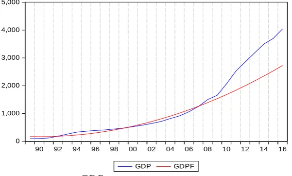
, which represents the year 1989, 1990, ..., 2016.

GDP

_t time plot is shown in Figure 1, sample data from Hainan Bureau

of Statistics (www.stats.hainan.gov.cn) is shown in Table 1. Due to the sudden event occurred at year 2010, it's

noticeable there was an accelerated increasing rates in

GDP

_t data, which was clearly higher than the previous

increasing rates since that year.

0 1,000 2,000 3,000 4,000 5,000

90 92 94 96 98 00 02 04 06 08 10 12 14 16

GDP GDPF

Fig-1:

GDP

_t and its trend extrapolation plot

Table-1: Hainan Province GDP data from 1989 to 2016 (in 100 million Chinese yuan) year 1989 1990 1991 1992 1993 1994 1995 1996 1997 1998 GDP 91.32 102.42 120.52 184.92 260.41 331.98 363.25 389.68 411.16 442.13

year 1999 2000 2001 2002 2003 2004 2005 2006 2007 2008 GDP 476.67 526.68 579.17 642.73 713.96 819.66 918.75 1065.67 1254.17 1503.06

year 2009 2010 2011 2012 2013 2014 2015 2016 GDP 1654.21 2064.5 2522.66 2855.54 3177.56 3500.72 3702.76 4044.51

Effect sequence and Regression model of Intervention

The

GDP

_t data of Hainan province prior to 2009 can be regressed by a quadratic function,

t



1

,...,

21

)

7

(

8

.

3

55

.

15

53

.

183

t

t

2

GDP

_t







where the fitting goodness:

R

2= 0.97. Use (7) to extrapolate the

GDP

_t data after year 2010,

t



22

,...,

28

, see Figure

1. these data can be regarded as the actual

GDP

_t without the intervention.

Let

Z

_tbe the effect sequences that are the differences between the extrapolated

GDP

_t data and the actual

t

[image:3.595.148.449.178.359.2]

GDP

data after year 2010. Table 2 is the effect sequence of intervention after year 2010.

Table-2: Effect sequences of Intervention after 2010

t

22 23 24 25 26 27 28

t

Z

382.6736 685.2776 854.997 1006.252 1151.042 1167.108 1315.28

Here by the use of the original model (4) and EViews 8.0, on

Z

_t in Table 2, we can get the estimate parameters as: [image:3.595.119.473.643.684.2]

)

8

(

744

.

0

1

214

.

379

ˆ

1

ˆ

_T t T t t

S

B

S

B

Z













When

T



20

,(or 2010 year)

379

.

214

,

ˆ

₀

.

744

ˆ









,

R

2



0

.

956

,

RSE



11513

.

87

Again, by the use of the generalized intervention model (6), these parameters become

t t

t

Z

e

Z

( 0.082)

1

79

.

513

425

.

0

_







)

9

(

425

.

0

1

513

.

79

ˆ

1

1

T 0.082t

t t

e

B

H

B

Z











When

T



20

425

.

0

ˆ

,

513

.

79

ˆ

,

082

.

0

ˆ















_,

R

2



0

.

975

,

RSE



6358

.

149

Obviously, the

RSE

(6358.149) of (9) is smaller than that (11513.87) in (8), the

R

2(0.975) of (9) is bigger than that (0.956) in (8).

When

T



2000

year,



ˆ



79

.

513

, and



ˆ





0

.

082

,

it indicates that (3) is better than (1), when it comes to describe the intervention.

Purified Sequence and Fitting Model

We calculate the purified sequence. The purified sequence is a sequence that it is eliminated the effects of

intervention, or it is the difference between the actual

GDP

_t and the intervened effect value

Z

_t.

By the use of (8), we get

)

10

(

28

,...,

2

,

1

,

22

,

744

.

0

1

214

.

379

ˆ

1

ˆ

















S

T

t

B

GDP

S

B

GDP

y

_{t t t}T _{t t}T





Similarly, by the use of (9), it becomes

)

11

(

28

,...,

2

,

1

,

22

,

425

.

0

1

513

.

79

ˆ

1

1

0.082

















e

T

t

B

GDP

H

B

GDP

x

_{t t t}T _t t



Prior to Jan, 2010, there was no intervention, the first 21

GDP

_t data (1654.21) in Table 1 should be the net

data. The

GDP

_t figure of year 2010, however, was recorded at the end of year, so the

GDP

_t data at that year was

effected by the intervention. The purified

GDP

_tfigure should be simplified as the average value of the

GDP

_t data of

year 2009 and 2010. or 1859.3. The purified sequence after 2010 is shown in Table 3.

By the use of (4), (8) and (10), the fitting model,

y

_t, is

)

12

(

738

.

3

357

.

13

557

.

173

ˆ

2

t

t

y

_t







where

R

2



0

.

9915

,

RSE



151404

.

3

, By the use of (6), (9) and (11), the fitting model,

x

_t, is

)

13

(

784

.

3

303

.

14

744

.

176

ˆ

2

t

t

x

_t







[image:5.595.148.447.75.141.2]

© 2019 Scholars Journal of Economics, Business and Management | Published by SAS Publishers, India 21

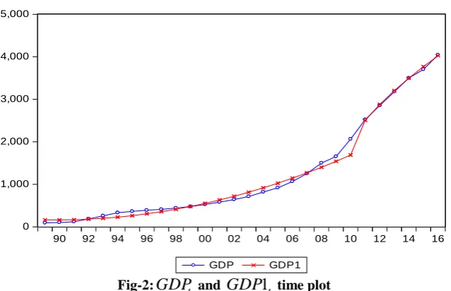
Table-3: The purified sequences after 2010( based on (1) and (3) )

t

22 23 24 25 26 27 28

t

y

1859.3 1858.6 1982.2 2148.5 2355.7 2471.5 2749.1

t

x

1859.3 1829.8 1985.1 2182.1 2398.2 2496.4 2730.6

Intervention Analysis Modeling

By use of (4), (8), (10) and (12), we can obtain an intervention analysis model,

GDP

1

_t,is

T t t t

S

B

y

GDP





ˆ

1

ˆ

ˆ

1







)

14

(

744

.

0

1

214

.

379

738

.

3

357

.

13

557

.

173

1

_t 2

S

_tT

B

t

t

GDP











Where

)

15

(

)

22

(

2010

at year

and

after

,

1

)

22

(

2010

prior to

,

0













t

t

S

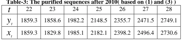
_tT

After the use of (14) and (15), the predicted

GDP

_t are shown in Table 4.

The Root Mean Squared Error (

RMSE

) between the Actual

GDP

_tand the predicated data

GDP

1

_t is 96.96, [image:5.595.62.470.547.763.2]

denoted by

RMSE

₁.

GDP

_t And

GDP

1

_t time plot as Figure 2.

Table-4: Predicated Data by use of (14) and (15)

year 1989 1990 1991 1992 1993 1994 1995 1996 1997 1998

t

GDP1 163.9 161.7 167.1 179.9 200.2 228.0 263.2 305.9 356.1 413.8

year 1999 2000 2001 2002 2003 2004 2005 2006 2007 2008

t

GDP1 479.0 551.6 631.7 719.3 814.4 916.9 1026.9 1144.5 1269.4 1401.9

year 2009 2010 2011 2012 2013 2014 2015 2016

t

GDP1 1541.8 1689.2 2508.1 2879.8 3205.4 3498.61 3769.7 4026.1

On the other hand, if we use (6), (9), (11) and (13), then the intervention analysis model,

GDP

2

_t,is

T t t t

H

B

x

GDP



ˆ

1

1

ˆ

2







)

16

(

425

.

0

1

1

78

.

3

303

.

14

744

.

176

2

_t 2

H

_tT

B

t

t

GDP











Where

)

17

(

)

22

(ie.t

2010

at year

and

after

,

513

.

79

22)

<

(ie.t

2010

prior to

,

0

) 082 . 0 (











_{ t}

T t

0 1,000 2,000 3,000 4,000 5,000

90 92 94 96 98 00 02 04 06 08 10 12 14 16

GDP GDP1

Fig-2:

GDP

_t and

GDP

1

_t time plot [image:6.595.139.458.66.272.2]

After the use of (16) and (17), the predicted

GDP

_t are shown in Table 5.

Table-5: Predicated Data by use of (16) and (17)

year 1989 1990 1991 1992 1993 1994 1995 1996 1997 1998

t

GDP

2

166.2 163.2 167.8 180.0 199.8 227.1 262.0 304.5 354.5 412.1

year 1999 2000 2001 2002 2003 2004 2005 2006 2007 2008

t

GDP

2

477.3 550.0 630.3 718.2 813.6 916.6 1027.2 1145.4 1271.1 1404.4

year 2009 2010 2011 2012 2013 2014 2015 2016

t

GDP

2

1545.2 1693.6 2542.5 2883.6 3179.83 3465.5 3755.6 4057.0

0 1,000 2,000 3,000 4,000 5,000

90 92 94 96 98 00 02 04 06 08 10 12 14 16

GDP GDP2

Fig-3:

GDP

_t and

GDP

2

_t time plot

The

RMSE

between the Actual

GDP

_tand the predicated data

GDP

2

_t is 38.77, denoted by

RMSE

₂.

t

GDP

And

GDP

2

_t time plot as Figure 3. [image:6.595.125.471.317.655.2]

© 2019 Scholars Journal of Economics, Business and Management | Published by SAS Publishers, India 23

Improvement Percentage =

60

%

96

.

96

77

.

38

96

.

96

1 2

1









RMSE

RMSE

RMSE

C

ONCLUSION

In this paper, we have generalized the intervention analysis model from the theoretical aspect. The generalized model has been applied to fit the Hainan province GDP data from 1989 to 2016, compared with that of using the original model. We have established two models represented in (14),(15) and (16),(17). From the results (16) and (17) of generalized intervention analysis model (3) and (6), we can clear see there was a significant effect on Hainan GDP due to the introduction of Government intervention policy in 2010. Moreover, the amplitude of the intervention was

513

.

79





, and the decay factor is







0

.

082

. Improvement Percentage is 60%.

The generalized intervention analysis model has shown the superiority over the original model in terms of the

RMSE

values.

R

EFERENCES

1. Box GE, Tiao GC. Intervention analysis with applications to economic and environmental problems. Journal of the American Statistical association. 1975 Mar 1;70(349):70-9.

2. Feng Wenquan. Statistical Analysis Model of Policy intervention or Emergency impact. Statistics & Decision, 1990; 90,pp.8-9.

3. Gao Jingchuan. Study on the Effect of Investment Growth on the Economic Growth in Hainan. Statistics & Decision. 2012; 12, pp.334-337.

4. Zhang Qiang, Cui Qianqian, Ma Zhihui. Research on the Forecast for GDP of Xinjiang Based on the Intervention Analysis Model. J Chongqing Technol Business Univ(Nat Sci Ed). 2013; 13, pp.25-29.

5. Kong Zhaoli, Li Guohui, Shi Ming, Huang Meiting. Production on GDP of Hainan Province and Factors Analysis Based on GM (1, 1) and Principle Component Regression. Mathematics in Practice and Theory. 2016; 16,pp.66-80. 6. Guo Xiaoyuan. An empirical study on Industrial structure and Economic growth in Hainan Province. Spcial Zone

Economy. 2011; 11, pp.269-271.