Rochester Institute of Technology
RIT Scholar Works
Theses
Thesis/Dissertation Collections
3-31-2014
Analysis and Exploitation of Automatically
Generated Scene Structure from Aerial Imagery
David R. Nilosek
Follow this and additional works at:
http://scholarworks.rit.edu/theses
This Dissertation is brought to you for free and open access by the Thesis/Dissertation Collections at RIT Scholar Works. It has been accepted for inclusion in Theses by an authorized administrator of RIT Scholar Works. For more information, please [email protected].
Recommended Citation
Analysis and Exploitation of Automatically Generated Scene
Structure from Aerial Imagery
by
David R. Nilosek
B.S. Rochester Institute of Technology, 2008
A dissertation submitted in partial fulfillment of the
requirements for the degree of Doctor of Philosophy
in the Chester F. Carlson Center for Imaging Science
College of Science
Rochester Institute of Technology
March 31st, 2014
Signature of the Author
Accepted by
CHESTER F. CARLSON CENTER FOR IMAGING SCIENCE
COLLEGE OF SCIENCE
ROCHESTER INSTITUTE OF TECHNOLOGY
ROCHESTER, NEW YORK
CERTIFICATE OF APPROVAL
Ph.D. DEGREE DISSERTATION
The Ph.D. Degree Dissertation of David R. Nilosek has been examined and approved by the dissertation committee as satisfactory for the
dissertation required for the Ph.D. degree in Imaging Science
Dr. Carl Salvaggio, Dissertation Advisor
Dr. David Messinger
Dr. Nathan Cahill
Dr. Steven LaLonde
Analysis and Exploitation of Automatically Generated Scene
Structure from Aerial Imagery
by
David R. Nilosek
Submitted to the
Chester F. Carlson Center for Imaging Science in partial fulfillment of the requirements
for the Doctor of Philosophy Degree at the Rochester Institute of Technology
Abstract
iv
Acknowledgements
I joined the Digital Imaging and Remote Sensing Laboratory as a graduate student in the Winter of 2008. A numerous amount of people have helped me get to where I am today, and I would like to acknowledge and thank them all.
First and foremost, my thesis advisor Dr. Carl Salvaggio. Carl has officially been my advisor for about six years, but really he has been helping me along since before I completed my undergraduate degree. Beyond being an excellent academic mentor, I also consider him to be a good friend. He has helped me in both my professional and personal life, and I will be forever grateful for all he has done.
I would also like to thank my thesis committee: Dr. Dave Messinger, Dr. Nate Cahill, and Dr. Steve LaLonde. Dr. Messinger and Dr. Cahill were very helpful in shaping the direction of my dissertation work. They asked thought-provoking questions and made a number of very useful suggestions. I am grateful for their expertise and willingness to give advice. I am also very grateful for Dr. LaLonde’s being the external chair of my committee. We have a very limited academic relationship, however, I am astounded by the generosity and support he gave towards my dissertation process.
I would like to thank Dr. Derek Walvoord from ITT Exelis for advising me on a number of subjects throughout my work, and for always being able to answer any question I had. There have been a number of staff members in the DIRS Lab, whom have helped me along the way. I would like to thank Jason Faulring, for his unending technical support and expertise. I would also like to thank Scott Brown for his leadership, while I was working under the ESRI grant. I also would like to thank Mike Richardson, who helped me hone my presentation skills time and again. Thanks also goes to Bob Krzaczek for introducing me to git, asciidoc, and his numerous bits of coding advice.
Many thanks must be given to Cindy Schultz, without whom many DIRS graduate students, including myself, would be hopelessly lost. I would also like to thank Sue Chan for making sure I submitted everything on time (even when I was late). I’d also like to thank the many professors I had during my coursework, I am grateful to have attended an institution with such a wealth of knowledge and talent.
vi
me feel welcome in the office, and along with Sarah, helping turn my last name into a verb for computer malfunction. I would like to thank Shaohui and Mike for the many casual and technical conversations we had. They were helpful making office life enjoyable. I would also like to thank Katie, whom joined me in the quest for understanding C++ and Computer Vision. She helped me with my classwork as well as my research. I greatly appreciate all the help and friendship she’s given me over the years.
Many thanks also goes to Steve Schultz, from Pictometry Corp., whom not only gave me my first internship experience, but also hired me even before I had completed my dissertation. Thanks also to Amy Galbraith for being my mentor during my internship at Los Alamos National Laboratory.
I want to thank my friends and family. Mom, Dad, Andrea, and Courtney, thanks for all your support and always making me feel like I can accomplish anything. Uncle Ed and Lucy, thank you for supporting me through my undergraduate and graduate degrees, I would not have been able to do it without you. Curtis and Pat, you guys were some of the best roommates I could have asked for, thanks for helping me keep my life entertaining.
Contents
1 Introduction 1
1.1 Accurate Structure Extraction . . . 2
1.2 Physical Model Estimation . . . 3
1.3 Summary . . . 4
1.4 Contributions . . . 6
2 Background 7 2.1 Epipolar Geometry . . . 8
2.1.1 Projective Geometry . . . 8
2.1.2 Camera Model . . . 11
2.1.3 Stereo Geometry and the Fundamental Matrix . . . 15
2.1.4 Fundamental Matrix Derivation . . . 17
2.1.5 Relative Camera Pose Estimation . . . 20
2.2 Feature Detection, Description, and Matching . . . 24
2.2.1 SIFT . . . 25
2.2.2 Affine-SIFT . . . 28
2.2.3 DAISY . . . 29
2.2.4 Epipolar Line Matching . . . 31
2.2.5 Patch-Based Model . . . 33
2.3 Reconstruction Techniques . . . 35
2.3.1 Photogrammetric Approach . . . 35
2.3.2 Linear Triangulation . . . 37
CONTENTS ix
2.4.1 Feature Matching Optimization Using RANSAC . . . 39
2.4.2 Bundle Adjustment . . . 46
2.5 Deriving Geo-Accurate Structure Measurements . . . 55
2.5.1 Calculating Ts . . . 56
2.6 Discussion . . . 58
3 Methodology 60 3.1 Software . . . 61
3.2 Obtaining an Accurate Coordinate System . . . 64
3.2.1 Using Camera Position Estimates . . . 65
3.2.2 Using the Camera Model and Image Correspondence . . . 65
3.2.3 Using the Camera Model Directly . . . 67
3.3 Surface Reconstruction Methods . . . 68
3.3.1 Model Extraction Using RANSAC Plane Fitting and Alpha Shapes Boundary Extraction . . . 69
3.3.2 Voxel-Based Surface Estimation . . . 72
3.3.3 Constructing a Confidence Metric for Voxel-Based Estimated Sur-face Structure . . . 85
3.3.4 Using a Depth Map for Structure Segmentation . . . 88
3.4 Surface Attribution and Classification . . . 91
3.4.1 Reflectance Attribution Through Hyperspectral Imagery . . . 92
3.4.2 Surface Material Segmentation with R,G,B Spectral Information . . 97
3.5 Discussion . . . 103
4 Results and Analysis 105 4.1 Georegistration Analysis . . . 105
4.1.1 Georegistration Error Using DIRSIG Noiseless Sensor Model . . . . 107
4.1.2 Georegistration Error Using DIRSIG Noisy Sensor Model . . . 110
4.1.3 Reducing the SfM Error . . . 112
4.1.4 Using a Large Number of Images . . . 114
4.2 Voxel-Based Surface Reconstruction . . . 116
CONTENTS x
4.2.2 Buildings From the Downtown Rochester Dataset . . . 119
4.2.3 Confidence analysis . . . 121
4.3 Reflectance-Attributed Facetized Surface Structure . . . 125
4.4 Classified Facetized Surface Structure . . . 126
4.4.1 k-Means Clustering Sensitivity Study . . . 129
5 Discussion 131 5.1 Georegistration . . . 132
5.2 Surface Estimation and Analysis . . . 133
5.3 Limitations . . . 134
5.4 Future Work . . . 136
5.5 Conclusions . . . 138
A Transforming the projection matrix P using the georegistration trans-form Ts 140 B Normalized Cuts 142 B.1 Representing Data as Graphs . . . 142
B.2 Graph Cuts and Normalized Cuts . . . 144
B.3 Calculating the Minimum Normalized Cut . . . 145
C Datasets 146 C.1 Downtown Rochester, NY . . . 146
C.2 RIT Dataset . . . 149
C.3 SHARE-2010 . . . 151
C.4 Synthetic DIRSIG Dataset . . . 152
D Structure from Motion Workflow Tutorial 153 D.1 Installation . . . 154
D.1.1 Installing CUDA . . . 154
D.1.2 Installing Graclus . . . 155
D.1.3 Installing the SfM Workflow . . . 156
CONTENTS xi
D.2.1 RunProcess.sh Script Parameters . . . 158 D.2.2 Running additional data . . . 159
E Three-dimensional Surface Estimation and Classification Software 161
E.1 Installation . . . 161 E.2 Usage . . . 162
F Surface Attribution with Hyperspectral Imagery 165
F.1 Installation . . . 165 F.2 Usage . . . 166 F.2.1 Use with your own data . . . 166
List of Figures
1.1 Results of described methodology . . . 5
2.1 Structure from Motion workflow . . . 7
2.2 Perspective view of a wall . . . 8
2.3 Projective Coordinates . . . 10
2.4 Orthogonal image projection geometry . . . 12
2.5 World and camera frame relationship . . . 13
2.6 Stereo geometry . . . 15
2.7 SIFT scale space . . . 26
2.8 SIFT Feature . . . 27
2.9 SIFT matching . . . 28
2.10 SIFT and A-SIFT comparison . . . 29
2.11 DAISY feature descriptor . . . 30
2.12 Epipolar line constraint for matching . . . 31
2.13 Matched user generated ROI . . . 33
2.14 PMVS Algorithm . . . 34
2.15 Photogrammetric triangulation geometry . . . 36
2.16 Image flattening . . . 37
2.17 Outlier impact on simple linear regression . . . 40
2.18 RANSAC line fitting . . . 42
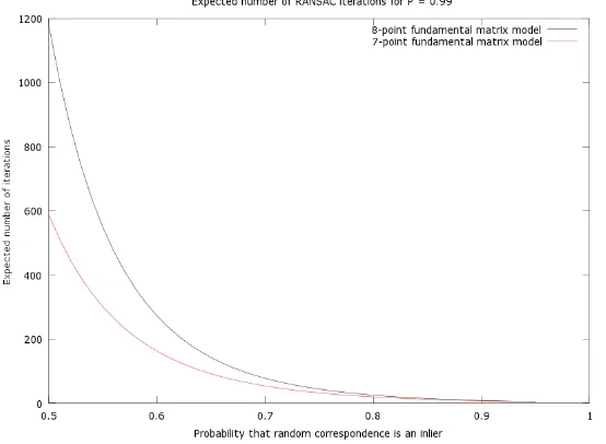
2.19 Expected RANSAC iterations for Fundamental Matrix Calculation . . . 43
2.20 RANSAC applied to SIFT correspondence . . . 44
LIST OF FIGURES xiii
2.22 Example Normal Equation Structure . . . 54
2.23 Centroid . . . 57
2.24 Common SfM Work Flow . . . 58
3.1 Downtown Rochester Point Cloud . . . 60
3.2 Software Work Flow . . . 62
3.3 Bundler Work Flow . . . 63
3.4 GPS transform . . . 65
3.5 Augmented Camera Model transform . . . 66
3.6 Direct Triangulation Method . . . 67
3.7 CAD-like surface estimation . . . 68
3.8 RANSAC Plane Fitting . . . 69
3.9 Alpha Shapes Boundary Extraction . . . 70
3.10 Object Plane Boundary Extraction . . . 71
3.11 Example Building Model . . . 72
3.12 Voxelization . . . 73
3.13 Removal of low density voxels . . . 74
3.14 Radius Search Algorithm . . . 74
3.15 Z-Level Voxel Cleaning . . . 75
3.16 Hit or Miss Transform . . . 77
3.17 Voxel Level Cleaning . . . 78
3.18 Moore-neighborhood Boundary Search . . . 79
3.19 Example Voxel Z-Level Cleaning Results . . . 81
3.20 2-D Sampling of Figure . . . 82
3.21 2-D Marching Cubes . . . 83
3.22 3-d Marching Cubes Primitives . . . 84
3.23 Example facetized surface . . . 84
3.24 Voxel Confidence Situations . . . 86
3.25 Occlusion Handling . . . 87
3.26 Generation of Depth Maps . . . 88
3.27 Extraction of structure from depth map . . . 89
LIST OF FIGURES xiv
3.29 Direct Georeferencing Process . . . 93
3.30 Ortho-map example . . . 95
3.31 Efficient Map Searching . . . 96
3.32 Facet Spectra Attribution . . . 97
3.33 Normalized Cut Example . . . 99
3.34 Region Growing . . . 101
3.35 Region Growing Clustering . . . 102
3.36 Region Growing Results . . . 102
3.37 Complete End-to-End Workflow . . . 104
4.1 SfM process with DIRSIG . . . 106
4.2 DIRSIG noiseless error . . . 108
4.3 Error in X,Y, and Z . . . 109
4.4 DIRSIG noisy error . . . 111
4.5 SfM Error . . . 113
4.6 Camera centers . . . 114
4.7 SfM Error . . . 115
4.8 Building 76 Voxel Reconstruction . . . 116
4.9 Building 7 Voxel Reconstruction . . . 117
4.10 Building 6 Voxel Reconstruction . . . 117
4.11 Building 5 Voxel Reconstruction . . . 118
4.12 Chase Tower Voxel Reconstruction . . . 119
4.13 Bausch Lomb Place Voxel Reconstruction . . . 120
4.14 Clinton Square Building Voxel Reconstruction . . . 120
4.15 Xerox Tower Voxel Reconstruction . . . 121
4.16 Confidence Histograms for RIT . . . 122
4.17 Confidence Histograms for Downtown Rochester, NY . . . 123
4.18 Thresholded Voxel Clouds . . . 124
4.19 DIRSIG simulation on extracted models . . . 125
4.20 Segmented structures from RIT dataset . . . 127
4.21 Segmented structures from downtown Rochester dataset . . . 128
LIST OF FIGURES xv
5.1 Error detection through confidence . . . 135
B.1 Graph Nodes . . . 142
B.2 Graph Cuts . . . 144
C.1 WASP Downtown Rochester Collect . . . 147
C.2 Downtown Rochester Point Cloud . . . 148
C.3 RIT Collect B . . . 149
C.4 RIT Collect Point Cloud . . . 150
C.5 Share 2010 collect over RIT . . . 151
C.6 Synthetic Image Views . . . 152
C.7 Synthetic Image Point Clouds . . . 152
D.1 Expected Output of SfM Workflow . . . 158
List of Tables
4.1 A comparison of the 95% cumulative distribution values for each georegis-tration approach between noiseless and noisy sensors . . . 110
D.1 A description of all the parameters that can be used in the RunProcess.sh script . . . 159
Chapter 1
Introduction
In recent years, with the increase of computational power and speed, many advance-ments have been made in the automation of photogrammetry through the application of computer vision methods with aerial imagery. Photogrammetry exploits the geometric properties of imagery in order to make highly accurate measurements of objects within the scene. Computer vision exploits not only the geometric properties of imagery, but also the spatial, spectral, and statistical properties with the attempt to intelligently detect and describe the objects within the imagery. Algorithms and processes in the field of analyti-cal photogrammetry developed as early as the 1960s, while computer vision evolved much later. Due to the separation in age and the difference in goals, these two fields have shared very little with each other, while their combination has significant potential.
1.1. ACCURATE STRUCTURE EXTRACTION 2
The methods required to reach theses goals can be split into two major parts. The first part is the extraction of accurate scene structure from multi-view RGB imagery. Scene structure is defined here as a collection of discrete three-dimensional measurements spread across the entire scene. These measurements form a three-dimensional point cloud, the basis for further structure modeling. Scene structure alone cannot be used to create a physically accurate three-dimensional model. The second part of the methods used in this work focus on the modeling of the extracted scene structure. The modeling process uses the scene structure along with additional scene information to estimate a physical model for specific objects within the scene.
1.1
Accurate Structure Extraction
Identifying objects within a scene is a key goal in the field of computer vision. One method of describing objects within a scene is to identify their structure through analysis of their motion between multiple images, a process commonly referred to as Structure from Motion (SfM). This technique of analyzing objects has its roots in traditional photogram-metry, though the standard goal of SfM techniques lies in object identification rather than mensuration. To that end, the SfM algorithm chain assumes little or no information about the imaging platform. The computer vision community has developed a number of com-plex processes to estimate camera pose,i.e., the sensor position and orientation, but these methods are limited to estimating parameters in a relative sense [25, 32]. Consequently, any estimated object structure is in the same relativistic coordinate system. Precise geo-graphic measurements of objects, cannot be directly extracted in this coordinate system without additional information.
1.2. PHYSICAL MODEL ESTIMATION 3
coordinate system and the desired Earth-based coordinate system can be described by a simple, seven degrees of freedom similarity transform, as they are both metric coordinate systems.
Computer vision techniques for extracting scene structure combined with additional information for geographic registration provides the required methods for extracting ac-curate scene structure from multi-view imagery. Objects contained in this scene structure can be further processed to extract physically accurate three-dimensional models.
1.2
Physical Model Estimation
Geographically accurate image-based three-dimensional structure measurements pro-vide the basis for further analysis and modeling of target objects within the scene of interest. These targets tend to be man-made structures (e.g. buildings, houses, large structures). This work focuses on the physical model estimation of these types of struc-tures.
An assumption can be made when focusing on these types of structures, more gener-ally called the “Manhattan-world” assumption [9]. This assumption is that structures in a three-dimensional Cartesian coordinate system are primarily made up of large planar faces and the structure tends to orient itself in three orthogonal directions. The original assumption stated that the camera is assumed to be approximately in the horizontal plane, having Z map with the vertical lines in the imagery. In the case of aerial imagery, the camera is assumed to be approximately orthogonal to the horizontal plane (or near the nadir viewing direction).
A voxel-based modeling process is used in this work, in order to estimate the physical model’s surface structure of a specific man-made target. Using the “Manhattan-world” assumption it can be assumed that man-made structures tend to have horizontal planes connected to vertical walls. This assumption aligns itself very well with voxel-based struc-ture modeling.
1.3. SUMMARY 4
The latter scenario is the simpler case, as all it requires is a direct mapping from the model’s surface to an atmospherically corrected hyperspectral image. When only R,G,B information is known for the scene, estimating a high resolution reflectance spectra be-comes very difficult. Instead of attempting to fully estimate the reflectance spectra for each facet on a surface model, this work looks at methods of facet classification. Given knowledge of surface classes, attempts could be made to identify the reflectance spectra through database matching. Given the large nature of that problem, this work is limited to creating methods to identify facet classes.
1.3
Summary
Physical simulation is a direct application of the automatic generation of physically accurate three-dimensional models. Three-dimensional physical simulation of imagery is the process of synthetically replicating interactions of light with three-dimensional matter and processing those interactions such that a radiometrically accurate image can be pro-duced, given a set of imaging parameters. Simulation of this nature can be very powerful for testing and analysis of novel image processing algorithms, these simulations could even be used for surveillance-based modeling. The basis for physics-based simulation, is an accurate three-dimensional model attributed with material properties. These models are painstakingly created by hand, and take many hours to complete. For this reason, this type of physical simulation is limited in the scenes it can simulate and consequently its ap-plications. Automatically creating these physical models from multi-view aerial imagery would provide a convenient method of model generation, and significantly broaden the applications of physics-based image modeling.
1.3. SUMMARY 5
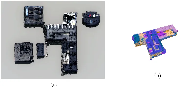
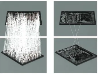
(a)
[image:22.612.124.497.127.305.2](b)
Figure 1.1: Physical modeling is performed in this work with two scenarios in mind. The first is with the addition of hyperspectral reflectance imagery, allowing for a direct mapping of spectra onto facets. This allows for physical modeling to be done easily within the spectral range of the hyperspectral imagery, a physical simulation of five structures is shown in (a). Given only R,G,B imagery, estimating the surface reflectance becomes a very difficult problem. To this end, this work attempts to classify different materials on the surface of a structure using spatial-spectral information. The classes allow for user-assisted attribution, an example of a class-mapped three-dimensional surface produced by this work is shown in (b).
Given only R,G,B imagery, estimating the surface reflectance of a model becomes an ill-posed problem. It is very difficult to discriminate between materials with such low spectral resolution sampling. Instead of identifying specific materials, potential mate-rial classes can be identified on the surface structure through analysis of the surface’s spatial-spectral properties. Figure 1.1 shows a classified three-dimensional surface created through this process. This gives the user an estimate of the structure’s surface as well as the location of different materials classes, which can be attributed by the user.
1.4. CONTRIBUTIONS 6
1.4
Contributions
The work performed here for geographically accurate structure extraction and physical model estimation makes a number of contributions. A well-known process for generat-ing geographically accurate scene structure from multi-view imagery is presented and a Linux-based, end-to-end, scripted, workflow was developed. A method for analysis of the extracted structure’s geoaccuracy was developed, and, used to evaluate the performance of several common methods for structure georegistration.
This work specifically addresses the usage of nadir-looking imagery for scene struc-ture reconstruction. Extracted strucstruc-ture from nadir imagery often contains a significant amount of noise and holes. A voxel-based noise reduction, surface estimation, and interpo-lation process is developed for estimating the surface of target objects from the extracted structure.
Chapter 2
Background
2.1. EPIPOLAR GEOMETRY 8
Figure 2.1: Structure from Motion can be broken down into a few steps: Image feature detection and matching, camera pose estimation, structure triangulation, and optimization.
Structure from Motion (SfM) provides a methodology for extracting discrete measure-ments of three-dimensional structure in a relative world coordinate system. A transform can be derived to bring the relative structure measurements to a fixed Earth-based coordi-nate system. The derivation of this transform is discussed in Section 2.5. This chapter will cover the material which is necessary to understand the three-dimensional reconstruction process used in this work, as well as review previous work done in each area. The discus-sions presented here will shed light on how an automatic three-dimensional reconstruction can be obtained.
2.1
Epipolar Geometry
2.1. EPIPOLAR GEOMETRY 9
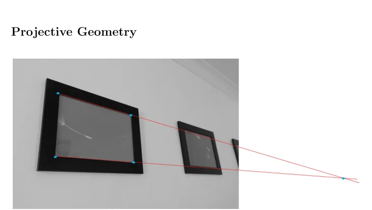
[image:26.612.156.521.151.357.2]2.1.1 Projective Geometry
Figure 2.2: Parallel lines viewed from a angled perspective often appear as though if ex-tended they will eventually intersect (this intersection point is called the point at infinity).
The notion of projective geometry has been around for centuries [23], that is, an at-tempt to quantify and model Euclidean geometry that contains a perspective view. It is a natural progression from basic Euclidean geometric modeling, since it is how humans view the world. Figure 2.2 shows a perspective view of an object on a wall. Here, there are lines within the frame that humans know to be parallel which appear to converge at some point, called the point at infinity. In order to represent this point in a coordinate system with-out causing mathematical errors, a homogeneous coordinate system is used. Projective geometry is essentially the attempt to quantify the projection of a higher-dimensional co-ordinate system onto a lower-dimensional coco-ordinate system. An example and widely used application of this is the projection of a three-dimensional scene onto a two-dimensional camera frame.
Homogeneous Coordinates
2.1. EPIPOLAR GEOMETRY 10
one extra dimension, which allows for the quantification of the projected coordinates. As an illustration, consider the algebraic definition of a line in 2-D space, shown in Equa-tion 2.1.
Ax+By+C= 0 (2.1)
The definition of a line can be vectorized by representing the line as a set of parameters A, B, and C. The vectorization of this equation is shown in Equation 2.2.
h
x y 1
i A B C
= 0 (2.2)
The left-hand vector of Equation 2.2 is considered to be a point in 2-D space, x = [x, y,1], which falls on a line in 2-D space represented by a set of parameters,l= [A, B, C]T, such that xTl = 0. The third dimension of x allows for the representation of all points that might possibly fall on linel. Parameterizingx,kx= [kx, ky, k], allows for the repre-sentation of all possible set of homogeneous points which represent the same point falling on linel, this can be seen by substituting this parametrization back into Equation 2.2,
h
kx ky k
i A B C
=k0 = 0 (2.3)
This also shows that the degrees of freedom for the homogeneous point on a line is equal to 2, the same as it would be in Euclidean space. This representation allows for a projective representation for the point x, illustrated in Figure 2.3.
The previous example gave two important properties of homogeneous coordinates in projective geometry. The first is that in homogeneous coordinates, if a pointxfalls on line
l, their dot product must be equal to zero. The second important property is the mapping from projective space to Euclidean space. For a 2-D point (x, y) the conversion is xk,yk
2.1. EPIPOLAR GEOMETRY 11
will henceforth be represented asx= [x1, x2, x3] for two-dimensional Euclidean space, and X= [x1, x2, x3, x4] for three-dimensional Euclidean space. Euclidean coordinates will be
represented using x= [x, y] and X= [x, y, z].
1 ... k
Z X Y
l
x kx
Figure 2.3: Homogeneous coordinates can be used to represent projections from higher di-mensional spaces to lower didi-mensional spaces. In this situation, the pointX can originate anywhere between the projected line and three-dimensional shape. Describing the linel in terms of homogeneous coordinates allows for the representation of all possible points which would be projected onto that line.
Homographies
A projective transformation, or homography, is defined as an invertible transformation such that x0 = H(x) [25]. The homography transforms the point x to the projective plane ofx0. For example, in Figure 2.3, a homography could be derived to transform the point x on the on the projective plane k = 1 to any projective plane k > 1. The use of homogeneous coordinates allows for a matrix representation of the function H, shown in Equation 2.4.
x01 x02 x03
=
h11 h12 h13
h21 h22 h23
h31 h32 h33
2.1. EPIPOLAR GEOMETRY 12
As shown in Equation 2.3, the parameterization of the projective space does not add a degree of freedom to the homogeneous coordinate system. Since the matrixH is defined in homogeneous coordinates, it is only defined up to this scaling factor, and therefore has eight degrees of freedom. Constraining elements of this matrix allows for affine, similarity, and Euclidean transformations to be constructed. These transformations can be useful in the manipulation of coordinate systems using homographies. The homography can be extended into higher dimensions by adding the appropriate number of rows and columns to the matrixH.
2.1.2 Camera Model
A camera can be mathematically represented as a mapping from a three-dimensional to a two-dimensional coordinate space. This can be done easily by using projective geom-etry with homogeneous coordinates.
Pinhole Camera Model
The simplest camera to model using projective geometry is the pinhole camera. Fig-ure 2.4 shows an example of a pinhole style projection of a vertical image. While the true exposure is taken at the image negative, it is more useful to define the geometry in terms of the image positive. Using similar triangles lengthsx and y can be defined as follows:
x=fXZ
y=fYZ
(2.5)
2.1. EPIPOLAR GEOMETRY 13
the principle point offset.
x=fXZ +px
y=fYZ +py
(2.6) f Z X Y x y C p
Figure 2.4: An orthogonal image projection is one where the camera frame has no rotations between the world coordinate system and the frame coordinate system. The principle point offset is included in the orthogonal image projection.
Equation 2.6 can be represented in matrix form using homogeneous coordinates. This is shown in Equation 2.7.
f X+Zpx
f Y +Zpy
Z =
f 0 px 0
0 f py 0
0 0 1 0
X Y Z 1 (2.7)
2.1. EPIPOLAR GEOMETRY 14
This can be verified by using the method for homogeneous to Euclidean coordinate con-version presented in Section 2.1.1. The projection matrix shown in Equation 2.7 is known as the camera calibration matrix,K.
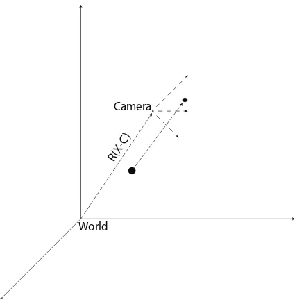
World Camera
[image:31.612.232.446.245.464.2]R(X-C)
Figure 2.5: The camera frame is often rotated relative to the world frame. In order to bring a world point into the camera frame, the point must be rotated and translated into the frame.
World to Camera Frame Transformation
2.1. EPIPOLAR GEOMETRY 15
Xcam =R(X−C) (2.8)
whereRis a 3x3 rotation matrix that rotates the world frame to the camera frame. This can be represented in homogeneous coordinates as shown in Equation 2.9.
Xcam =
"
R −RC
0 1 # X Y Z 1 (2.9)
Camera Projection Matrix
By combining the camera calibration matrix with the world-to-camera frame trans-formation, the camera projection matrix can be formed. Shown in Equation 2.10, the matrix is split into two sections, a 3x3 block representing the rotation, and a 3x1 block representing the translation. The translationt represents−RC.
P=K[R|t] (2.10)
In order to use this model with digital cameras, the camera calibration matrixKmust be modified so that the units are all the same. This requires multiplying each unit by a scale factor,m, which represents the number of pixels per unit length. The modified calibration matrix is shown in Equation 2.11.
K=
mf 0 mpx
0 mf mpy
0 0 1
(2.11)
Given Equation 2.10 combined with Equation 2.11, the relationship between a world pointX and image point xcan be defined using Equation 2.12,
x=PX (2.12)
2.1. EPIPOLAR GEOMETRY 16
2.1.3 Stereo Geometry and the Fundamental Matrix
Stereo geometry is also known as epipolar geometry. This section will cover the basic properties of epipolar geometry. Figure 2.6 shows a basic representation of two images observing the same point in space. WithC, andC0 as the camera centers,Xas the point in three-dimensional space, and the points x, and x0 as the projections of X onto their respective cameras.
C C’
X
x l x’
e e’
F P
e
Figure 2.6: Stereo (epipolar) geometry is the building block for all multi-view reconstruc-tion processes. This figure shows the posireconstruc-tions of the epipoles (e,e0), epipolar lines (l,l0), epipolar plane (P), world point (X), and camera centers (C,C0). The relationship between the imagery can be described using the fundamental matrix (F).
The three-dimensional plane made from points C, C0, andX represents the epipolar plane, Pe. Rays projected from the camera center to X are coplanar with the epipolar
plane. The intersection points of the ray between C and C0 constitute the epipoles for each image. The epipolar plane intersects each image at two points, the back projection ofXonto the image, and each image’s epipole. The epipole for each set of images remains constant for all corresponding pointsxand x0.
correspond-2.1. EPIPOLAR GEOMETRY 17
ing point in the opposing image. For example, in Figure 2.6, l0 is the image of the ray projected fromC through x. This relationship is called the epipolar line correspondence condition.
Given that there is some relationship between x and x0 using the epipolar line corre-spondence, it can be inferred that there is a homography that relates the two points.
x=Hx0 (2.13)
The cross product of x0 and e0 represents the epipolar line l0, substituting this into Equation 2.13 gives,
l=e0×Hx0 (2.14) The fundamental matrix Fhere is defined as [25],
F=e0×H (2.15)
Fundamental Matrix Properties
The fundamental matrix F, is a matrix of rank two with seven degrees of freedom. It has nine elements defined up to a single scale, which removes one degree of freedom. The fundamental matrix also satisfies the constraint,
det (F) = 0 (2.16)
which removes the last degree of freedom. The fundamental matrix has a number of properties that can be exploited for three-dimensional reconstruction. The first property comes by substituting F into Equation 2.14, which results in the algebraic definition of the epipolar line correspondence condition,
l=Fx0 (2.17)
con-2.1. EPIPOLAR GEOMETRY 18
dition. Using the line property discussed in Section 2.1.1, a relationship between a point and the epipolar line it falls on can be described using,
xTl= 0 (2.18)
Substituting Equation 2.17 into Equation 2.18 gives the equation for the correspon-dence condition,
xTFx0 = 0 (2.19)
All corresponding points between two images described by F must follow this condi-tion. This condition can be used as a model for solving for the fundamental matrix as well as using it as a model for optimization.
2.1.4 Fundamental Matrix Derivation
The fundamental matrix can be derived from two images in two ways. Each way re-quires having prior knowledge of the image properties. The first method derives the F
matrix from known image correspondences. The second method derives theFmatrix from the known camera projection matrices.
Using Correspondence
The fundamental matrix can be calculated using the correspondence condition shown in Equation 2.19. A single equation can be formed by vectorizing the fundamental matrix into a 1 by 9 vector. Doing this transforms Equation 2.19 into Equation 2.20.
x1x01f11+x1x02f12+x1f13+x2x01f21+x2x02f22+x2f23+x01f31+x02f32+f33= 0 (2.20)
Here x and x0 and represented using the x = [x1, x2, x3]T form, and making the
assumption that x3 = 1. The fundamental matrix is represented using fnm notation.
2.1. EPIPOLAR GEOMETRY 19
using values forx andx0. The form of the linear system is,
Af =
x11x
0
11 x11x
0
21 x11 x21x
0
11 x21x
0
21 x21 x
0
11 x
0
21 1
..
. ... ... ... ... ... ... ... ...
x1nx
0
1n x1nx
0
2n x1n x2nx
0
1n x2nx
0
2n x2n x
0
1n x
0
2n 1
f =0. (2.21)
Matrix Ais formed for all points 1 to n. The matrixA is of rank 8 or less, therefore, to solve for the fundamental matrix at least 8 corresponding points have to be used. A least squares solution can be found for the fundamental matrix by using singular value decomposition (SVD) [25].
SVD is an efficient way of calculating a least squares solution while constraining the solution to have a magnitude of 1. The solution is found as the right-hand singular vector in the SVD output which corresponds to the smallest singular value. In other words, if
SV D(A) =UΣVT, the solution forf is the last column of V.
Since the Fundamental matrix has only seven degrees of freedom, it is possible to estimate the matrix using seven point correspondences. The solution toAf = 0 will have a two-dimensional null space of the form,
F=αF1+ (1−α)F2 (2.22)
where the matrices F1 and F2 correspond to the last two columns of V. Using the
determinant constraint of the fundamental matrix (Equation 2.16), with Equation 2.22 the following can be created,
det (αF1+ (1−α)F2) = 0 (2.23)
The variableαcan be solved for and will have three roots. The non-complex roots can be substituted back into Equation 2.22 to solve for the matrixF. This will result in one to three possible fundamental matrices.
2.1. EPIPOLAR GEOMETRY 20
for estimation of the matrixFis discussed in Section 2.4.1.
Using Cameras
If the camera projection matrices for each image, as defined in Equation 2.12, are known, then the fundamental matrix can be derived using this information. Referring back to Figure 2.6, the world point, X, and the image point, x, are related through the camera matrix,P, as defined in Equation 2.12, which can be reformed as,
X=P†x (2.24)
Where P† represents the pseudo-inverse of the camera matrixP. The relationship of image pointx0 and X can also be defined using Equation 2.12, shown as,
x0 =P0X (2.25)
where P0 represents the camera projection matrix for the camera corresponding to the camera center C0. The world point defined in Equation 2.24 can be substituted into Equation 2.25, yielding,
x0 =P0P†x (2.26) Due to scale ambiguity, Equation 2.24 actually represents a family of possible solutions forX. This can be thought of as the ray of possible pointsX(λ) projected fromx, where
λis the unknown scale,
X(λ) =P†x+λC (2.27)
where C is the camera center of the camera associated with P. Two known points can come from this parameterization: P†x atλ= 0, andCat λ=∞. There two points can be imaged by the camera associated withP0, as,
P0P†x (2.28)
2.1. EPIPOLAR GEOMETRY 21
Using concepts discussed in Section 2.1.3, it is known that the epipolar line l0 can be defined as the cross product between the epipole e0 and the a point x0, shown in Equa-tion 2.30, using the skew-symmetric representaEqua-tion of the cross product,
l0 =
e0
×x
0 (2.30)
The epipolar e0 is the image of C, calculated with Equation 2.29. The point x0 is calculated using Equation 2.28, yielding,
l0 =P0C×P0P†x (2.31)
Using the epipolar line relationship defined in Equation 2.17, a definition for the fun-damental matrix can be derived from Equation 2.31,
F=P0C×P0P† (2.32)
This representation of the fundamental matrix can be useful when the camera projec-tion matrices are already known and the fundamental matrix is needed.
2.1.5 Relative Camera Pose Estimation
When absolute camera information is not known or available, it is possible to estimate the camera position and orientation information relative to each other using image point correspondences. This is done by using point correspondences to solve for the essential matrix and derive the camera information through matrix decomposition.
The Essential Matrix
2.1. EPIPOLAR GEOMETRY 22
essential matrix,
x0TK0−TEK−1x= 0 (2.33) It would follow that the relationship between the fundamental matrix and the essential matrix can be defined as
E=K0TFK (2.34)
In order to derive the relationship between the essential matrix and the camera pro-jection matrices, consider two cameras P and P0, as defined in equations 2.35 and 2.36. The origin ofP is the center of the world coordinate system.
P=K[I|0] (2.35)
P0=K0[R|t] (2.36)
The matricesKand K0 are the calibration matrices as defined in Equation 2.11. The matrixI is a 3x3 identity matrix. The 3x3 matrix R and the 3x1 vectort represent the rotation and translation of P0 away from P. The fundamental matrix can be derived from these two cameras as shown in Equation 2.32. The camera center for P is defined as the center of the world coordinate system, C =
h
0 0 0 1
iT
, in homogeneous coordinates. The equation for the fundamental matrix for Pand P0 is shown below (the vector0 represents a 3x1 vector of zeros).
P†=
"
K−1 0T
#
F=P0C×P0P†
F=K0−T[t]×RK−1
2.1. EPIPOLAR GEOMETRY 23
Using the relationship described in Equation 2.34, the essential matrix for P and P0
is given by,
E= [t]×R (2.38)
Equation 2.38 can be used to estimate the camera rotation and translation through matrix decomposition [25].
One important property of the essential matrix is that it is of rank two, just like the fundamental matrix. Also, the two non-zero singular values are equal to each other. This leads to the relationship [32],
EETE= 1
2tr EE
T
E (2.39)
This can be shown since the singular value decomposition ofE is E=UΛVT, where
Λis defined as,
Λ=
λ1 0 0
0 λ2 0
0 0 λ3
(2.40)
where λ1,λ2, and λ3 are the eigenvalues. All the singular values are greater than 0, the
trace ofEET can be defined as,
tr EET
=λ21+λ22+λ23 (2.41)
The left side of Equation 2.39 can be defined in terms of the SVD by,
EETE=UΛ3VT (2.42)
The n elements of Λ3 can be derived as shown below. This equation can be derived because it is known thatλ1 =λ2, and λ3= 0, for the essential matrix.
λ3n= 1 2 λ
2
1+λ22+λ23
2.1. EPIPOLAR GEOMETRY 24
Given this, Equation 2.41 can be factored out of Equation 2.42 to give,
EETE= 1
2tr EE
T
UΛVT (2.44)
Equation 2.44 is then shown to be equivalent to Equation 2.39 as E=UΛVT.
Five-Point Solution to the Essential Matrix
Using properties of the essential matrix it is possible to estimate relative camera pose using five image point correspondences. The calibrated point correspondencesqare related to the uncalibrated correspondences as shown in Equation 2.45.
q=K−1x (2.45)
The essential matrix correspondence condition in Equation 2.33 can be vectorized and reformed giving,
˜
qTE˜ = 0 (2.46)
The vectors in Equation 2.46 are vectorized in the form.
˜
q=h q1q01 q2q10 q3q10 q1q20 q2q20 q3q02 q1q30 q2q30 q3q03
i
˜
E=h E11 E12 E13 E21 E22 E23 E31 E32 E33
i
The vector˜qT can be put intoAx= 0 form by stacking the ˜qvectors for each correspon-dence, which forms a 5x9 matrix. Singular value decomposition can be used to find the null space basis vectors which solve the Ax= 0 forx. Using this, four vectors that form the basis of the right null space can be computed. These vectors, which represent E˜, can be formed back into 3x3 matrices and used to describeE in a linear combination.
E=xX+yY+zZ+wW (2.47)
2.1. EPIPOLAR GEOMETRY 25
Therefore it can be assumed that one weight can be set to any value, for simplification purposeswis set to equal 1 [11].
The constraint equation shown in Equation 2.44 can be reformulated into a system of equations which can provide a method of solving for the essential matrix. The reformula-tion is
EETE−1
2tr EE
T
E= 0 (2.48)
Given that the basis vector representation of E is of three variables, when inserted into Equation 2.48, nine cubic polynomial functions can be extracted. Each of the nine functions correspond to an element ofE. A tenth constraint can be added by using the fact that the essential matrix is rank deficient, the determinant of theEmust be equal to 0. These ten constraints form a system of ten equations which can be used to exactly solve for the scalar values of x, y and z [42]. These values, along with w = 1, are substituted back into Equation 2.47 to yield a solution for the essential matrix. The cameras rotations and translations are described in relation to the essential matrix in Equation 2.38. The following sections discuss the decomposition of the essential matrix to retrieve the rota-tions and translarota-tions.
Camera Pose Retrieval From the Essential Matrix
The essential matrix can be derived completely from a single camera’s rotation and translation as described in Equation 2.38. This can only be the case if one camera is assumed to be at the world coordinate origin, so that the second camera is described relative to the first. These cameras are shown in Equations 2.35 and 2.36. The rotation and translation of the second camera can be decomposed from the essential matrix using SVD. Given that E = UΛVT, four possible camera matrices for P0 can be derived, as shown in the following [25, 11],
P00 =
UWVT|u3
P01 =
UWVT| −u3
P02 =
UWTVT|u3
P03 =
UWTVT| −u3
2.2. FEATURE DETECTION, DESCRIPTION, AND MATCHING 26
Whereu3 represents the third column of the matrix U, and also represents the
trans-lation fromPtoP0. The matrix W is an orthogonal matrix as defined by
W=
0 −1 0 1 0 0 0 0 1
(2.50)
The equations shown in 2.49 represent four possible orientations that the camera P0
could take. P00 and P01 are related by a reverse translation along the baseline betweenP
andP0, as areP02 andP03. The camerasP00 andP02 are related by a 180 degree rotation
about the baseline [25]. Only one transformation of P0 is the correct one.
The only correct orientation of P0 is the one in which the points being viewed corre-spond to a three-dimensional point which is in front of both cameras. The other three orientations will represent a three-dimensional point which is behind one or both of the cameras. This concept is called cheirality, and can be enforced using the cheirality inequal-ities [25, 11]. Given a pair of corresponding points, a three-dimensional point,X, can be found using methods described in Section 2.3.2 withPandP00. The cheirality inequalities
state that ifX3X4<0, then the point is behind the first camera, if (P00X3)X4 <0 then
the point is behind the second camera. If both the previously mentioned inequalities are greater than zero, then the point is in front of both cameras andP00 is the correct
orienta-tion. If both the inequalities are less than zero, that corresponds to P01 and that camera
is used. If X3X4(P00X3)X4 <0, then the rotated case P02 is used, and the calculation
is done again. If the inequalities are both less than zero again, then P03 is the correct
configuration.
2.2
Feature Detection, Description, and Matching
Affine-2.2. FEATURE DETECTION, DESCRIPTION, AND MATCHING 27
SIFT is a feature detection, description, and matching algorithm which tries to add affine invariance to the SIFT algorithm, an issue that arises in wide-baseline image matching. DAISY is a method of feature description which also tries to attack the issue of wide-baseline matching. Finally, the patch-based feature detection and matching method used in the Patch-based Multi-view Stereo (PMVS) algorithm is presented.
2.2.1 SIFT
SIFT Feature Detection and Description
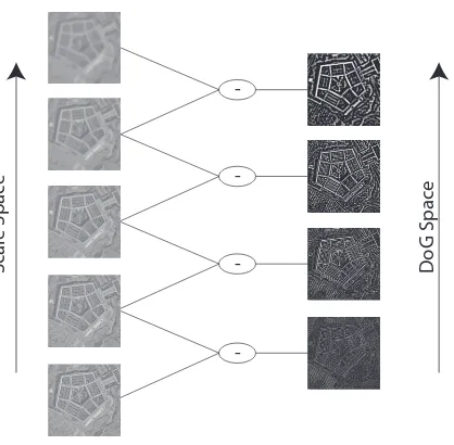
2.2. FEATURE DETECTION, DESCRIPTION, AND MATCHING 28 -S ca le Sp ac e D oG Sp ac e
Figure 2.7: SIFT calculates the position of the features in x,y, and scale space (convolved with Gaussians) for each image. This is done by taking the difference between each scale-space image. The resulting scale-space provides extrema along image edges at different scales. Features are detected within each image and between each scale.
The initial detection provides a large number of features, many of which are poor. This results since the DoG filter will provide high response along poorly defined lines, and in areas of low contrast due to noise. Poorly defined lines are detected by comparing the horizontal and vertical principle curvatures, a strong line will show low differences between principle curvatures [13]. Features along poorly defined lines as well as in low contrast areas are discarded.
In order to achieve rotational invariance, the rotation of the feature must be quanti-fied. This is done by calculating a gradient value and magnitude for each feature. The orientation and magnitude are calculated using Equation 2.51 and 2.52.
m(x, y) =
q
(I(x+ 1, y)−I(x−1, y))2+ (I(x, y+ 1)−I(x, y−1)) (2.51)
Θ (x, y) =tan−1
I(x, y+ 1)−I(x, y−1)
I(x+ 1, y)−I(x−1, y)
(2.52)
2.2. FEATURE DETECTION, DESCRIPTION, AND MATCHING 29
orientations are then formed into a thirty-six bin histogram which is used to find the dominant orientation for each feature, defined by the largest response in the histogram. For histograms with multiple maxima a separate feature is generated for each one. With knowledge of the dominant orientation and scale of each feature, the feature descriptor can be derived for each feature.
The feature descriptor is essentially a description of the orientation of the area around the detected feature. A 16-by-16 region around the feature is looked at in the scale-space of the detected feature, as shown in Figure 2.8. The grid is broken up into smaller 4-by-4 pixel regions, and an 8-bin orientation histogram is calculated for each region in the same fashion as the 36-bin orientation histogram, using Equations 2.51 and 2.52. The orien-tation is calculated relative to the dominant orienorien-tation of the feature. The histograms for each region are concatenated resulting in a scale, translation, and rotation invariant feature descriptor.
Figure 2.8: The SIFT feature is calculated over a 16-by-16 region around each detected point. The gradient direction and magnitude is calculated for each bin, the bin size is determined by the scale of the feature. The gradient angles are binned into 8-bin histograms for each 4-by-4 area, and concatenated to form a 128-element feature vector.
SIFT Feature Matching
nearest-2.2. FEATURE DETECTION, DESCRIPTION, AND MATCHING 30
neighbor matching algorithm [13]. Each SIFT feature is 128-elements in length. A dot product between each feature in one image and all the features in another image is cal-culated to determine how similar they are in a 128-dimensional space. This process can be optimized by only taking matches that are found when matching from one image to the other, and then in reverse. Figure 2.9 shows an example of two images with matching SIFT features. While this provides an estimate of feature correspondence, there is still a significant amount of error that can be removed using optimization techniques which will be discussed in Section 2.4.1.
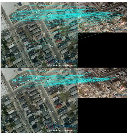
Figure 2.9: The SIFT matching process can find a very large number of matches, however, not all of the matches will be good.
2.2.2 Affine-SIFT
2.2. FEATURE DETECTION, DESCRIPTION, AND MATCHING 31
a rotation, scale, and translation invariant description of the image. The original SIFT matching process is used to match features at different tilts. Features that are matched consistently between the simulated images are kept as good matches [48]. Figure 2.10 shows an example of A-SIFT matching versus SIFT matching.
[image:48.612.170.509.345.603.2]Affine-SIFT proves to have significantly better matching results than SIFT with images that have a projective relationship. However, this comes at the expense of computational processing time [48]. Images are sub-sampled in order to speed this process up, and the algorithm can also be parallelized. The computational complexity of A-SIFT is higher than that of SIFT.
2.2. FEATURE DETECTION, DESCRIPTION, AND MATCHING 32
2.2.3 DAISY
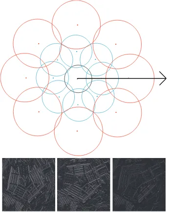
[image:49.612.253.426.321.537.2]When matching images that exhibit a large baseline, SIFT tends to have a difficult time finding correspondences [64]. As the baseline widens between the images, the trans-form that relates the two images tends to become more projective. The goal of the DAISY feature descriptor is to efficiently describe a region around every feature that is invariant to this type of transform [65]. The DAISY feature is just a descriptor, so it can be com-bined with any type of feature detector.
Figure 2.11: A representation of the DAISY feature descriptor which is applied to each orientation map. Each circle represents a Gaussian kernel with the size proportional to the Gaussian scale. The kernels radiate outwards in a set number of iterations. This feature is calculated on each orientation map. [64].
2.2. FEATURE DETECTION, DESCRIPTION, AND MATCHING 33
These maps are generated by calculating the gradient intensity in a specific direction for all chosen directions. Then each orientation map is convolved with a series of Gaussian functions of varying scale. The different Gaussian convolutions represent the scale inten-sity in each direction, thus providing a scale invariance to the descriptor. The descriptor is normalized so it can be matched between images. Figure 2.11 shows the layout of the DAISY feature descriptor. There are a number of parameters that can be altered in the descriptor. These include the radius of the whole descriptor, the number of orientation samples that are collected in each direction, the number of samples that are collected in a single orientation layer, and the number of orientation maps [64].
Invariance in the DAISY descriptor is provided by the scaling of the Gaussian functions as well as the characterization of the orientation intensities. While SIFT does attempt to quantify the orientation intensity, DAISY has proven to be a better and faster descriptor for features which differ significantly in orientation and scale [65].
2.2.4 Epipolar Line Matching
Given an initial correspondence with a feature detection and matching algorithm, such as SIFT, A-SIFT, or DAISY, the fundamental matrix can be calculated using RANSAC with the seven-point fundamental matrix algorithm, as described in Section 2.1.4. This allows for further exploitation of geometry in order to generate a denser correspondence. This dense correspondence can be used to generate a denser reconstruction. This method is based on the epipolar line constraint described in Equation 2.17. Every point in a given image will correspond to an epipolar line in the corresponding image, related by the fun-damental matrix F.
2.2. FEATURE DETECTION, DESCRIPTION, AND MATCHING 34
Figure 2.12: An example of using the epipolar line constraint along with user provided ROIs to minimize a correspondence search for two images. This search is performed between every point in the user provided ROI.
A region around the point in the original image is then matched along the epipolar line in the corresponding image. This is done by taking a 3x3 region centered around the point and vectorizing the pixels. A vector is generated for every point along the corresponding epipolar line as well as two pixels above and below the line. The vectors are matched between the two images using a brute-force matching by finding the smallest angle between the generated vectors using the dot product,
θ= cos−1
a·b
kakkbk
(2.53)
where a and b represent the vectorized regions between the two images. This process is repeated for every point in the original image’s ROI, so that every single point has a match [51].
2.2. FEATURE DETECTION, DESCRIPTION, AND MATCHING 35
in matching due to the fundamental matrix estimation. One way to reduce this error is to perform this calculation, then perform the calculation again using the corresponding im-age as the original imim-age. The correspondences which match in both directions should be kept. Figure 2.13 shows an example of one image ROI matching to a corresponding image.
Figure 2.13: A user-selected ROI being matched between an original and corresponding image. The correspondence is very dense as it was performed for every pixel in each ROI.
2.2.5 Patch-Based Model
In many SfM applications, a very dense point reconstruction is desired for modeling purposes. This process exploits epipolar geometry in a similar fashion to the one described in Section 2.2.4. This section describes the dense image correspondence method used in the PMVS algorithm described in Section 3.1. This process attempts to match every pixel within an image to another image using a patch-based region growing method, by taking advantage of epipolar geometry constraints provided by knowledge of each image camera projection matrix [18].
2.2. FEATURE DETECTION, DESCRIPTION, AND MATCHING 36
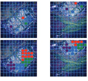
[image:53.612.167.513.259.578.2]in all directions. The filtered image is then passed to the Harris corner detector which will find only the directional changes along the detected edges. A square grid is put over the whole image, and each grid element which contains a detected local maxima is labeled as a feature. This process is shown in Figure 2.14
Figure 2.14: The PMVS feature detection and matching process; The images at the top show the image grid with initial features detected and matched using the epipolar line matching method. The images at the bottom show the expansion process in which patches are expanded and optimized based on information from the nearest reconstructed patch.
2.3. RECONSTRUCTION TECHNIQUES 37
in Section 2.1.4, the fundamental matrix between two images can be derived from their projection matrices. The epipolar line (Section 2.1.3) concept becomes useful here. Each detected feature in one image will correspond to an epipolar line in the other image. The line can be found by deriving the fundamental matrix from the known camera projection matrices as described in Section 2.1.4. The epipolar line is calculated, then all features that fall within two pixels of that line are collected. These features are considered potential matches for the original feature.
The potential matches are tested to see which features reconstruct in the best manner. The patch model is used here to determine the best reconstruction. Each feature is triangulated using the feature position and known camera information, this denotes the center of the patch. The normal to the patch is calculated as the vector between the calculated center of the patch and the known center of the corresponding camera. This normal is then compared to the vector between the calculated center of the patch, and the known center of the original camera. The vectors that differ the least, denoted by a certain qualifying threshold, are chosen to be the matching pair [18].
In order to generate a dense reconstruction, every grid element which does not contain a feature is then reconstructed by using information from the nearest reconstructed patch. The patch center and normal are initialized from the nearest reconstructed patch, and are then refined. The refining process minimizes the re-projection error between the patch center and the center of the empty image cell, by adjusting the geometric position of the initialized patch. This process produces a very dense reconstruction.
This method has proven to be extremely effective in dense reconstruction, provided that an accurate representation of a camera system can be obtained for the calculation of the camera projection matrices [18].
2.3
Reconstruction Techniques
2.3. RECONSTRUCTION TECHNIQUES 38
2.3.1 Photogrammetric Approach
For many decades the photogrammetry community have developed geometric meth-ods for triangulating three-dimensional points. These methmeth-ods are designed specifically to work with aerial imagery. An advantage that aerial images have in this process is that the camera position data is often available for each image. Therefore no prior estimation of camera positioning needs to take place. Figure 2.15 shows the basic geometry for a set of stereo images taken from an airborne platform.
Figure 2.15: The photogrammetric approach for point reconstruction uses the parallax equations. The geometry for these equations assumes that each camera’s focal plane are coplanar. It also assumes the flight line follows the x-dimension of the imagery.
2.3. RECONSTRUCTION TECHNIQUES 39
images, respectively. The following Equations 2.54, 2.55, and 2.56 describe the calcula-tions for finding the X,Y and Z coordinates. These equacalcula-tions can be derived using the similar triangles found in Figure 2.15 [73].
X = Bxl
xl−xr
(2.54)
Y = Byl
yl−yr
(2.55)
Z =H− Bf
xl−xr
(2.56)
These equations make two major assumptions about the data. The first is that the flight line is along the horizontal (x) dimension. The second assumption is that the camera focal plane is flat and level to the aforementioned flight line. Imagery taken on an aerial platform will never conform to both of these assumptions, so some coordinate modifications have to be made in order to force the data to conform to these assumptions. The flight line direction assumption can be simply corrected for by transforming the coordinate system so that the horizontal dimension falls along the recorded flight line.
2.3. RECONSTRUCTION TECHNIQUES 40
Figure 2.16: In order to compensate for the uneven focal planes, each image is projected to a new focal plane by reversing the measured pitch and roll of the aircraft, and then reorienting the x-axis for each image to be along the flight path.
The roll and pitch of the aircraft is recorded for each image frame, along with the cam-era center Using the focal length, the distance from the camcam-era center to image plane can be calculated. The new image plane is calculated using the pitch and roll of the aircraft, and the original image is projected into this new frame.
2.3.2 Linear Triangulation
This triangulation method comes from the linear manipulation of Equation 2.12. The goal of this process is to form anAX= 0 linear equation that can be solved using SVD, in the same manner that is described in Section 2.1.4. In homogeneous coordinates, the cross product of a point with itself must equal zero, given the known relationship described in equation 2.12, the following equation can be formed.
[x]×PX= 0 (2.57)
Equation 2.57 can be expanded to form three separate equations, using the definitions
x=
h
x1 x2 x3
iT
and X=
h
X1 X2 X3 1
iT
, shown here,
x1(p31X1+p32X2+p33X3+p34)−(p11X1+p12X2+p13X3+p14) (2.58)
x2(p31X1+p32X2+p33X3+p34)−(p21X1+p22X2+p23X3+p24) (2.59)
2.3. RECONSTRUCTION TECHNIQUES 41
Wherepnmrepresents nthrow and the mthcolumn of the 3x4 camera projection matrix
P. Equation 2.60 is linearly dependent on Equation 2.58 and 2.59, and for the purpose of forming a linear equation can be removed [25] The A matrix can be formed using Equations 2.58 and 2.59 as shown in Equation 2.61.
A= x1 h
p31 p32 p33 p34
iT
−h p11 p12 p13 p14
iT
x2
h
p31 p32 p33 p34
iT
−h p21 p22 p23 p24
iT
x01h p031 p032 p033 p034 iT
−h p011 p012 p013 p014
iT
x02h p031 p032 p033 p034 iT
−h p021 p022 p023 p024
iT (2.61)
Where x0n and p0nm represent a corresponding image frame. This can be formed into the linear equation shown in Equation 2.62, and solved using the SVD methods previously mentioned. x1 h
p31 p32 p33 p34
iT
−h p11 p12 p13 p14
iT
x2
h
p31 p32 p33 p34
iT
−h p21 p22 p23 p24
iT
x01 h
p031 p032 p033 p034 iT
−h p011 p012 p013 p014
iT
x02h p031 p032 p033 p034 iT
−h p021 p022 p023 p024
iT
X= 0 (2.62)
2.4. OPTIMIZATION TECHNIQUES 42
x01h p031 p032 p033 p034 iT
−h p011 p012 p013 p014
iT
x02h p031 p032 p033 p034 iT
−h p021 p022 p023 p024
iT
x11h p131 p132 p133 p134 iT
−h p111 p112 p113 p114
iT
x12h p131 p132 p133 p134 iT
−h p121 p122 p123 p124
iT
.. .
xN1 h
pN31 pN32 pN33 pN34 iT
−h pN11 pN12 pN13 pN14
iT
xN2 h
pN31 pN32 pN33 pN34 iT
−h pN21 pN22 pN23 pN24
iT
X= 0 (2.63)
This method is very simple to implement, however it is prone to error when X4 6= 1,
or requires a projective reconstruction [25].
2.4
Optimization Techniques
As with many algorithms, actual implementation of concepts requires dealing with noisy and difficult data. In the case of SfM, the feature correspondence data contains the error which needs to be minimized. Many of the previously described algorithms depend on this data as input, and are best solved using some form of optimization routine. This section will discuss some of the optimization routines which are often used to generate quality output from noisy input.
2.4.1 Feature Matching Optimization Using RANSAC
2.4. OPTIMIZATION TECHNIQUES 43
The model-fitting algorithm called RANdom SAmple Consensus (RANSAC) will be used as the optimization routine to achieve the model fitting. RANSAC is an algorithm that is designed to find the best fitting model parameters in the presence of outliers. In the feature matching case, the outliers will be the false matches. As indicated in its name, RANSAC uses a random process to iteratively find the best fitting model [17].
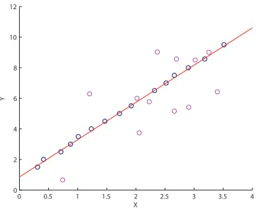
Consider a simple line fitting model, y = Ax+B, which contains two parameters; the slope A and the intercept B. This algorithm can be exactly solved with at least two data points using a least squares line fitting method. As the noise in the data increases the ability to accurately model the line using standard model fitting fails. Figure 2.17-a shows a simple least squares line fit to data which contains very little noise, Figure 2.17-b shows what happens to this least squares fit when noise is added to the system. RANSAC attempts to overcome this problem, by fitting a model to the data while simultaneously removing the outliers from the dataset.
0 0.5 1 1.5 2 2.5 3 3.5 4 0 2 4 6 8 10 12 X Y
(a) No Outliers
0 0.5 1 1.5 2 2.5 3 3.5 4 0 2 4 6 8 10 12 X Y
(b)Some Outliers
Figure 2.17: Simple linear regression can be significantly impacted in the presence of out-liers. Both lines here are fit with standard linear regression.
2.4. OPTIMIZATION TECHNIQUES 44
model within a predefined tolerance measure. This process is repeated a predefined num-ber of times until a model with enough inliers has been found or the process has repeated a set number of times.
It is important to properly set the predefined thresholds based on the input data. The distance tolerance measure can be set based on any type of assumed distribution. For example, for the line fitting algorithm, a Gaussian distributions is assumed and a distance threshold is computed. The distance measure is the square of the Euclidean distance be-tween the points, and the final distribution is a sum of squared Gaussian variables. This is modeled using aχ2DOF−1 distribution, where theDOF is equal to the number of input parameters to the model, in this case, two. The probability that a random variable is less than a given variable is modeled using the cumulative distribution function [47]. The inverse cumulative distribution function can be used to find a factor of the variance of the data, σ2, which will be used as the threshold. This is defined as,
τ =FDOF−1 −1(α)σ2 (2.64) whereFDOF−1 −1is the inverse cumulative distribution function. The probabilityαis usually chosen to be 95%, so that an incorrect rejection of an inlier only happens 5% of the time [25].
Another threshold required is the total number of expected inliers. This requires mak-ing an assumption about the proportion of the data which contains outliers. It is best to choose a conservative estimate, such as 20% or 30%. The stopping threshold can then be defined as shown in Equation 2.65 [25], whereis the assumed proportion of the data which contains outliers andnis the size of the data.
T = (1−)n (2.65)
The maximum number of samples can also be defined using probability. The proba-bility of selecting all data points within τ is wn, where w is the probability of selecting one data point within τ. To ensure with a probability of p that at least one selection, k, contains all inliers, the foll