Statistical Study of Interplanetary Coronal Mass Ejections with Strong Magnetic Fields

Rochester Institute of Technology

RIT Scholar Works

Theses Thesis/Dissertation Collections

8-13-2015

Statistical Study of Interplanetary Coronal Mass

Ejections with Strong Magnetic Fields

Matthew E. Murphy

Follow this and additional works at:http://scholarworks.rit.edu/theses

Recommended Citation

Statistical Study of Interplanetary Coronal Mass Ejections with Strong Magnetic Fields

by

Matthew E. Murphy

B.S., Seattle University, 2010

A thesis submitted in partial fulfillment of the

requirements for the degree of Master of Science

in the Chester F. Carlson Center for Imaging Science

College of Science

Rochester Institute of Technology

August 13, 2015

Signature of the Author

Accepted by

CHESTER F. CARLSON CENTER FOR IMAGING SCIENCE

COLLEGE OF SCIENCE

ROCHESTER INSTITUTE OF TECHNOLOGY

ROCHESTER, NEW YORK

CERTIFICATE OF APPROVAL

M.S. DEGREE THESIS

The M.S. Degree Thesis of Matthew E. Murphy has been examined and approved by the

thesis committee as satisfactory for the thesis required for the

M.S. degree in Imaging Science

Dr. Roger Dube, Thesis Advisor Date

Dr. Joel Kastner, Committee Member Date

Contents

List of Figures 7

Acronyms 12

Abstract 15

1 Introduction 21

2 Background and Motivation 27

2.1 Space Weather . . . 27

2.1.1 Effects of Space Weather . . . 27

2.1.3 Coordinate System . . . 33

2.2 Space Weather Prediction Center . . . 34

2.2.1 Initial parameters . . . 35

2.3 Space Weather Research Center and CCMC . . . 38

2.4 Spacecraft and Instrumentation Overview . . . 39

2.4.1 STEREOs A and B . . . 41

2.4.2 Earth directed events . . . 47

2.5 Empirical Relationships . . . 50

2.5.1 Travel time and Initial Speed Literature Review 50 2.5.2 In Situ Magnetic field and Speed Literature Review . . . 56

2.6 Problem Statement . . . 60

3 Theory 62 3.1 Relationships between solar storm parameters . . . . 62

3.1.1 Speed and Magnetic field . . . 63

3.1.3 SHARP Solar source Magnetic field . . . 64

3.2 Geoeffectiveness (and magnetic field Bz) . . . 65

3.3 CME Groups . . . 66

3.4 Summary . . . 72

4 Method 74 4.1 Plan of Study Overview and Eureqa . . . 74

4.2 Data Collection . . . 80

4.2.1 Matching ICMEs to Strong IMFs and Data Sources . . . 80

4.3 Analysis . . . 83

4.3.1 Groupings and the Magnetic Cloud Relationship 83 4.3.2 Validation of Eureqa . . . 84

4.3.3 Multi-dimensional analysis and trends using Eureqa . . . 86

5.1 Collection and Preparation of Data . . . 87

5.1.1 Collected Data Summary and Discussion . . . 91

5.2 Analysis results . . . 92

5.2.1 Groupings and the Magnetic Cloud Relationship 92

5.2.2 Validation of Eureqa . . . 97

5.2.3 Multi-Dimensional analysis: Initial CME Speed

and SHARP parameters using Eureqa . . . 101

6 Summary and Suggested Further Study 107

List of Figures

1.1 CME carrying the Sun’s magnetic field. This figure

from a space physics article by Zhou et al. (2012) . . 22

2.1 Space Weather effects. Figure is courtesy of NASA . 29

2.2 Effects of Space Weather on Satellites. Figure from a

report by D. Baker et al. (2006) [1] . . . 30

2.3 Stonyhurst Heliographic longitude and latitude

ori-entation on the Sun. Figure is from a paper by W.

Thompson [2]. . . 33

2.4 Coronagraph image observed from STEREO B.

2.5 Positions of SOHO (and ACE) and STEREO A and

B on November 24, 2009. Figure from the The Sun

Today website [3]. . . 40

2.6 STEREO A and B spacecraft and instrumentation.

Figure is from a user manual by A. Davis [4]. . . 41

2.7 Positions STEREO A and B on August 1, 2010.

Fig-ure courtesy of NASA [5]. . . 42

2.8 Positions STEREO A and B on July 1, 2012. Figure

courtesy of NASA [5]. . . 44

2.9 Positions STEREO A and B on July 1, 2014. Figure

courtesy of NASA [5]. . . 45

2.10 Positions STEREO A and B on February 18, 2015.

Figure courtesy of NASA [5]. . . 46

2.11 HARP regions on SDO/HMI imagery. From a paper

2.12 In situ Max Magnetic Field and Speed. From a paper

by Cane and Richardson [7]. . . 59

3.1 Group 1 CME example. From paper by Jian et al.

(2006) [8] . . . 68

3.2 Group 2 CME example. From paper by Jian et al.

(2006) [8] . . . 69

3.3 Group 3 CME example. From paper by Jian et al.

(2006) [8] . . . 70

3.4 Interpretive sketch of all groups. From paper by Jian

et al. (2006) [8] . . . 71

4.1 Eureqa enter data window. Screen shot from Eureqa

software [9]. . . 75

4.2 Eureqa prepare data window. Screen shot from

Eu-reqa software [9]. . . 76

4.3 Eureqa prepare data window. Screen shot from

4.4 Eureqa results window. Screen shot from Eureqa

soft-ware [9]. . . 79

5.1 Relative Locations on Sun for each event. The blue

markers are STEREO B, the orange are ACE and the

red are STEREO A. . . 90

5.2 Group 1 in 2013 max CME speed and magnetic field

at 1 AU. The line is y = 0.0362x − 1.495 with an

R2 = 0.696 . . . 93

5.3 Group 2 in 2013 max CME speed and magnetic field

at 1 AU. The line is y = 0.0375x − 3.486 with an

R2 = 0.209 . . . 94

5.4 Group 3 in 2013 max CME speed and magnetic field

at 1 AU. With a line of y = 0.0264x+ 1.134 and an

R2 = 0.165 . . . 95

5.5 Group 1 CMEs over the years 2010 to 2013. With a

5.6 The blue unfilled circles represent the Gopalswamy

ESA approximation for events with V > 500km/s

[10]. The red filled squares are the new model found

using Eureqa. Both use the speed and travel time

data seen in subsection 5.1.1. . . 100

5.7 The predicted magnetic field at ACE versus the actual

measured magnetic field. . . 103

5.8 The predicted magnetic field at ACE versus the actual

Acronyms

ACE Advanced Composition Explorer. 23

ADAPT Air Force data assimilative photospheric flux transport.

108

AU astronomical unit. 24

B magnetic field. 16

Bz Z component of the magnetic field (B). 23

CAT CME Analysis Tool. 81

CME Coronal Mass Ejection. 16

DONKI Database Of Notifications, Knowledge, Information. 81

ECA Estimated CME Arrival. 52

ESA Estimated Shock Arrival. 52

EUVI extreme ultraviolet. 39

GOES Geostationary Operational Environmental Satellites. 25

HMI Helioseismic and Magnetic Imager. 25

IMF Interplanetary Magnetic Field. 41

IMPACT In situ Measurements of Particles and CME Transients.

24

IPS interplanetary shocks. 54

nT nanoteslas. 16

PLASTIC Plasma and Suprathermal Ion Composition. 82

SDO Solar Dynamics Observatory. 25

SECCHI Sun Earth Connection Coronal and Heliospheric

Investi-gation. 24

SEP Solar Energetic Particle. 16

SHARP Space-Weather HMI Active Region Patches. 48

SOHO Solar and Heliospheric Observatory. 23

STEREO A and B Solar TErrestrial RElations Observatory Ahead

and Behind. 23

SWPC Space Weather Prediction Center. 34

WSA-Enlil Wang, Sheeley, and Arge-Sumerian god of storms and

Statistical Study of Interplanetary Coronal Mass Ejections with Strong Magnetic Fields

by

Matthew E. Murphy

Submitted to the

Chester F. Carlson Center for Imaging Science in partial fulfillment of the requirements

for the Master of Science Degree at the Rochester Institute of Technology

Abstract

Coronal Mass Ejections (CMEs) with strong magnetic fields (B)

enable the development of more accurate CME magnetic field pre-dictions and should help scientists develop better forecasts thereby helping to prevent damage to humanity’s space and Earth assets.

Acknowledgements

I would like to acknowledge my adviser Dr. Roger Dube who first

introduced me to this fascinating topic at a presentation on the 1859

Carrington event and solar storms. He also introduced me to the

software analysis tool Eureqa which was a huge part of this research.

He also provided great guidance during my studies. I’d also like to

acknowledge my committee members Dr. Joel Kastner and Dr. Tony

Vodacek. Also my contact at NASA/SWRC Dr. Yihua Zheng was

very helpful in my research and gave me the idea to study strong

magnetic field CMEs from all around the Sun. She also provided

guidance and information during weekly phone calls and emails.

Attending the Space Weather Workshop in Boulder, CO was very

helpful. While there, Captain William Frey, Captain Paul Domm,

other attendees and presenters provided lots of insight. Captain Frey

also gave me a tour of the SWPC which was very educational,

a lot of insight (so thanks also to SWPC). Also thanks to all the

members of the space weather community that helped me along the

way.

I would also like to acknowledge all the folks (faculty, colleagues

and staff) at RIT Chester F. Carlson Center for Imaging Science that

were helpful such as Cindy Schultz, Beth Lockwood and Sue Chan.

I would like to thank the US Air Force and my AF RIT colleagues

such as Captain Doug Macdonald and our AFIT CIP Liaison Officer

Major Oesa Weaver. Big thanks to Sara Smith and her Yorkshire

Terrier Kenzie. Also big thanks to my mother Teresa, father John

and brother William. Thanks to all my other family and friends that

I would like to especially dedicate this work to my mother Teresa, the

best mom ever! And also to the best dad and bro, to my father John

and my brother William. Thank you so much for always being there

Chapter 1

Introduction

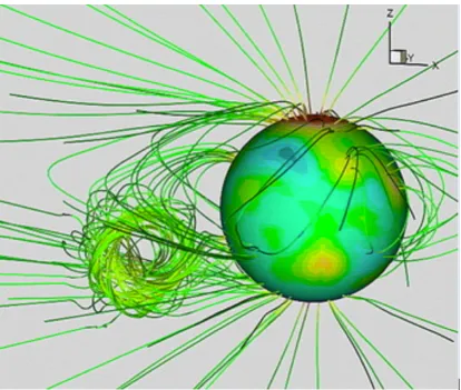
CMEs are massive solar storms that are difficult to predict. When

a CME occurs it carries with it the magnetic field of the Sun as can

Figure 1.1: CME carrying the Sun’s magnetic field. This figure from a space physics article by Zhou et al. (2012)

Earth directed CMEs and related events (SEPs and flares) can

cause severe issues to power grids on Earth, and adverse effects on

spacecraft and astronauts. Power grid issues on Earth happen when

the CME storm is geoeffective. The more geoeffective the CME, the

geoeffec-tive particularly when the magnetic field is oriented predominantly

southward (negative Bz)[12]. CMEs with southward pointing

mag-netic fields are further attracted to the Earth as they encounter the

Earth’s northward pointing magnetic field, so the effect of the storm

is not mitigated in any way as they are for CMEs with

northward-oriented magnetic fields.

Data related to CME events can be obtained from a variety of

sources. Remote sensing is used on coronagraphic images to get

pa-rameters such as speed, width and direction of these large plasma

clouds when they first emerge from the sun. A coronagraph image

can be seen in section 2.2.1 in figure 2.4. In situ measurements can

also be made at spacecraft in the path of the CMEs. The Solar

TEr-restrial RElations Observatory Ahead and Behind (STEREO A and

B) spacecraft [13] combined with the Advanced Composition

Ex-plorer (ACE) [14] and Solar and Heliospheric Observatory (SOHO)

pro-vide a 360◦ view of the sun. A Lagrangian point (as applied in this

study) is a gravitational point in interplanetary space in which a

spacecraft can orbit around. L1 is at a point between the Sun and

the Earth (at approximately 0.1 astronomical unit (AU) away from

the Earth) where the Sun’s and Earth’s gravity is balanced by the

centripetal force of the spacecraft. One AU is the distance between

the Sun and Earth.

The magnetic field strength measurements originate from

magne-tometer sensors on the ACE and STEREO spacecraft. On STEREO

A and B (described later in this thesis), the instrument is known as

the In situ Measurements of Particles and CME Transients

(IM-PACT) [13]. This IMPACT instrument also monitors SEP levels

[13]. Also on-board the STEREO spacecraft is the Sun Earth

Con-nection Coronal and Heliospheric Investigation (SECCHI)

instru-mentation. SECCHI has coronagraph cameras and extreme

from the solar source. This imagery was studied to provide the

aforementioned information about the CME source region, speed,

direction and etc. The combined capabilities of the ACE and SOHO

spacecraft at L1 can match the aforementioned capabilities of the

STEREO A and B spacecraft. Additional spacecraft and

capabili-ties for Earth directed events include the Geostationary Operational

Environmental Satellites (GOES) which can give a measure of solar

flare strength and the Solar Dynamics Observatory (SDO) spacecraft

which has the Helioseismic and Magnetic Imager (HMI) instrument

on board. The HMI instrument can give measurements of the solar

source magnetic field.

More research is needed to analyze past solar storm event

param-eters from the aforementioned spacecraft in order to better predict

and understand future solar storm events. Better prediction allows

for preventative safeguarding with minimal mission interruption of

power outages on Earth. Additionally, better forecasting of these

events will reduce solar storm related health and safety hazard risks

Chapter 2

Background and

Motivation

2.1

Space Weather

2.1.1

Effects of Space Weather

CMEs with strong magnetic fields are typically associated with SEP

can damage spacecraft, cause geomagnetic storms that can knock

out power grids on Earth, cause radio blackouts, and threaten the

health and safety of astronauts [16]. This is especially true of CMEs

with strong magnetic fields. The magnetic field strength of a CME is

linked to the strength of a geomagnetic storm on Earth, particularly

(as previously explained) when the magnetic field is predominantly

southward [12] Some of the effects of space weather can be seen in

Figure 2.1: Space Weather effects. Figure is courtesy of NASA

Space weather storms can cause multiple problems on Earth as

can be seen in figure 2.1. Spacecraft can be affected as seen in figure

Figure 2.2: Effects of Space Weather on Satellites. Figure from a report by D. Baker et al. (2006) [1]

There have been a number of storms that have hit earth. One

power issues in North America, satellites lost control and

experi-enced anomalies [18]. The Halloween storms of 2003 caused a power

outage in Sweden and interfered with satellite communications [19].

A stronger storm (which have occurred in recent history such as the

Carrington event in 1859) could cause much more damage and chaos.

If a Carrington sized event happened today, widespread power

out-ages and damage to satellites could occur, GPS could be interrupted,

the damages could cost 1 to 2 trillion dollars and the effects could

be felt for years [19].

2.1.2

CMEs, SEPs, Solar Flares and Sources

CMEs are large bursts of solar plasma from the Sun’s corona [20].

CMEs can be described by a number of parameters such as magnetic

(B) field, speed, direction, width and others. CMEs are associated

with SEPs, solar flares, and the history of their solar source regions.

the Sun sends out bursts of X-rays, gamma rays and etc. SEPs are

radiation events. Charged particles from the Sun travel on the Sun’s

magnetic field lines. There are three main kinds of solar sources:

2.1.3

Coordinate System

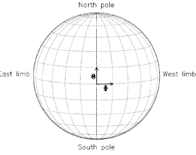
Stonyhurst Heliographic coordinate system

The coordinate system used in this paper is the Stonyhurst

Helio-graphic coordinate system. Figure 2.3 [2] gives the positive

orienta-tion of the latitude and longitude used in this coordinate system.

The solar equator and the Earth’s central meridian are at the

origin [2]. Thus, it remains fixed with respect to the Earth while the

sun rotates underneath [2]. One thing to note is that different

lati-tudes on the Sun rotate at different rates. This differential rotation

of the Sun as a function of latitude complicates the development of

models and the analysis of CME data.

2.2

Space Weather Prediction Center

The Space Weather Prediction Center (SWPC) is a 24/7 manned

op-erational center that monitors the sun. SWPC will send out warnings

when a severe Space Weather event is predicted. In order to make

these predictions, observations and measurements are taken of solar

2.2.1

Initial parameters

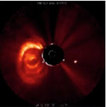
As soon as a CME becomes visible on a coronagraph the analysts

at SWPC (and other solar observatory stations) can measure the

speed, direction and width of a CME using a CME analysis tool.

The STEREO and SOHO spacecraft have coronagraph instruments

on board. A coronagraph is a telescope that has an occulting disk

in it that blocks out the bright sun (making an artificial eclipse) to

make coronal mass ejections visible. The STEREO spacecraft use

Figure 2.4: Coronagraph image observed from STEREO B. Figure courtesy of NASA.

Once the observations are made, these initial parameters are

entists Wang-Sheeley-Arge (WSA) and the Sumerian god of storms

and wind (Enlil) [23] The model consists of two parts. The first part

uses observations of the solar surface magnetic field to make an

ap-proximation of the ambient solar wind [24]. The second part consists

of inputting the initial CME parameters (speed, size, and direction)

[24].

The CME parameters are input into the existing solar wind

ap-proximation to give an estimate of the CME’s arrival time, duration

and intensity [24]. An accurate magnetic field intensity prediction

for 1 AU is not known at this time as magnetic field relationships

are an active area of research. The magnetic field of the CME is

not known until the CME passes through the ACE spacecraft at 0.1

AU away from the Earth. This distance provides only a 30 minute

warning. An example of the in situ magnetic field measurements of

a CME as it passes ACE can be seen in section 3.3 in figures 3.1

field of a CME and the initial parameters (speed, width, direction

etc.) would provide a considerably larger amount of lead-time to

space weather forecasters (and provide an additional input into the

WSA-ENLIL model).

2.3

Space Weather Research Center and

CCMC

The Space Weather Research Center (SWRC) is part of NASA and

is dedicated to improving our understanding of space weather events.

One important aspect of this center is to improve forecasting

abil-ities. SWRC is a sub-team of the Community Coordinated

Model-ing Center (CCMC) and provides space weather services to NASA

and prototypes new models, procedures and forecasting techniques

2.4

Spacecraft and Instrumentation Overview

There are a number of spacecraft whose data are considered in this

study. Each spacecraft has a suite of instrumentation on board. The

following sensors (used in this study) measure in situ parameters as

the CME passes the spacecraft: magnetic field sensors, SEP particle

flux sensors and solar wind velocity sensors. The following are

imag-ing instruments that observe the CME or the CME’s solar source

region: white-light coronagraph cameras (observe CMEs), and

ex-treme ultraviolet (EUVI) light cameras of multiple wavelengths

(serve CME source regions). Wavelengths used in this study to

ob-serve the CME solar source regions are: 193/195 ˚A (Fe XII), 304 ˚A

(He II), and 6173 ˚A (Fe I). The 193/195 ˚A (Fe XII) wavelength

ob-serves the Sun’s corona. The 304 ˚A (He II) wavelength observes the

light that is emitted from the chromosphere and transition region

on the Sun. The 6173 ˚A (Fe I) wavelength observes the photosphere

The spacecraft that provide the data used in this paper are at

various positions orbiting the sun. Figure 2.5 [3] summarizes most

of the spacecraft considered in this work.

Figure 2.5: Positions of SOHO (and ACE) and STEREO A and B

on November 24, 2009. Figure from the The Sun Today website [3].

SOHO and ACE are at L1. The positions of STEREO A and

B change relative to the Earth through out this study. Figures 2.6

2.4.1

STEREOs A and B

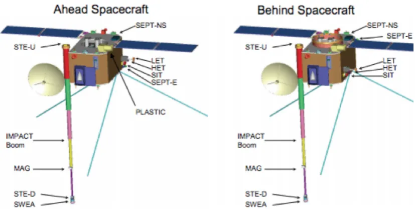
The STEREO spacecraft can be seen in figure 2.6 [4]

Figure 2.6: STEREO A and B spacecraft and instrumentation. Fig-ure is from a user manual by A. Davis [4].

The MAG instrument as seen on figure 2.6 is what detects the

Interplanetary Magnetic Field (IMF) events. STEREO A and B are

almost identical and have the same capabilities. The main purpose

of the STEREO spacecraft is to understand the three-dimensional

nature of the Sun’s corona and in particular the eruptions of the

far-side of the Sun (from such instruments as IMPACT as previously

described in chapter 1) and views of the far-side Sun (from SECCHI

also as previously described in chapter 1) previously only taken from

the Earth’s (near-side) perspective

Figure 2.7 [5] is the position of the spacecraft at the first (greater

than 30 nT) event of this study. On August 3, 2010, a greater than

30nT interplanetary magnetic field event measured at STEREO B

was also seen at the ACE spacecraft. It is interesting to note that

the ACE spacecraft did not observe a magnetic field greater than

Figure 2.8: Positions STEREO A and B on July 1, 2012. Figure courtesy of NASA [5].

Figure 2.8 [5] shows the positions of the spacecraft at roughly the

midpoint of the study. STEREO B would measure a greater than

30nT event in roughly this position. Approximately 20 days after

this point, STEREO A observed the largest magnetic field event of

Figure 2.9: Positions STEREO A and B on July 1, 2014. Figure courtesy of NASA [5].

This figure shows the positions of the spacecraft STEREO A

and B during observable events near the end of the time covered in

this study. A few months after the date of this figure, STEREO

B observed a > 30nT event. In October 2014, contact was lost

with STEREO B and the last > 30nT event at STEREO A was

due to interference because STEREO A had moved to a position in

which the Sun was near the line of sight between STEREO A and

Earth.

Figure 2.10: Positions STEREO A and B on February 18, 2015. Figure courtesy of NASA [5].

writing of this thesis paper. STEREO A at this point was in safe

mode and STEREO B has been (and still is at this point) out of

contact.

2.4.2

Earth directed events

One limitation to this study is that the STEREO A and B do not

have all the capabilities of their counterparts observing the nearside

(Earth-side) of the sun. In particular, STEREO A and B do not

have HMI or flare sensors (which are described in the next sections).

ACE

ACE is situated at L1 (see figure 2.5). It contains the

magnetome-ter sensor data that measures in situ inmagnetome-terplanetary magnetic fields

(IMF). This sensor is essentially the same as those on STEREO A

GOES

GOES are a number of weather spacecraft orbiting earth at

geosta-tionary orbits. These spacecraft provide in situ information on solar

flare intensities by measuring the flare’s X-ray flux.

SOHO

The SOHO spacecraft is at L1 (see figure 2.5). SOHO has

white-light coronagraph cameras on board which are used in conjunction

with STEREO A’s and B’s white-light coronagraph cameras to get

the initial parameters (speed, width, and etc.) of CMEs.

SDO and SHARP

SDO is at geostationary orbit. SDO has the HMI instrument on

board. Space-Weather HMI Active Region Patches (SHARPs) are

calculated from the HMI data. [6]. The SHARPs are used to measure

gradient, free energy proxy, unsigned flux and others [6]. See figure

2.11 [6].

These parameters have been used for determining the possibility

of a flare or CME occurring [6] but not used in conjunction with

coronagraphic parameters to predict B field strength at 1 AU.

2.5

Empirical Relationships

2.5.1

Travel time and Initial Speed Literature

Review

For fast CMEs (which are what are studied in this paper) the

rela-tionship found by Vandas et al. (1996) [27] was

Tshock(h) = 43–0.006Vi (2.1)

Gopalswamy [28], [29] included a relationship that involved the

effective acceleration which includes the speed at 1 AU:

a = α−βu, S = ut+ 0.5at2 (2.2)

where S is the distance traveled, u is initial CME speed near the

Sun, t is travel time, a is acceleration, and α and β are constants.

The acceleration of CMEs can be described by

a = −0.0054(u−uc) (2.3)

where uc = 406km/s is the average solar wind speed and u is the

initial speed of the CME in the coronagraph images. This is a simple

means to get the acceleration using basic kinematic relationships

[29]. This acceleration can be positive or negative depending on the

initial speed. When the CME speed is slower than the ambient solar

acceleration occurs when the CME is faster than the solar wind and

the CME is slowed due to drag. For the purposes of this study,

all accelerations are negative due to the high speeds of the studied

CMEs. Equation 2.4 is the Estimated CME Arrival (ECA) model

and is given as

t1 = −u+ √

u2 _{+ 2ad} 1

a , t2 =

d2

√

u2 _{+ 2ad} 1

(2.4)

where t is travel time, u is initial speed of a CME, a is

accelera-tion of the CME and d is distance. Usually (for slower CMEs) the

CME will slow to the speed of the solar wind at some distance d1

[30]. However, the CMEs in this study are assumed to continue to

decelerate through 1 AU due to their high initial speeds. For the

Es-timated Shock Arrival (ESA) Gopalswamy developed a relationship

for estimating speeds at 1 AU for the associated CME interplanetary

The ESA relationship is approximated as [10]

T = ABu+C (2.5)

where T is travel time, u is initial speed, A=151.002, B=0.998623

andC=11.598. This model is for CME speeds greater than 450km/s.

Wang et al. (2002) found [32]

T = 27.98 + 2.11×10

4

V (2.6)

Zhang et al.(2003) found [33]

T = 96− V

21 (2.7)

where T is travel time and V is the initial speed of the CME.

According to Zhang el al. (2003), equation 2.7 works best for CMEs

Srivastava et al. (2004) found [34]

T = 86.9−0.026V (2.8)

Manoharan et al. (2004) made a polynomial fit between travel

time in days between start time and the arrival of the interplanetary

shocks (IPS) and the initial coronagraph speed of the associated

CME. There were 91 IPS utilized in this study. Manoharan et al.

(2004) found that

tshock = 3.9−2×10−3VCM E + 3.6×10−7VCM E2 (2.9)

In a similar study by Kim et al. (2007) a linear relationship was

found [35] to be

T = 78.86−0.02VCM E (2.10)

where travel time (T) is given in hours.

How the in situ CME shock (or magnetosheath) speed and in situ

CME magnetic obstacle speed relate varies depending on the CME.

Also, the speeds vary as the CME passes the spacecraft solar wind

speed sensors. In section 3.3 in figures 3.1 thru 3.3 on pages 68 thru

70 the chart Vp on each figure shows the in situ solar wind speeds

for three types of CMEs. On each of the figures, the points from a

to b show the CME shock (or magnetosheath). The points b to c

2.5.2

In Situ Magnetic field and Speed

Litera-ture Review

In a current status of CME/shocks, Zhao and Dryer do not provide

an overview of the research of interplanetary magnetic field

predic-tions (especially their north or south polarity) due to how uncertain

they are [30]. This is one indication that more research into IMF

predictably is required. The geoeffectiveness of a CME is largely

de-termined by the magnetic polarity of the CME so more information

on this is of great value to space forecasters (see section 3.2).

Gonzalez et al.(1998) found that magnetic cloud CMEs in situ

magnetic field correlated to the in situ CME max speed and is given

as

|B|max(nT) = 0.047Vmax(km/s)−1.1 (2.11)

Equation 2.11 uses data from events directed only at Earth. A

temper-ature, has increased magnetic field, and has a smooth and rotating

magnetic field direction as observed by in situ spacecraft. [36]. A

Considering a number of CME events directed only at the ACE

spacecraft (and Earth) Owens and Cargill developed an empirical

relationship which is described by

|B|max(nT) = 0.047Vmax(km/s) + 0.0644 (2.12)

where V is the initial maximum speed of the CME and B is the

maximum observed in situ magnetic field. No consideration was

made for magnetic cloud and non-cloud events. Events were included

that had a greater than 18nT magnetic field at ACE for 3 hours or

Cane and Richardson compared max magnetic fields and speeds

from 1996 to 2009 as can be seen in figure 2.12 [7].

Figure 2.12: In situ Max Magnetic Field and Speed. From a paper by Cane and Richardson [7].

The equation of the magnetic cloud line is

Bmax(nT) = 0.0439V −1.8019 (2.13)

The equation of the non-cloud line is

From figure 2.12, the correlation coefficient found for magnetic

field (cc = 0.600) correlated to the in situ max speed much better for

cloud than for non-cloud CMEs (cc = 0.277). The Eureqa program

(which is explained in section 4.1) will be used to fit a linear trend

to the same data found in figure 2.12. Eureqa is validated by

com-paring the correlation coefficients found by Eureqa to the correlation

coefficients found by Cane and Richardson.

2.6

Problem Statement

The arrival time and strength of strong B field CME events are

difficult to predict; this prediction is critical in preventing possible

damage to people, infrastructure, and technological instrumentation.

The current correlations between strong B field events and other

so-lar parameters are not well understood. This work will lead to a

would be very useful to space weather forecasters if a correlation can

be made between Bz and any of the other solar storm parameters

Chapter 3

Theory

3.1

Relationships between solar storm

parameters

The size of the in situ magnetic field strength should be related to the

other parameters of a particular CME. In situ magnetic field strength

is the B field measured by magnetometer instruments on the ACE

be seen in figure 3.1 in section 3.3.

3.1.1

Speed and Magnetic field

As shown in section 2.5.2, there is a relationship between the in situ

speed of the CME and the in situ magnetic field.

3.1.2

Distance, Time, velocity and acceleration

As seen in equation 2.2 in chapter 2 the kinematic equation

(repro-duced here again as equation 3.1 for readability) is given as

S = ut+ 0.5at2 (3.1)

where the distance (S) is approximately 1 AU for all three

space-craft (ACE and STEREOS A and B), t is travel time, u is initial

speed of the CME, and a is acceleration.

a software data analysis tool (Eureqa) used in this study which is

further explained in section 4.3.2. Using Eureqa, a relationship is

found using data for CME coronagraph initial speed and CME travel

time. As seen in chapter 5, Eureqa is able to find the acceleration

relationship as seen in equation 3.1. Eureqa is described in section

4.1

3.1.3

SHARP Solar source Magnetic field

Unsigned flux

Bobra et al. (2014) provide a definition for a parameter known as

unsigned flux in units of Maxwells (Mx) [6] and is given as

Φ = Σ|Bz|dA (3.2)

It makes intuitive sense that the Bz at the CME solar source should

Another parameter from Bobra et al. (2014) is known as the

horizontal gradient of the horizontal field and is units of Gauss per

mega-meter (GM m−1) [6] and is given as

|Bh| =

1

NΣ

s

(∂Bh

∂x )

2 _{+ (}∂Bh ∂y )

2 _(3.3)

This parameter is related to total magnetic field in chapter 5.

3.2

Geoeffectiveness (and magnetic field

B

)

The main driver of the geoeffectiveness of the CME storm on Earth

is negative Bz, although high solar wind speed can also be a factor

[12]. A CME with a negative (or southward) Bz is more geoeffective

because the southward Bz couples with Earth’s northward pointing

magnetosphere. The strength of the negative Bz is not known until

this does not bring much lead time (only about 30 minutes). If

a correlation can be made between Bz and any of the other solar

parameters that would be very useful to space weather forecasters.

3.3

CME Groups

Jian et al.(2006) describe three different types of CME groups [8].

These groups are based on the in situ measurements of pressure

ver-sus time. Group 1 CMEs are classified as CMEs in which the

pres-sure in the magnetosheath of the CME increases gradually, Group

2 remain at a relatively stable value, and Group 3 increase quickly

and then fall off. Each group can be seen in figures 3.1, 3.2 and 3.3

for group 1,2 and 3 respectively [8]. The bottom chart of each figure

shows pressure versus time (Pt). Also included areBx/B,By/B, and

Bz/B which are the x, y and z magnetic field with total magnetic

beta. Group 1 CMEs are usually associated with magnetic clouds

and tend to have similar traits [8]. Utilizing the Jian et al. (2006)

group identification is superior to using the cloud and non-cloud

identification in that group identification has a geometric physical

meaning and is also easier to work with (since only one type of in

situ observation is considered instead of three). Furthermore, the

Figure 3.4 shows an interpretive sketch of the geometry of the

groups [8].

As shown in chapter 2 in situ magnetic field and in situ speed

have been related based on whether the CME exhibited traits of

a magnetic cloud. Using STEREO data organized into groups from

Jian et al.(2013) [37] over the years of 2010 to 2013, the in situ speed

and magnetic field relationship based on these groups was explored

as shown in chapter 5.

3.4

Summary

It has been shown in subsection 2.5.1 on page 50 that the initial CME

speed can be correlated to the in situ CME speed due to acceleration.

Furthermore, it has been shown in subsection 2.5.2 on page 56 that

the in situ speed at 1 AU can be related to the in situ magnetic field.

The speed at 1 AU is related to the initial (coronagraphic) speed

(by acceleration), thus the in situ magnetic field and initial speed

be related in some way. By matching a CME’s source magnetic field

information, speed (from coronagraphic observations) and the in situ

magnetic field observations of those same CMEs one should be able

to correlate to make a prediction of the 1 AU magnetic field. Using a

multidimensional analysis software (Eureqa) a prediction model for

in situ magnetic field of CMEs using solar source magnetic field and

Chapter 4

Method

4.1

Plan of Study Overview and Eureqa

Eureqa is a sophisticated analysis tool that can find previously

un-known correlations and relationships between various data variables.

This tool is potentially very valuable in developing empirical

The first step in using Eureqa is to enter tabulated data into the

program with each variable as a single column and provide a name

for each variable. See figure 4.1

The data can then be prepared before analysis by removing

out-liers or missing values. See figure 4.2

Next, a model target is set by describing which variables are

independent or dependent. Additionally, a relationship between the

variables can be entered into the model target. See figure 4.3

Figure 4.3: Eureqa prepare data window. Screen shot from Eureqa software [9].

Next the program is started by the user and Eureqa then

au-tomatically discovers models from the given data using algorithms

that are evolutionary and sophisticated [38]. Eureqa uses symbolic

finding equations to fit to the given data [39].

Once the Eureqa program has been run, different models found by

the program can be viewed and the user can select the best model/s

Figure 4.4: Eureqa results window. Screen shot from Eureqa soft-ware [9].

In order to validate Eureqa’s use for solar storm CME

literature were found using Eureqa and CME data. Once Eureqa

was shown to reproduce relationships found in literature, other new

relationships were explored.

4.2

Data Collection

4.2.1

Matching ICMEs to Strong IMFs and Data

Sources

The CME data collection began by first finding in situ magnetic

fields above the 30 nT threshold from the ACE and STEREO

space-craft. For comparison the Earth’s magnetic field is about 1000 times

stronger than this threshold. Magnetometer instruments on each

spacecraft provided this data. This study was done from 2010 to

October 2014 (until the STEREO data became unreliable or

unavail-able, see chapter 2). On the STEREO spacecraft this instrument is

was most likely the cause of these events was found; this data can

be seen in chapter 5 in table 5.1. The CME list from the NASA

Space Weather Database Of Notifications, Knowledge, Information

(DONKI) site [40] was used for this. This site provided a speed,

time, width and sometimes a solar source location.

The speed, width and etc. were found by space weather

forecast-ers using the STEREO SOHO CME Analysis Tool (CAT) [41]. This

tool uses three dimensional projection (from the three spacecraft) to

get accurate speeds, widths and etc. The speed, width and

direc-tion of each CME is shown on table 5.2. Addidirec-tionally, informadirec-tion

regarding an accompanying solar flare was sometimes provided. In

addition to the information about the magnetic field the strength of

any SEP event was also collected (from the IMPACT instrument).

The source location of the CME was found by forecasters (and by

the author if not available) by using the extreme ultraviolet light

loca-tions on the Sun can be seen in chapter 5 in figure 5.1. In addition

to the speed near the Sun (within 30 Solar Radii) the solar wind

speed at (or near) 1 AU was also gathered using the Plasma and

Suprathermal Ion Composition (PLASTIC) instrument [42].

A table used for reference and comparison to the NASA CCMC

DONKI site is updated on another NASA site [43]. The full catalog

is described by Gopalswamy et al (2009).[21]. This site provided

information on a subset CMEs and is useful because it also includes

backside CMEs (not just those directed at Earth) many of which

are those that were selected as mentioned previously. This table

includes CME coronagraph and solar source location information

among other things.

Another table used for reference is found online at a Caltech

website [44]. This catalog only includes ACE in situ measurements

but is useful in that in provides information as to whether the CME

and Richardson [7].

A table that was used for a separate analysis and reference is

updated on a UCLA website [45]. This table is discussed by Jian et

al.(2013)[37]. This table has STEREO CME event in situ

measure-ments from 2006 to December 2013 for Behind and to June 2014 for

Ahead. It includes what group each event belongs to as described

in section 3.3. It also has max in situ magnetic field, in situ

pres-sure, in situ solar wind speed measurements and some other CME

parameters.

4.3

Analysis

4.3.1

Groupings and the Magnetic Cloud

Rela-tionship

Jian et al. (2006) pointed out that group 1 CMEs as compared to

most features with magnetic cloud CMEs [8]. The data catalog as

described by Jian et al.(2013) with in situ STEREO event

informa-tion was used to compare max magnetic field and max solar wind

speed of the CME events from 2010 to 2013 (same time period has

the selected CME events) [37]. The magnetic field and speed

rela-tionship is described in subsection 2.5.2 and is supported by Owens

et al.(2002) [46], [47] and others. It will be investigated to see how

Group 1, 2 and 3 max speed at 1 AU compares to the magnetic field

at 1 AU measurements.

4.3.2

Validation of Eureqa

As described in section 4.1, Eureqa is a useful data analysis tool.

However, it is important to first validate Eureqa to see if it can find

the relationships already described in literature. The data from the

figures 2.12 in subsection 2.5.2 was run using Eureqa to verify that

the trend found using Eureqa for this paper’s data set for velocity

and travel time is compared to the ESA shock model described by

Gopalswamy et al.(2005) [10]. The trend to be used is similar to

equation 3.1 and is known as the kinematic relationship.

Rewrit-ing equation 3.1 from page 63 in preparation for use in the Eureqa

program:

a

t = u+bu

c_{t (4.1)}

where u is initial speed of the CME, t is travel time of the CME,

a, b and c are constants to be found using Eureqa. This equation

relates distance, time, speed and acceleration. The variables u and

t are from STEREO and ACE data over 2010 to 2014 as described

4.3.3

Multi-dimensional analysis and trends

us-ing Eureqa

The validation of Eureqa’s capabilities is presented in section 5.2.2.

Once the Eureqa software [9] had been validated, three dimensional

relationships were explored. Variables such as magnetic field at the

solar source, speed near the sun and in situ magnetic field were

Chapter 5

Results and Discussion

5.1

Collection and Preparation of Data

Tables 5.1 and 5.2, show the CME data collected for this thesis.

Table 5.1 shows which CME was matched to each in situ CME

mag-netic field measurement. Table 5.2 shows the details of the CMEs

from table 5.1.

The relative locations on the Sun for each of the greater than

Table 5.1: IMF max in situ measurement with corresponding iden-tified CMEs

IMF Date IMF Time, UT Spacecraft Max B(nT) CME date CME time

8/3/10 4:59 Behind 33.9 8/1/10 8:20

2/17/11 23:53 ACE 31.6 2/15/11 1:56

8/5/11 17:06 ACE 36.1 8/2/11 5:19

9/24/11 9:03 Behind 34.3 9/22/11 11:24

9/26/11 11:50 ACE 34.6 9/24/11 12:33

10/3/11 22:23 Behind 35.1 10/1/11 20:48

1/22/12 5:14 ACE 31.1 1/19/12 15:10

1/24/12 14:21 ACE 36.3 1/23/12 4:00

1/29/12 13:04 Ahead 49.6 1/27/12 16:39

3/8/12 10:42 ACE 40.6 3/7/12 0:36

3/19/12 23:37 Ahead 35.3 3/18/12 0:39

3/28/12 21:37 Behind 37.3 3/26/12 23:12

5/28/12 2:48 Ahead 45.4 5/26/12 22:54

6/16/12 8:56 ACE 41.6 6/14/12 12:52

7/4/12 6:56 Behind 40.5 7/2/12 8:36

7/23/12 21:00 Ahead 109.4 7/23/12 2:36

9/23/12 9:20 Behind 30.6 9/20/12 15:24

5/16/13 9:42 Ahead 30.3 5/13/13 17:24

7/25/13 6:28 Ahead 41.8 7/22/13 6:24

10/2/13 1:17 ACE 32.7 9/29/13 20:39

10/8/13 19:37 ACE 35.8 10/6/13 14:39

11/6/13 1:52 Behind 31.3 11/4/13 5:09

3/14/14 23:00 Behind 29.3 3/12/14 14:39

7/1/14 11:20 Behind 33.3 6/29/14 12:39

9/12/14 15:21 ACE 31.7 9/10/14 18:18

9/25/14 14:09 Behind 68.9 9/22/14 9:12

Table 5.2: Initial parameters of CMEs identified as seen in table 5.1

CME date CME time CME Speed (km/s)

Direction

(LON/LAT) Width

8/1/10 8:20 1000 -34/24 96

2/15/11 1:56 900 0,-20 70

8/2/11 5:19 900 15/4 35

09/22/11 11:24 1000 -90/10 140

9/24/11 12:33 1507 -45/12 100

10/1/11 20:48 1500 -120/20 90

1/19/12 15:10 1020 -21/46 138

1/23/12 4:00 2211 26/41 62

1/27/12 16:39 2200 75/40 110

3/7/12 0:36 2200 -60/30 100

3/18/12 0:39 1450 105/25 120

3/26/12 23:12 1450 -105/15 100

5/26/12 22:54 1650 -110/5 70

6/14/12 12:52 1364 -9/-20 100

7/2/12 8:36 1100 -130/-10 70

7/23/12 2:36 3400 138/-10 160

9/20/12 15:24 2319 -138/-28 112

5/13/13 17:24 1050 80/10 72

7/22/13 6:24 1000 157/30 70

9/29/13 20:39 1100 8/26 70

10/6/13 14:39 790 6/-15 50

11/4/13 5:09 1950 -178/-25 134

3/12/14 14:39 1150 -154/30 120

6/29/14 12:39 750 138/-10 60

9/10/14 18:18 1400 10/15 45

9/22/14 9:12 795 -165/13 92

Sun is for illustrative purposes only. It is a 360◦ Stonyhurst

com-posite map of EUVI/AIA 304 ˚A images taken from STEREO A,

STEREO B and ACE on November 14, 2013.

Figure 5.1: Relative Locations on Sun for each event. The blue mark-ers are STEREO B, the orange are ACE and the red are STEREO A.

On figure 5.1 it is important to note that the STEREO A events

get progressively further west (positive HEEQ) and the STEREO

pro-gressives. Also note that all the source locations are within +/- 30◦

latitude from the solar equator.

5.1.1

Collected Data Summary and Discussion

All CME events in this study had initial speeds above 750km/s.

Additionally, 88% of the events studied had associated SEP events.

One event that stands out as being odd is the 68.9 nT at STEREO

B which occurred on September 25, 2014. This event had one of

the slowest CME speeds for this data group (795km/s) and yet the

second highest magnetic field measurement. It may be that

mea-surement took into account multiple CMEs and not just the one it

5.2

Analysis results

5.2.1

Groupings and the Magnetic Cloud

Rela-tionship

Groups 1, 2 and Group 3 CMEs during 2013 were compared using

the max CME magnetic field and max in situ CME speed from the

database from Jian et al. (2013) [37]. Figures 5.2 thru 5.4 show

Figure 5.2: Group 1 in 2013 max CME speed and magnetic field at

Figure 5.3: Group 2 in 2013 max CME speed and magnetic field at

Figure 5.4: Group 3 in 2013 max CME speed and magnetic field at

Figure 5.5: Group 1 CMEs over the years 2010 to 2013. With a line

of y = 0.0326x−0.4253 and a R2 = 0.452.

Equation 5.1 below shows the magnetic cloud trend found by

Cane and Richardson [7] (on the left) and that found using group 1

data (on the right). These equations show that the magnetic cloud

These groups proposed by Jian et al.(2006) [8] could prove useful for

1 AU magnetic field prediction. The two equations are given as

Bmax,M C(nT) = 0.0439V −1.8019, Bmax,1(nT) = 0.0326V −0.4253 (5.1)

The Group 1 correlation coefficient of the best fit trend (cc =

0.672) is better than correlation coefficient found by Richardson et

al. (2010) (cc = 0.600) [7].

5.2.2

Validation of Eureqa

Validation of Magnetic fields and speed

Eureqa was validated using the method described in chapter 4 and

The cloud CME equation was found to be

B = 0.0403V −0.903 (5.2)

whereB is magnetic field and V is in situ speed of the CME. The

Eureqa program found a correlation coefficient ofcc = 0.638 which is

better than that found by Richardson et al. (2010) (cc = 0.600)[7].

The non-cloud CME equation was found to be

B = 0.0187V + 3.184 (5.3)

The Eureqa program found a correlation coefficient ofcc = 0.332

which is actually again better than that found by Richardson et al.

Validation of Travel time and speed model

The new speed and travel time model found using the Eureqa tool

[9] is

31997.7

T = V −7.79×10

−6_{T V}1.997 _(5.4)

where T is CME travel time and V is initial speed.

Solving equation 5.4 for T we have

T = 6.418×10−41.000×10

8_{V −6324}√_2.500×108_V2_−2.492×108_V1.997

V1.997 (5.5)

The new speed and time model found using Eureqa and the data

as found in subsection 5.1.1 is compared to the Gopalswamy ESA

Figure 5.6: The blue unfilled circles represent the Gopalswamy ESA

approximation for events with V > 500km/s [10]. The red filled

squares are the new model found using Eureqa. Both use the speed and travel time data seen in subsection 5.1.1.

As can be seen by figure 5.6 the two models are very similar.

The empirical Eureqa model however is more easily explained

phys-ically than the Gopalswamy ESA approximation model because the

Eureqa equation came directly from the kinematic relationship as

shown in chapter 3 in equation 3.1. In contrast, the Gopalswamy

proven it can be given a set of CME data and find the physical

relationship that relates the CME data parameters.

5.2.3

Multi-Dimensional analysis: Initial CME

Speed and SHARP parameters using

Eu-reqa

Using the freshly validated tool, Eureqa was then applied to study

various solar source SHARP magnetic field parameters for possible

correlation use in 1 AU (at ACE) magnetic field prediction. Two

pa-rameters that stood out as possible predictors were (1) the unsigned

flux (Φ) for the Bz 1 AU prediction and (2) the mean magnetic field

horizontal gradient(|Bh|) for the 1 AU total magnetic field (B)

pre-diction. These parameters stood out due to their high correlation to

the parameters of interest. These parameters were combined with

the initial speed of the CME to create models to predict magnetic

The empirical model found to predict total magnetic field (B) is

B = 28.51 + 0.00389V + 1.79

|Bh| −56.56

(5.6)

where V is the initial speed of the CME and |Bh| is mean magnetic

field horizontal gradient. This equation is compared to the actual

B and this comparison is shown in figure 5.7. Eureqa’s ability to

predict observables (“predicted”) should appear as a straight line

with reasonable correlation coefficients when compared to the actual

Figure 5.7: The predicted magnetic field at ACE versus the actual measured magnetic field.

The fit of the line in figure 5.7 is

y = 0.324x+ 22.77 (5.7)

this trend line has a R2 = 0.406. The mean of the differences

deviation is 2.86.

The empirical model found to predict minimum Bz is

Bz = 0.00764V −20.58−1.97×10−22Φ (5.8)

where V is the initial speed of the CME and Φ is the unsigned

flux. This equation is compared to the actual predicted Bz and this

Figure 5.8: The predicted magnetic field at ACE versus the actual measured magnetic field.

The fit of the line in figure 5.8 is

y = 0.5664x−7.1073 (5.9)

This line has an R2 = 0.60606. The mean of the differences

deviation is 3.36.

Relationships 5.8 and 5.6 can be understood from a physics

per-spective in that the magnetic field source information describes how

much potential energy is on the sun. Additionally, the speed

rep-resents how much of that energy escapes the sun. When these

pa-rameters are combined as done in this work, the CME magnetic

field strength can be predicted. This can dramatically increase the

lead time (from approximately 30 minutes to approximately a day

or more) for CME magnetic field prediction; in other words instead

of waiting for the CME to get close to Earth a prediction can be

made close to the Sun.

Other parameters were investigated but not included in this

the-sis due to the complexity required in the interpretation, or the

use-fulness and low-impact of these other parameters. Such parameters

were the SEP proton flux, the solar flare flux, the area of the NOAA

Chapter 6

Summary and

Suggested Further

Study

The groups proposed by Jian et al. (2006) [8] have been shown in

this paper that they can be used in relating in situ magnetic field

Owens et al. (2002) [46], [7].

Using Eureqa, previously unknown functional relationships

be-tween solar storm parameters were found by relating SHARP solar

source magnetic field parameters and coronagraph CME speed to

CME 1 AU magnetic field data. Up to now (as shown in chapter

2) SHARP data has only been used for the prediction of the

prob-ability of a flare or CME event occurring on a certain part of the

Sun. Now, SHARP data has been shown that it can be used for 1

AU CME magnetic field prediction. The relationships found using

Eureqa were given to the SWRC and could potentially be very useful

to the SWPC and other space weather forecasters.

For this study it was unfortunate that HMI/SDO SHARP data

was only available for Earth facing events. Future study could

in-volve the Air Force data assimilative photospheric flux transport

(ADAPT) model [48]. ADAPT provides far side magnetic field

al-teration to the SHARP code in order to calculate far-side HARP

regions from these maps. From this, far side magnetic field

param-eters would be generated. These paramparam-eters (with the knowledge

of CME STEREO source locations) could then be correlated to the

STEREO CME parameters to see if the relationships found at ACE

still hold true (as seen in chapter 5). Additionally, other solar storm

parameters could be investigated. For instance, instead of predicting

the CME magnetic field, the amount of X-ray flux from solar flares

Chapter 7

Bibliography

[1] D. Baker, L. Barby, S. Curtis, J. Jokipii, W. Lewis, J. Miller,

W. Schimmerling, H. Singer, L. Townsend, R. Turner, et al.,

“Space Radiation Hazard and the Vision for Space Exploration:

Report of a Workshop,” 2006.

[2] W. Thompson, “Coordinate Systems for Solar Image Data,”

Astronomy & Astrophysics, vol. 449, no. 2, pp. 791–803, 2006.

thesuntoday.org/tag/cor1/.

[4] A. Davis, “STEREO IMPACT SEP Sensor Suite Commanding

and Users Manual.” http://www.srl.caltech.edu/STEREO2/

docs/SEP_CommandingUserManual_J.pdf.

[5] J. Gurman, “Where is STEREO Today?.” http:

//stereo-ssc.nascom.nasa.gov/where.shtml.

[6] M. G. Bobra, X. Sun, J. T. Hoeksema, M. Turmon, Y. Liu,

K. Hayashi, G. Barnes, and K. Leka, “The Helioseismic

and Magnetic Imager (HMI) vector magnetic field pipeline:

SHARPs–space-weather HMI active region patches,” Solar

Physics, vol. 289, no. 9, pp. 3549–3578, 2014.

[7] I. Richardson and H. Cane, “Near-Earth Interplanetary Coronal

Mass Ejections during Solar Cycle 23 (1996–2009): Catalog and

Summary of Properties,” Solar Physics, vol. 264, no. 1, pp. 189–

[8] L. Jian, C. Russell, J. Luhmann, and R. Skoug, “Properties of

Interplanetary Coronal Mass Ejections at one AU during 1995–

2004,” Solar Physics, vol. 239, no. 1-2, pp. 393–436, 2006.

[9] M. Schmidt and H. Lipson, “Eureqa (version 0.98

beta)[software],” 2013.

[10] N. Gopalswamy, S. Yashiro, Y. Liu, G. Michalek, A. Vourlidas,

M. Kaiser, and R. Howard, “Coronal Mass Ejections and other

extreme characteristics of the 2003 October–November Solar

Eruptions,” Journal of Geophysical Research: Space Physics

(1978–2012), vol. 110, no. A9, 2005.

[11] Y. Zhou, X. Feng, S. Wu, D. Du, F. Shen, and C. Xiang, “Using

a 3-D Spherical Plasmoid to Interpret the Sun-to-Earth

Propa-gation of the 4 November 1997 Coronal Mass Ejection Event,”

Journal of Geophysical Research: Space Physics (1978–2012),

[12] E. Kilpua, Y. Li, J. Luhmann, L. Jian, and C. Russell, “On

the Relationship between Magnetic Cloud Field Polarity and

Geoeffectiveness,” in Annales Geophysicae, vol. 30, pp. 1037–

1050, Copernicus GmbH, 2012.

[13] J. Luhmann, D. Curtis, P. Schroeder, J. McCauley, R. Lin,

D. Larson, S. Bale, J.-A. Sauvaud, C. Aoustin, R. Mewaldt,

et al., “STEREO IMPACT investigation goals, measurements,

and data products overview,” Space Science Reviews, vol. 136,

no. 1-4, pp. 117–184, 2008.

[14] K. Erickson, “ACE.” http://science.nasa.gov/missions/

ace/.

[15] K. Erickson, “SOHO.” http://science.nasa.gov/missions/

soho/.

[16] V. Bothmer and I. A. Daglis, Space Weather: Physics and

[17] J. Rumburg, “Solar Storm and Space Weather.” http:

//www.nasa.gov/mission_pages/sunearth/spaceweather/

#.VJTLvF4AKA.

[18] S. Odenwald, “The Day the Sun Brought Darkness.”

http://www.nasa.gov/topics/earth/features/sun_

darkness.html.

[19] R. Lovett, “What If the Biggest Solar

Storm on Record Happened Today?.” http:

//news.nationalgeographic.com/news/2011/03/

110302-solar-flares-sun-storms-earth-danger-carrington/.

[20] A. Hundhausen, “Coronal Mass Ejections,” in The Many Faces

of the Sun, pp. 143–200, Springer, 1999.

[21] N. Gopalswamy, S. Yashiro, G. Michalek, G. Stenborg, A.

Catalog,” Earth, Moon, and Planets, vol. 104, no. 1-4, pp. 295–

313, 2009.

[22] “STEREO CME Analysis Tool.” http://ccmc.gsfc.nasa.

gov/analysis/stereo/.

[23] C. Bailey, “What is the WSA-ENLIL Model?.” http://swc.

gsfc.nasa.gov/main/enlilvideo.

[24] A. Parsons, D. Biesecker, D. Odstrcil, G. Millward, S. Hill, and

V. Pizzo, “Wang-Sheeley-Arge–Enlil Cone Model Transitions to

Operations,” Space Weather, vol. 9, no. 3, 2011.

[25] M. Mays, A. Taktakishvili, A. Pulkkinen, P. MacNeice,

L. Rast¨atter, D. Odstrcil, L. Jian, I. Richardson, J. LaSota,

Y. Zheng,et al., “Ensemble Modeling of CMEs Using the WSA–

ENLIL+ Cone Model,” Solar Physics, pp. 1–40, 2015.

[26] A. Chulaki, “Community Coordinated Modeling Center.”http:

[27] M. Vandas, S. Fischer, M. Dryer, Z. Smith, and T. Detman,

“Parametric Study of Loop-like Magnetic Cloud Propagation,”

Journal of Geophysical Research: Space Physics (1978–2012),

vol. 101, no. A7, pp. 15645–15652, 1996.

[28] N. Gopalswamy, A. Lara, R. Lepping, M. Kaiser,

D. Berdichevsky, and O. St Cyr, “Interplanetary

Acceler-ation of Coronal Mass Ejections,” Geophysical research letters,

vol. 27, no. 2, pp. 145–148, 2000.

[29] N. Gopalswamy, A. Lara, S. Yashiro, M. L. Kaiser, and R. A.

Howard, “Predicting the 1-AU Arrival Times of Coronal Mass

Ejections,” Journal of Geophysical Research: Space Physics

(1978–2012), vol. 106, no. A12, pp. 29207–29217, 2001.

[30] X. Zhao and M. Dryer, “Current Status of CME/Shock Arrival

Time Prediction,” Space Weather, vol. 12, no. 7, pp. 448–469,

[31] N. Gopalswamy, A. Lara, P. Manoharan, and R. Howard, “An

Empirical Model to Predict the 1-AU Arrival of Interplanetary

Shocks,” Advances in Space Research, vol. 36, no. 12, pp. 2289–

2294, 2005.

[32] Y. Wang, P. Ye, S. Wang, G. Zhou, and J. Wang, “A

Statis-tical Study on the Geoeffectiveness of Earth-directed Coronal

Mass Ejections from March 1997 to December 2000,” Journal

of Geophysical Research: Space Physics (1978–2012), vol. 107,

no. A11, pp. SSH–2, 2002.

[33] J. Zhang, K. Dere, R. Howard, and V. Bothmer, “Identification

of Solar Sources of Major Geomagnetic Storms between 1996

and 2000,” The Astrophysical Journal, vol. 582, no. 1, p. 520,

2003.

[34] N. Srivastava and P. Venkatakrishnan, “Solar and

Journal of Geophysical Research: Space Physics (1978–2012),

vol. 109, no. A10, 2004.

[35] K.-H. Kim, Y.-J. Moon, and K.-S. Cho, “Prediction of the 1-AU

arrival times of CME-associated Interplanetary Shocks:

Evalua-tion of an Empirical Interplanetary Shock PropagaEvalua-tion Model,”

Journal of Geophysical Research: Space Physics (1978–2012),

vol. 112, no. A5, 2007.

[36] L. Burlaga, E. Sittler, F. Mariani, and R. Schwenn, “Magnetic

Loop behind an Interplanetary Shock: Voyager, Helios, and

IMP 8 Observations,” Journal of Geophysical Research: Space

Physics (1978–2012), vol. 86, no. A8, pp. 6673–6684, 1981.

[37] L. Jian, C. Russell, J. Luhmann, A. Galvin, and K. Simunac,

“Solar wind observations at stereo: 2007-2011,” in AIP Conf.

Proc, vol. 1539, p. 191, 2013.

http://www.nutonian.com/products/eureqa-desktop/

quick-start/.

[39] M. Schmidt and H. Lipson, “Distilling Free-Form Natural Laws

from Experimental Data,” Science, vol. 324, no. 5923, pp. 81–

85, 2009.

[40] M. Kuznetsova, “Space Weather Database Of Notifications,

Knowledge, Information.” http://kauai.ccmc.gsfc.nasa.

gov/DONKI/.

[41] G. Millward, D. Biesecker, V. Pizzo, and C. Koning, “An

op-erational software tool for the analysis of coronagraph images:

Determining CME parameters for input into the WSA-Enlil

he-liospheric model,” Space Weather, vol. 11, no. 2, pp. 57–68,

2013.

[42] A. Galvin, L. Kistler, M. Popecki, C. Farrugia, K. Simunac,

Plasma and Suprathermal Ion Composition (PLASTIC)

Investi-gation on the STEREO Observatories,” Space Science Reviews,

vol. 136, no. 1-4, pp. 437–486, 2008.

[43] “SOHO/LASCO Halo CME Catalog.” http://cdaw.gsfc.

nasa.gov/CME_list/halo/halo.html.

[44] I. Richardson and H. Cane, “Near-Earth Interplanetary

Coro-nal Mass Ejections Since January 1996.” http://www.srl.

caltech.edu/ACE/ASC/DATA/level3/icmetable2.htm#.

[45] L. Jian, “List of Interplanetary Coronal Mass Ejections

(ICMEs) Observed by STEREO A/B.” http://ssc.igpp.

ucla.edu/forms/stereo/stereo_level_3.html.

[46] M. J. Owens a