Rochester Institute of Technology
RIT Scholar Works
Theses
Thesis/Dissertation Collections
8-2014
Process Cooperativity as a Feedback Metric in
Concurrent Message-Passing Languages
Alexander Dean
Follow this and additional works at:
http://scholarworks.rit.edu/theses
Recommended Citation
Process Cooperativity as a Feedback Metric
in Concurrent Message-Passing Languages
APPROVED BY
SUPERVISING COMMITTEE:
Dr. Matthew Fluet, Supervisor
Dr. James Heliotis, Reader
Process Cooperativity as a Feedback Metric
in Concurrent Message-Passing Languages
by
Alexander Dean, B.S.
THESIS
Presented to the Faculty of the Golisano College of Computer and Information Sciences
Department of Computer Science
Rochester Institute of Technology
in Partial Fulfillment
of the Requirements
for the Degree of
Master of Science
Rochester Institute of Technology
Acknowledgments
I wish to thank the multitudes of people who helped me, but time would fail me
to tell of all the ways they aided me throughout my time at RIT and to the completion
of this document. However, I owe my deepest gratitude to my supervising committee for
all of their support and guidance in this process. The corrections and contributions of all
readers, in particular Professor James Heliotis and Michael Swan, have made for a much
better document, one which I can be proud of. My chair, Professor Matthew Fluet, was
the one who showed me the road which lead to this degree, without him I would not have
been able to follow my heart. Last, but certainly not least, my family and my wife Kana
Kennedy, have been the driving force and source of encouragement in my life. I love you
Abstract
Process Cooperativity as a Feedback Metric
in Concurrent Message-Passing Languages
Alexander Dean, M.S.
Rochester Institute of Technology, 2014
Supervisor: Dr. Matthew Fluet
Runtime systems for concurrent languages have begun to utilize feedback
mecha-nisms to influence their scheduling behavior as the application proceeds. These feedback
mechanisms rely on metrics by which to grade any alterations made to the schedule of the
multi-threaded application. As the application’s phase shifts, the feedback mechanism is
tasked with modifying the scheduler to reduce its overhead and increase the application’s
efficiency.
Cooperativity is a novel possible metric by which to grade a system. In
biochem-istry the term cooperativity is defined as the increase or decrease in the rate of interaction
between a reactant and a protein as the reactant concentration increases. This definition
translates well as an information theoretic definition as: the increase or decrease in the rate
of interaction between a process and a communication method as the number of processes
increase.
This work proposes several feedback mechanisms and scheduling algorithms which
take advantage of cooperative behavior. It further compares these algorithms to other
scheduling mechanisms. A minimalistic language with interesting characteristics, which
lend themselves to easier statistical metric accumulation and simulated application
Table of Contents
Acknowledgments
iii
Abstract
iv
List of Tables
viii
List of Figures
ix
Chapter 1.
Introduction
1
Chapter 2.
Background
4
2.1 Message-Passing . . . .
4
2.2 Classic Runtime Scheduling
. . . .
7
2.3 A Note on Control Theory . . . .
10
2.4 Feedback-Enabled Scheduling . . . .
12
2.4.1 Cooperativity as a Metric . . . .
15
Chapter 3.
Methodology
17
3.1 Overview . . . .
17
3.2 ErLam . . . .
17
3.2.1 The ErLam Language . . . .
18
3.2.2 Channel Implementations . . . .
19
3.2.3 The Scheduler API
. . . .
22
3.2.4 Example Usage: The CML Scheduler
. . . .
24
3.2.5 Provided Schedulers . . . .
25
3.3 Simulation & Visualization . . . .
27
3.3.1 Runtime Log Reports . . . .
28
3.3.2 Cooperativity Testing . . . .
30
3.4.1 Longevity-Based Batching . . . .
32
3.4.2 Channel Pinning . . . .
35
3.4.3 Bipartite Graph Aided Sorting
. . . .
37
Chapter 4.
Results and Discussion
40
4.1 Evaluation . . . .
40
4.1.1 Test Case Implementation . . . .
41
4.1.2 Scheduler API . . . .
43
4.1.3 Channel Implementations . . . .
49
4.2 Cooperativity Mechanics . . . .
51
4.2.1 Longevity-Based Batching . . . .
52
4.2.1.1
Boundary-Case Scenarios . . . .
53
4.2.1.2
Time-Quantum Effects . . . .
56
4.2.2 Channel Pinning . . . .
58
4.2.2.1
Random and Uniform Communication . . . .
59
4.2.3 Bipartite-Graph Aided Sorting . . . .
60
4.2.3.1
Random and Uniform Communication . . . .
61
4.2.3.2
Optimal-Case Scenario . . . .
64
4.3 A Comment on Swap Channels . . . .
65
Chapter 5.
Conclusion and Future Work
68
5.1 Utility of the ErLam Toolkit
. . . .
68
5.2 Effectiveness of Cooperativity as a Metric . . . .
68
5.3 Future Work . . . .
68
Appendix
70
List of Tables
4.1
Comparison of
ST RR
and
ST DQ
using Channel State, Reduction and
Communication Densities. . . .
45
4.2
Comparison of
M T RRW S
-
IS
and
M T RRW S
-
SQ
using Scheduler State
and Queue Size. . . .
48
4.3
Comparison of two runs of
Interactivity
(16
,
8)
on
M T RRW S
-
SQ
using
either Absorption or Blocking swap channels. . . .
50
4.4
Comparison of
ChugM achine
N
spread on the Longevity-Batching
Sched-uler and
M T RRW S
-
SQ
. . . .
54
4.5
Re-run of
ChugM achine
N
with Longevity-Batching Scheduler in
‘single-ton’ batching mode. . . .
55
4.6
Comparison of different sized
P Ring
N
on the Longevity Batching
Sched-uler with batch size
B
= 10
. . . .
56
4.7
Comparison of
P T ree
(4
,
8)
running with the Longevity-Based Batching
Sched-uler and
M T RRW S
-
SQ
at different time-quantums. . . .
57
4.8
Comparison of Random and Uniform synchronization for
M T RRW S
-
SQ
and the Channel Pinning Scheduler on Absorption Channels. . . .
60
4.9
Channel State comparisons of Random and Uniform synchronization for
M T RRW S
-
SQ
and the Bipartite-Graph Aided Sorting Scheduler using
Absorption Channels. . . .
62
4.10 Channel State comparisons of Random and Uniform synchronization for
M T RRW S
-
SQ
and the Bipartite-Graph Aided Sorting Scheduler on
Block-ing Channels. . . .
63
4.11 Channel State comparison of Parallel Fibonacci executed on
M T RRW S
List of Figures
2.1
A High-Level Message-Passing Taxonomy . . . .
4
2.2
A classical feedback loop representation [11]. . . .
11
2.3
Two subcomponents formed by process cooperativity. Black dots represent
processes, and the white dots represent a channel. . . .
15
3.1
The ErLam language grammar, without syntax sugar or types.
. . . .
18
3.2
Syntactic sugar parse transformations. . . .
19
3.3
A simple ErLam application which swaps on a channel before returning. . .
20
3.4
Channel operation over time. Note arbitrary time-slice
t
1
is when the first
swap operation is evaluated.
. . . .
21
3.5
The ErLam Scheduler API . . . .
22
3.6
CML Process Spawning. . . .
24
3.7
CML Process evaluation. . . .
25
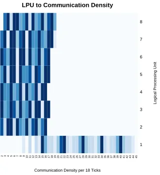
3.8
Example of Communication Density graph for the Work-Stealing scheduler
on a Core i7 running the
P Ring
(defined in section 3.3.2) application. . . .
29
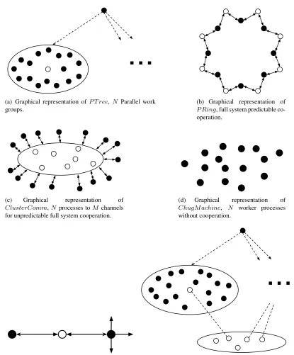
3.9
Simulated behavior examples and test primitives. . . .
33
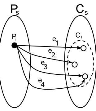
3.10 Bipartite Graph of Processes (
P s
) to Channels (
Cs
). . . .
38
4.1
Our implementation for a map-reduce style fork-branch, and its subsequent
standardized usage. . . .
41
4.2
Parallel Fibonacci implementation and a potential channel graph. . . .
42
4.3
The tick-disparity for over nearly
900
tests. . . .
44
4.4
A naive but ineffectual
ClusterComm
(
N,M
)
implementation. . . .
66
1.1
ChugMachine application, generates
N
processes to just compute. . . .
71
1.2
UserInput application, utilized in the Interactivity composure, it artificially
hangs without anything to do for a random period of time so as to simulate
an interactive process. . . .
72
1.4
PRing application, simulates full-system cooperativity, where
N
processes
pass a token around a ring network.
. . . .
74
1.5
PTree application, utilizes composure of ClusterComm to simulate
partial-system cooperativity as a set of work-groups. . . .
75
1.6
Interactivity Application, utilizes a composure of UserInput.els and
Chug-Machine.els to test a scheduler’s ability to handle interactivity. . . .
76
1.7
JumpShip application, similar to PTree and ClusterComm, except posses to
Chapter 1
Introduction
Runtime systems can be broken up into several distinct parts: the garbage collector,
dynamic type-checker, resource allocator,
etc.
One subsystem of a language’s runtime is the
task scheduler
. The scheduler is responsible for ordering task evaluation and the distribution
of these tasks across the available processing units.
Tasks
1
are typically spawned when there is a chance for parallelism, either
ex-plicitly through
spawn
or
fork
commands or implicitly through calls to parallel built-in
functions like
pmap
. In either case it is assumed that the role of a task is to perform some
action concurrent to the parent task because it would be quicker if given the chance to be
parallel. It is up to the scheduler of these tasks to try and optimize for where there is
op-portunity for parallelism. However, it’s not as simple as evenly distributing the tasks over
the set of processing units. Sometimes, these tasks need particular resources which other
tasks are currently using, or perhaps some tasks are waiting for user input and don’t have
anything to do. Still worse, some tasks may be trying to work together to complete an
objective, and rely on dynamic dependencies that change over time.
Message passing is a common alternative to, and sometimes abstraction of, shared
memory. Some implementations of message passing are akin to emailing a colleague a
question. You operate asynchronously, and your colleague can check her mailbox and then
respond at her leisure. Meanwhile you are free to wait until she gets back to you, or ask
1
someone else in the mean time. Other implementations require you to wait on your
col-league’s reply before continuing.
While message passing is a good method for inter-process communication, it is
also a nice mechanism for catching when two processes are working together. For example,
consider a purely functional
pmap
, where all workers are given subsections of the list. Each
worker thread will have no need to access another’s subsection and thus no messages will
need to be passed. However, what happens when the function being mapped on a particular
subsection uses several processes? Each may access a shared resource via message passing.
We would observe a close coupling of processes in this case. This highlights the granularity
of process coupling, in that the
pmap
workers exhibit coarse-grained parallelism, which
allows the scheduler greater flexibility to run them in parallel. The opposite is true for the
processes which show close coupling, like the mapped function. We define this granularity
of process coupling as
Process Cooperativity
.
There are many mechanisms that scheduling systems can use to improve workload
across all processing units. Some of these mechanisms use what is called a
feedback
sys-tem
. Namely, they observe the running behavior of the application as a whole, (
i.e.
collect
metrics
), and modify themselves to improve operation.
Process Cooperativity
is an interesting metric by which to grade a system. In
bio-chemistry the term cooperativity is defined as an increase or decrease in the rate of
inter-action between a reactant and a protein as the reactant concentration increases. We can
translate this into an information theoretic definition:
Definition 1.
The degree of cooperativity of a
process
is the increase or decrease in its rate
of interaction with an inter-process communication method, and subsequently, the degree
of cooperativity of the
system
is the rate of interaction between the sets of processes and
Thus, when a process attempts to pass a message to another we know it’s trying
to cooperate on some level. When this frequency of interaction is high, it may indicate
a tight coupling of processes or fine-grained parallelism. If it is low, this could indicate
coarse-grained parallelism. In either event, a scheduler able to recognize these clusters of
cooperative and non-cooperative processes should have an edge over those that don’t.
Chapter 2 will look first at the background of classical scheduling systems as well
as the recent feedback-enabled approaches. Then, we will also examine the types of
mes-sage passing implementations and how these effect scheduling decisions, now that we are
looking at process cooperativity. Chapter 3 introduces our work on a language and compiler,
built to easily simulate system cooperativity and visualize the effects of scheduling
mecha-nisms on these systems. We also discuss a few example mechanics which take advantage of
cooperativity. Some example applications which demonstrate different degrees of
coopera-tivity and phase changes are also explained. In Chapter 4 we run our cooperacoopera-tivity-enabled
schedulers along with a few common non-feedback-enabled schedulers on the example
ap-plications and discuss the results. Finally, in Chapter 5 we give some concluding remarks
Chapter 2
Background
2.1
Message-Passing
In concurrent systems, there are a number of methods for inter-process
communica-tion. Arguably though, one of the more popular abstractions is the idea of message passing.
This is especially true in functional languages as the language assumes shared-nothing by
default. Also, just as compilers can optimize using language constraints, so can a runtime
using the language implementation. We will therefore examine possible message passing
designs and how their implementation might effect our schedulers.
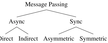
Message Passing
Sync
Symmetric
Asymmetric
Async
[image:15.612.224.412.386.461.2]Indirect
Direct
Figure 2.1: A High-Level Message-Passing Taxonomy
Message passing in general can be broken down into two types based on the
lan-guage’s implementation; asynchronous or synchronous. Asynchronous message passing
is like our example of emailing a coworker. The two actors in the scenario can perform
their communication operations at different times and do not rely on the other’s
comple-tion. Granted, a receive will not complete successfully until after a send has finished.
Synchronous message passing however, requires that both actors block on their respective
In
direct
asynchronous message passing, a process can send the message directly to
another process like in our example of emailing a coworker; these implementations are aptly
named mailbox message passing. An alternative implementation may send the message
indirectly
via a rendezvous point, like a socket.
To send a message in either case requires pushing/copying the message into a
shared or global memory space for another process to access (possibly) at a later time. This
push/copy can be done in a lock free manner with some lower level atomic data structures
such as a double-ended queue. But in either a locked or lock-free manner, the process
per-forming the send still forces a block somewhere along in the operation, to push the message
into shared storage. While asynchronous operations free user-code to continue, its
imple-mentation now requires the additional capabilities to both store and resend a message at a
later time. So at some point, a process will need to synchronize with a block of memory to
enforce exclusive access. If the implementation were to ignore this, contention could occur
between two internal processes attempting communication operations with the same block;
either overwriting or corrupting what was already there.
In terms of scheduling, a language with asynchronous message passing will not
hint much in regard to whether progress is being made. If a consumer process requires a
value before continuing and therefore is repeatedly trying to receive from the channel, the
schedule for the system would be better served by coming back to that process at a later time
rather than repeatedly looping. However, asynchronous can benefit from process placement
so as to take advantage of possible gains in cache affinity [1].
For example, the effects of the cache on direct message passing (
e.g.
a process
mailbox) can be substantial if two processes on different cores share a location to store and
therefore check for content. This shared location, if accessed from two cores will need to
be updated in possibly multiple locations and validated for consistency at the cache level.
switching and cache-line validation. In indirect message passing the task can be even worse
as it’s common that more than two processes may need access to the same space. Note,
however, that recognizing cache effects can also lead to gains in synchronous message
passing.
In synchronous message passing, a process must meet another at a provided
ren-dezvous point but can either be symmetrical or asymmetrical. Note that the renren-dezvous
point is not a requirement in the sense that direct synchronous messaging isn’t possible.
Instead we think of a rendezvous point in synchronous communication to be time bound
rather than location bound (
i.e.
two processes are blocked until communication occurs, the
implementation of this passing is irrelevant to this classification).
Asymmetrical message passing is synonymous with Milner’s Calculus of
Com-municating Systems [2] or standard
Π
-Calculus [3], in that you have a sender, and then a
receiver which will both block on their respective functions around an anonymous
chan-nel until the pass has been completed. This differs from symmetrical message passing,
where the only operation on the channel is a blocking function which swaps values with the
process at the other end.
It’s worth noting that asynchronous message-passing can be simulated using
syn-chronous channels with a secondary buffer process. But by simulating it in this fashion we,
as the scheduler, elevate the problem of cache locality to a problem of process locality. The
same methods suggested to alleviate some of the lost efficiency due to cache locality [4,
5] are the same techniques which could be simulated for process locality; namely process
batching and process affinity.
Note also, it is possible to simulate symmetrical message passing on asymmetrical
message channels, but in terms of scheduling of synchronizing processes, order is now
which complicates the channel implementation. Namely, the internal queuing of senders or
receivers may not percolate hints up to the scheduler regarding their queue position.
For the alternative, symmetrical message passing or swap channels, the order is
directly handled by the scheduling of the system (
i.e.
the order at which the scheduler
evaluate the
swap
command can be directly governed). And it is for this purpose along
with simplifying our core language we have chosen to base our semantics on symmetric
synchronous message-passing.
2.2
Classic Runtime Scheduling
Operating Systems research has long been the leading front for scheduling topics.
However, most of the early concern in scheduling was devoted to job scheduling over a
group/shared system. As such, their concerns were largely devoted to fairness and job
priority. They frequently had
a priori
knowledge regarding their jobs which gave them an
opportunity to decide on a complete schedule beforehand.
Instead, the systems for which we can schedule must be defined differently. A
runtime scheduler may only have access to the processes which it observes, and can only
speculate about their future based on their current state and any recorded historical
infor-mation.
A scheduler’s operations can be defined in a discrete set of time-steps where,
through our definition, must perform three operations for each step. First, it takes the set of
processes and chooses one. This selection operation can be as simple as popping from the
top of a queue but is defined by the private state of the scheduler. As such, it can change
with time or be based on the recorded historical state of the processes.
Next, it will perform some reduction action on the chosen process; taking into
modification of the scheduler’s private-state (
i.e.
due to additional historical records), the
global channel state (
i.e.
with the creation of a new message passing channel), or possibly
the generation of another process, in the case of a process spawn.
Finally, the scheduler will update the process set with the reduced process (and any
generated processes). This update may also modify the private state of the scheduler, which
could store statistics like a process’s historical information. This state update can influence
its selection for the next step, like choosing the oldest process, or the one last seen,
etc.
We base our Scheduler API (section 3.2.3) on this idea of a constant tick function,
which maps the state of the scheduler’s world to the world after one time-step. Multiple
schedulers can then be run in parallel using the same step semantics, except now the total
process queue must be shared or partitioned depending on the scheduler’s unique
imple-mentation.
However, outside of this unique formalism, there is a large set of classical
method-ologies for these operations (
e.g.
selection, reduction, process set update). We now turn to
a description of some of these to lay a basis for our later design discussion.
One popular selection operation is the First-Come, First-Serve method, which means
ordering the processes in a queue and running them continuously as they spawn and
enqueu-ing them only as they block. However, if a particular process is computationally intensive,
processes involved with user-interaction for example would need to wait. This results in an
obvious lag or hang in the system as the interactivity of the system stalls to finish
computa-tion.
To solve this problem a scheduler can
preempt
a process after a certain amount of
time has passed. This time slice is also called a time interval or a
quantum
and has quite
a literature involved with its selection [6, 7, 8]. Too short, doesn’t allow a process enough
computation. Too long and the preemptive-scheduler effectively becomes non-preemptive
as all computation-bound processes hog the CPU from the interactive ones.
We translate this idea of a quantum to the simple step formalism by allowing the
scheduler to keep track of a reduction count. This reduction count influences where the
update operation places the process at the end of the step. If it has reached some max
reduction count, then it could be enqueued at the end of the process set. Alternatively it can
be placed at the beginning to be selected again until after preemption.
This strategy, to enqueue at the end upon preemption, is known as
round-robin
scheduling
. It is a common choice not necessarily due to its simplicity, but its fairness.
Each process in the queue is guaranteed an equal amount of time on the CPU and starvation
of processes can therefore never happen. However, this isn’t always the case as it depends
on how process spawning is implemented. For example, if the newly spawned process was
placed at the front of the queue or preempts the currently running process, a fork-bomb like
process could hog the CPU and effectively shut out all other processes. Spawning to the end
of the queue is the only effective way to avoid these scenarios with round-robin scheduling.
This, however, has all been using the assumption of a single process queue. While
it is possible to implement a single global queue for all
P
processors, we will eventually get
into an issue of contention where all the processors are attempting to take or add a process
to the queue while another one is. However, in the event of multiple process queues there
needs to be a mechanism in place for dispersing the processes across them all in an even or
fair way.
There are two mechanisms for this, namely,
work-sharing
and
work-stealing
. In
work-sharing, the processor with more than enough work to do, will delegate any new
pro-cesses to another (either randomly or by some heuristic). In work-stealing, it’s the scheduler
with the empty or small process queue that contacts another scheduler (either randomly or
the victim processor can be working on a process while another processor steals from it.
In turn, the cost of performing the process transfer is potentially masked by the parallelism
gained. In the case of work-sharing there is always an additional overhead incurred on top
of process execution as the overloaded processor must wait until the delegated process is
transferred.
This is why most schedulers which support multiple processing units utilize some
work-stealing implementation. Of the implementations, there are two which we would like
to highlight as they are provided by the ErLam toolkit: Shared-Queues and
Interrupting-Steal. The Shared-Queues work-stealing scheduler allows other processes to directly access
an end of their local process queue. This means, while a processor is potentially popping
from one end of the queue, another could be stealing from the other end (assuming a
lock-free doubly-ended queue like structure).
The alternative, Interrupting-Steal, has gone by several names like Work-Requesting,
and Thief Processes. It’s mechanism is to send a fake or dummy process to one or more
other schedulers so when they run them they steal a process and send it back to its
par-ent process. This reduces the overhead involved in synchronizing on the victim’s process
queue, but will instead stall it during the steal.
2.3
A Note on Control Theory
There has never been a scheduler which works optimally in all cases. Since for
any scheduler, a program can be feasibly designed for which the scheduler produces a
sub-optimal schedule. Instead, focus has been the most fruitful when pursuing the optimization
of various measurements using some particular objective function [9] to tune for particular
edge cases. As such, scheduling based on such feedback metrics is not a new practice [10].
There is a big distinction though, which can be made between the effects of control
Figure 2.2: A classical feedback loop representation [11].
in the adaptation of the controller in the generic feedback loop (figure 2.2).
The classic feedback loop starts by reading the current state of the system and
applying some operation to it (via the controller). The operation in some way affects the
system which can be observed by measuring particular metrics. These measurements can
be fed back to the controller along with details about the system’s output. If the controller
wishes to modify the system further via the same or an opposite operation, it may do so.
The canonical example is that of an automobile’s cruise control. The controller can correct
the speed of the vehicle by applying or releasing the throttle based on readings of the current
speed so as to maintain a desired speed.
In typical physical feedback loops there are two scenarios which need to be avoided:
resonance and rapid compensation. Resonance in physical systems is when a spike in the
amplitude of a system’s oscillation can cause it to fail at a particular frequency. It can be
seen that most controller models will attempt to damp the adjustments to reduce oscillation
which could cause resonance or sharp spikes in behavior based on its output. This is due
to the limitations of the physical space in which they are having to work. But frequent or
extreme damping or can stress physical systems to the point of failure as well.
However, in runtime scheduling systems we would very much like to do the
oppo-site. We would prefer tight oscillations or consistent behavior of our runtime so as to achieve
minimal overhead from our modifications. We can also compensate, to reach our reference
As such these feedback systems are closely coupled with the design of the scheduling
al-gorithm, rather than being an interchangeable sensor, and controller modules. As such we
make an effort to trace the feedback optimizations during our evaluation and explanation of
the scheduler designs.
2.4
Feedback-Enabled Scheduling
Operating systems have also had motivation for designing intelligent
feedback-enabled schedulers. As systems move away from perfect knowledge about the jobs it will
be running, scheduling has needed to make guesses about the length of time jobs will need
to run. A well-known example to this effect is called the Multi-Level Feedback Queue
(MLFQ) scheduler, first described by Corbat´o
et al.
[12, 13].
The scheduler maintains
N
separate process queues, for
N
priority levels. All new
processes would be spawned to the highest priority and would be subsequently demoted if
they ended up running their whole designated quantum. However, a process may
inadver-tently game the system by running just up to the quantum before yielding. To fix this, after
some time,
S
, the MLFQ is reset and all processes are boosted to the highest priority. This
helps with adapting to new system behavior which may arise as well as coping with process
starvation.
The goal of the MLFQ model is two-fold: to prefer interactive processes and to
subsequently reduce the strain of computation bound processes on the overall system. This
allows the system to prune the short-running processes out quickly and also maintain an
adequate level of interactivity. A MLFQ implementer would also be able to heuristically set
the quantum,
N
, and
S
based on the needs of the system as it’s running, so as to introduce
a second layer of feedback. For example, one could observe how much of a particular time
period each priority queue is using. If a lower priority queue is being starved, it could
The MLFQ idea in general is highly malleable and can be adapted to a number of
situations. As such it transferred well into the level of runtime systems quite well.
Concur-rent ML (CML), uses this idea of a MLFQ to improve application interactivity.
CML is an extension to SML which adds the
spawn
function, and channel
oper-ations, among other things (such as synchronous events) [15]. CML’s scheduler defines a
MLFQ where
N
= 2
and uses a single promotion algorithm instead of a reset. However,
there is a key difference: CML uses process tagging to mark whether a process has
com-municated in its last time quantum.
As all newly spawned processes are appended to the primary queue, CML tells
the difference between these newcomers and the short-running processes by tagging any
process which makes a communication, or demoting it if not. A promotion can only happen
if a previously marked process gets a demotion. However, the demotion process of a marked
process is just a mark removal. Thus, the primary queue is essentially two queues in one.
CML’s dual-queue system has the effect of reacting to new processes by testing
them for longevity. It then makes an assumption about their behavior immediately, but a
process can change the scheduler’s first impression of them through consistent behavior
to the contrary. A marked communication-bound process will, if it continues to use its
entire quantum, eventually be demoted. A computation-bound process can eventually be
promoted and marked as a communication-bound if it continues to communicate. Thus the
system eventually adapts its behavior to the new phase of the process.
However, recently an alternative mechanism has been utilized to adapt to system
behavior, that of process batching. The occam-
π
language, and specifically the Kent
Re-targetable occam Compiler (KRoC), allows processes which frequently communicate to be
batched and processed together [16]. This has two side effects: cache-affinity, and informed
The goal of the KRoC scheduler is primarily to take advantage of cache-locality
when scheduling processes. It does so by reducing the chances for cache-misses by
group-ing processes which have a higher likelihood to communicate. The concept begroup-ing, if two
processes communicate, the data which is being shared will be in cache unless too many
context-switches forces it out, thus place them close together in the queue. As a side effect
of this, instead of stealing single processes, the KRoC schedulers will steal batches from
each-other. This results in a quicker equilibrium in work-load saturation than stealing single
processes.
Process migration between batches is done in two ways: 1. A channel synchronizes
and causes the process to be de-scheduled from one scheduler and sent to the one which
unblocks it. 2. A batch is split when more than one process in a batch is active, by popping
the head of the batch into a new one. We explain this de-scheduling method in greater detail
in Section 3.2.2, as we’ve implemented this mechanism for testing purposes. However, the
mechanism absorbs a blocking process into the channel it’s blocked on until another process
unblocks it. At that time, the scheduler which unblocked it, now becomes its owner.
Occam-π
uses this mechanism as a method to build up batches of cooperating processes.
Ritson
et al.
mention however, that without a method to break up the batches, the
system will eventually become one large batch. Therefore, whenever a new process joins
a batch, the batch is allowed to split if there are more than one currently active processes
within it (
e.g.
non-blocked or waiting processes). Thus, if a parent spawns a large number
of processes (
i.e.
passed the batch size limit), the parent can start a new batch, while the
batch of children can be stolen.
While KRoC’s primary goal was cache-affinity, and CML’s was optimizing
interac-tivity, their feedback systems enabled a more efficient schedule than would have otherwise
been possible with a classical scheduler focused entirely on work-saturation. We now
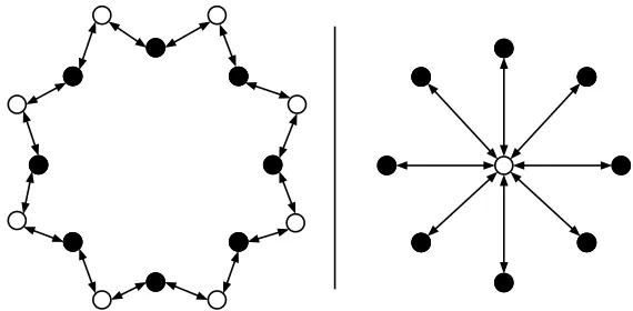
Figure 2.3: Two subcomponents formed by process cooperativity. Black dots represent
processes, and the white dots represent a channel.
algorithms presented later, were able to benefit from.
2.4.1
Cooperativity as a Metric
Process Cooperativity stands out as a critical feedback metric in process-oriented
programming. In fact the KRoC scheduler showed this through their performance gains.
They showed that when a scheduler can recognize when two or more processes form a
sub-component, treating them that way improves cache utilization, reduces context switching
time, and makes for smarter work-stealing. From this, we can take that recognizing
coop-erativity gives a good mechanism for determining a potential for fine-grained parallelism.
However, we would like to revisit the concern Ritson
et al.
expressed regarding
when a component becomes too large. They introduced the mechanism of splitting batches
based on an arbitrary max size of a batch, without regard to the substructure of the
compo-nent expressed by the processes cooperation.
To illustrate this problem, figure 2.3 visualizes two possible components which may
occur naturally. On the left we get a ring like structure, where the dependency of one process
a token ring network. On the right we have a cluster of processes, all communicating with
a random other on the same channel. We can envision this as an abstraction over a single
shared resource.
Both the ring and cluster subcomponents would gradually become grouped into a
KRoC batch. This is optimal for the ring component, no matter how large the ring may
be. There is nothing to be gained from splitting it into multiple batches, and by doing
so, we may actually hinder it. However, the cluster component may improve if given the
chance for more parallelism, this would depend entirely on the
longevity
of the processes
(
i.e.
the extent the process is computation-bound). KRoC attempts to account for this by
recognizing if there are multiple active processes in a batch, and splitting an arbitrary one
into a new batch (which ever happens to be at the head of the process queue).
While this may not be avoidable based on observing structure alone, we may now
run into an issue. Suppose all processes are active, but run for a length of time under their
designated time quantum. At every preemption, when the size of the batch forces a split,
we will create a singleton batch which must be reabsorbed after a single run. Ignoring the
overhead, fairness properties also start to percolate. Namely, the processes within the batch
after being trimmed will get preferential treatment to the processes in the singleton batches.
This is exacerbated in the case of a single processor, as all singleton batches would need to
wait for the large batch to run. Inevitably, the worst-case scenario for KRoC is below that
of the work-stealing scheduler.
From this we can take that the longevity of a process can affect its cooperativity.
In fact, we can look back at definition 1, and its application to a single process. A process’
degree of cooperativity
can be defined as its
frequency
of interaction with a set of channels.
Thus, a cooperativity-conscious scheduler should also want to consider both the longevity
of a process, and which channels it communicates with. This would give a much more
Chapter 3
Methodology
3.1
Overview
To examine the effects of cooperativity-conscious schedulers we needed to have a
method for comparing several scheduler implementations without needing to modify the
underlying implementation of processes, channels, or application source code. It would be
also beneficial if our solution were able to visualize these differences similar to Haskell’s
ThreadScope [17].
Our solution,
ErLam
, is a compiler for an experimental version of Lambda
Calcu-lus with Swap Channels and a runtime system which allows for swappable scheduler
mech-anisms and an optional logging system which can be fed into a custom report generator. We
break up our solution description into three parts; Section 3.2 will discuss our language
syn-tax and semantics. It will also demonstrate our Runtime Scheduler API by breaking down
the CML Interactivity scheduler. Section 3.3 will go more into depth about our testing
en-vironment which involves our logging system, the report generator, and the set of example
applications we used to represent different cooperativity levels. Finally, Section 3.4 will go
over our example schedulers we wrote which demonstrate cooperative-conscious behavior.
These will be the schedulers we provide our results against.
3.2
ErLam
The ErLam toolkit is itself broken down into three parts, the language and its
<Expression> ::= <Variable>
|
<Integer>
|
‘
newchan
’
|
‘
(
’ <Expression> ‘
)
’
|
<Expression> <Expression>
|
‘
if
’ <Expression> <Expression> <Expression>
|
‘
swap
’ <Expression> <Expression>
|
‘
spawn
’ <Expression>
[image:29.612.153.475.118.214.2]|
‘
fun
’ <Variable> ‘
.
’ <Expression>
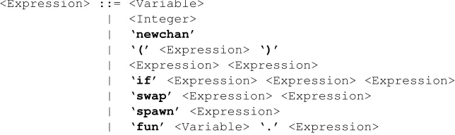
Figure 3.1: The ErLam language grammar, without syntax sugar or types.
its basic semantics, as the finer-details are reliant on the exact selected scheduling solution
as well as the chosen swap-channel implementation. We will then examine the possible
channel implementations and how they affect the given semantics. Next, we will discuss
the Scheduler API using an example scheduler implementation. We conclude this chapter
with a summary of each of the classic schedulers that are included in the ErLam toolkit.
3.2.1
The ErLam Language
The ErLam Language is based on Lambda Calculus, with first-class single variable
functions, but deviates somewhat in that it provides other first-class entities. It deviates
from Church representation to provide Integers, however, this is purely for ease of use. It
also provides a symmetric synchronous channel type for inter-process communication.
Figure 3.1 expresses ErLam in its simplified BN-Form. The semantics for the
lan-guage is fairly straight forward. All expressions reduce to one of the terminal types: Integer,
Channel, or Function. To spawn, for instance, if any terminal is passed other than a
func-tion, it returns a
0
(
e.g.
false). When a function is passed, it is applied with
nil
to initialize
the internal expression in another ErLam process, and evaluates to
1
(
e.g.
true) in the parent
process.
ErLam also makes a number of ease-of-use decisions like providing a default branch
oper-let
x
=
e
1
in
e
2
⇒
((
fun
x.e
2
)
e
1
)
fun
x,y,z
.
e
⇒
fun
x
.
(
fun
y
.
(
fun
z
.
e
))
Figure 3.2: Syntactic sugar parse transformations.
ations, type checking, and standard functional behaviors (
e.g.
combinators,
etc.
). However,
these built-ins will be largely ignored in this document but explained when necessary. The
branching operator works like C in that zero is interpreted as false and non-zero is true.
ErLam also extends this base grammar with some useful syntactic sugar (see
fig-ure 3.2 for syntactic transformations) such as SML style
let
expressions and multi-variable
function definitions (which are curried from left to right). We will use the syntactic sugar
throughout this document to make our source easier to review.
Also, note that the semantics of
swap
is to block until a successful swap. However,
the implementation of the channel synchronization is free to change as long as it adheres.
We take advantage of this to provide multiple channel implementations which will
high-light distinct scheduling differences. We demonstrate this, along with an example ErLam
application in the following section.
3.2.2
Channel Implementations
ErLam provides a selection of channel implementations to allow for
interchange-able scheduler comparisons with different synchronization methods. We chose two channel
implementations the
Blocking
Swap, and the
Absorbing
Swap as they highlight key
differ-ences for the runtime. We will now look at an example application and its execution using
both methods for comparison.
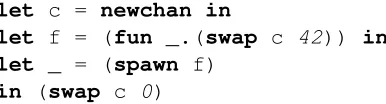
Figure 3.3 gives an example ErLam application. It first creates a new channel for
let
c =
newchan in
let
f = (
fun
_.(
swap
c
42
))
in
let
_ = (
spawn
f)
[image:31.612.219.412.116.168.2]in
(
swap
c
0
)
Figure 3.3: A simple ErLam application which swaps on a channel before returning.
is to swap on the channel the number
42
and quit. Finally, it swaps on the channel the
number
0
and returns the result of the whole evaluation, which in this case will be the value
passed from the other end of the swap,
42
.
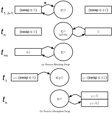
As ErLam is innately concurrent, we do not know which process will ask to swap
first. It may even be possible that
0
asks to swap several times before
42
even tries. In
fact, the
Blocking
channel allows this behavior of multiple swap attempts. We can see an
illustration of this in figure 3.4(a). The first row shows the arbitrary time-slice
t
1
where
the process swapping
0
,
p
0
, first contacts the channel with its value. The process may be
scheduled again, repeatedly, to check the channel up to some arbitrary time-slice
t
n
−
1
. At
t
n
however, the process swapping
42
requests a swap and immediately gets a value back
and logs that the process which it swapped with can get its value when it returns. Thus on
the third line, for any arbitrary time-slice in the future
t
>n
, the process
p
0
can ask for a
swap and get the value
p
1
stored.
Note the illustration makes no explicit mention of the scheduler or its functionality.
It may be the case that the two processes are on different processing units and are in different
process queues. Or it may be the case that they both exist in the same queue and upon a
block, the scheduler chooses the next one, which will immediately unblock the channel.
The
Blocking
channel effectively simulates a common spin-lock over a shared piece
of memory. These channels represent a worst-case, albeit common, application
implemen-tation for concurrent software. Even so, they do allow for some hints to the scheduler,
Er-(a) Process Blocking Swap
[image:32.612.124.514.173.566.2](b) Process Absorption Swap
Figure 3.4: Channel operation over time. Note arbitrary time-slice
t
1
is when the first swap
-
callback
layout(
erlang
:cpu_topology(), scheduler_opts() ) ->
scheduler_layout().
-
callback
init( scheduler_opts() ) ->
{ok, scheduler_state()} |
{error, log_msg()}
|
{warn, log_msg(), scheduler_state()}.
-
callback
cleanup( scheduler_state() ) ->
ok | {error, log_msg()} | {warn, log_msg()}.
-
callback
tick( scheduler_status(), scheduler_state() ) ->
{ok, scheduler_status(), scheduler_state()} |
{return, term()} | {stop, scheduler_state()}.
-
callback
spawn_process( erlam_process(), scheduler_state() ) ->
{ok, scheduler_state()} | {error, log_msg()}.
Figure 3.5: The ErLam Scheduler API
Lam toolkit though, such as a push-notifying semaphore, however we provide a simpler and
functionally more common alternative: the process absorption channel.
In the
Absorption
channel (figure 3.4(b)), the first process to get to the channel will
get absorbed by it. The scheduler which evaluated the swap will be out a process, and but
the scheduler which unblocks the channel by arriving second will get back two processes
(the one performing the swap, and the absorbed one). In terms of scheduling efficiency this
type of message passing channel has provided enormous improvements for runtimes which
do not wish to introduce channel inspection into their scheduler.
3.2.3
The Scheduler API
ErLam was written in Erlang, and as such, can take advantage of Erlang’s
call-back behavior specifications. An
erlam scheduler
behavior was defined which requires a
minimum of
5
callback functions (figure 3.5).
Non-uniform Memory Access (NUMA) layout of the system that the application is running on,
along with any parameters the user specified at runtime. The result of this function is to be
the scheduler layout.
For example, let’s assume we are running our application on a Intel Core i7 which
has 4 logical cores which support hyper-threading. The
layout/2
function will be given the
following structure:
[{processor,[{core,[{thread,{logical,0}},{thread,{logical,1}}]},
{core,[{thread,{logical,2}},{thread,{logical,3}}]},
{core,[{thread,{logical,4}},{thread,{logical,5}}]},
{core,[{thread,{logical,6}},{thread,{logical,7}}]}]}].
This indicates to the scheduler implementation that it, at max, can spawn
8
instances of
itself which would be bound to each logical processing unit (LPU). Although we could
of course have a scheduler which acts differently based on the architecture. However, the
schedulers we have limited ourselves to are either single or fully multi-core (
i.e.
uses all
available LPUs).
To spin up an instance of the scheduler on the particular core, the
init/1
function
is called which should return the scheduler’s state. As Erlang is a functional language, we
use this state object as a means to maintain some global state for each scheduler process by
threading it through all subsequent callback calls. Upon shutdown, the opposite function
cleanup/1
is called.
The last two functions are the most interesting as they pertain to the core of what
each new scheduler provides, namely how to evaluate the world in a given time-slice (
tick/2
)
and how a new process should be handled (
spawn process/2
). An explanation of these
spawn_process( Process, State ) ->
enqueueAndSwitchCurThread( Process, State ).
enqueueAndSwitchCurThread( Process, #state{curThread=T}=State ) ->
case
T
of
nil ->
setCurThread( Process, State );
_
->
% New process takes over
{ok, NewState} = enqueue1( T, State ),
setCurThread( Process, NewState )
end
.
Figure 3.6: CML Process Spawning.
3.2.4
Example Usage: The CML Scheduler
CML’s scheduler utilizes a dual-queue structure rather than a simple
unary-process-queue. The scheduler attempts to differentiate between
communication
and
computation
-bound processes so as to reduce the effects of highly computationally intensive processes
from choking the system. The scheduling system thus improves on application interactivity
by demoting
computation
-bound processes to the secondary queue (which isn’t accessed
until another process is demoted).
Spawning a process in the CML scheduler (figure 3.6) does not go onto the primary
queue, instead we enqueue the current process and start evaluating the new process
1
. This
is a fairly simplistic example, but it shows how one would go about updating the state
between ticks. Note also, that the
spawn process/2
call happens on the same scheduler
instance which evaluated the
spawn
. While this is not of consequence for this scheduler,
a multi-core scheduler could be confident in appending a new process to its local queue
without interfering with another LPU’s scheduler.
1
tick( _Status, #state{ curReduct=0 }=State ) ->
{ok, NState} =
pick_next( State ),
reduce( NState );
tick( _Status, State ) -> reduce( State ).
pick_next( State ) ->
{ok, NewState} = preempt( State ),
% Place cur thread onto queue
{ok, Top, Next} = dequeue1( NewState ),
% Pop next off
setCurThread( Top, Next ).
% Set as cur and return state
Figure 3.7: CML Process evaluation.
In the original CML scheduler, it defined a quantum which it would let the current
process run for, it would preempt it if it attempted to run for longer. The ErLam runtime
avoids the use of time based quantum as logging and other factors directly affect the
useful-ness of this. Instead it uses a ‘tick’, which emulates one step forward in the execution of the
application. Thus to simulate a quantum we instead keep track of the number of reductions
performed on the current process and decrement the counter until we reach
0
.
The
tick/2
function (figure 3.7) performs one of two things based on what the state
of the system is. If the current reduction count is
0
, then we can pick a new process from
the queue, otherwise we can perform a reduction.
Note for our scheduler simulation we ignore the first parameter to the
tick/2
func-tion for either case. The first parameter was the status of the scheduler returned from the
previous tick (
e.g.
running, waiting,
etc.
). This would be useful if the CML scheduler
uti-lized work-stealing to get work to do from other LPUs when in
waiting
mode.
3.2.5
Provided Schedulers
Along with the Single-Threaded Dual-Queue CML scheduler
(STDQ)
, ErLam comes
with several basic scheduling mechanics. We utilize these as bases cases on which to
•
The Multi-Threaded Round-Robin Global-Queue Scheduler
(MTRRGQ)
This scheduler uses a single global process queue which all schedulers share and
attempt to work from. There is no rearrangement of order, and all threads will
round-robin the queue (performing a set number of reductions per process before enqueuing
and popping the top one).
– The Single-Threaded Round-Robin Scheduler
(STRR)
This scheduler is a special case where
P
= 1
. We provide a simplified
imple-mentation which removes all synchronization of the previous scheduler. This
will be our simplest scheduler test case, and will be compared against
STDQ
.
•
The Multi-Threaded Round-Robin Work-Stealing Scheduler
(MTRRWS)
An improvement on the previous scheduler. Instead of a global process queue, each
scheduler maintains their own. A waiting scheduler will randomly sleep-and-steal
until it finds a process to work on from another scheduler. The provided
implemen-tation gives two example stealing mechanisms:
– Shared-Queue
(MTRRWS-SQ)
Stealing a process involves performing an atomic dequeue from the bottom
(rather than the top) of another scheduler’s process queue. This will only block
the other scheduler from performing a dequeue for a very short window of time,
but the other scheduler must compensate for this concurrent access by
synchro-nizing on its usage as well, despite the relative infrequency of steals.
– Interrupting-Steal
(MTRRWS-IS)
Simulates sending a thief-process over to another scheduler. When the victim
scheduler preempts or yields their current process and selects the next one from
the queue, they can instead check for a thief process which may syphon a
a longer period of time, but uses ErLam’s inter-scheduler message-queue rather
than synchronizing on another LPUs process queue. This secondary queue can
be accessed less frequently and at the scheduler’s discretion so the
synchro-nization overhead isn’t incurred upon standard usage (as no other scheduler can
access the local process queue).
ErLam also comes with three cooperativity-conscious schedulers: the
Longevity-Based Batching Scheduler (section 3.4.1), the Channel Pinning Scheduler (section 3.4.2),
and the Bipartite Graph Aided Sorting Scheduler (section 3.4.3). The first two build on the
same shared queue module as provided by
M T RRW S
-
∗
, while the third utilizes its own
implementation.
For any compiled ErLam script, the runtime installs a command line option for
selecting the scheduler used (among several other options). We are able to specify that we
wish to run
pf ib
, for example, with
M T RRGQ
with the following command:
./pfib -s erlam_sched_global_queue
Any new schedulers can be added to the ErLam toolkit without needing to recompile the
scripts as they are dynamically fetched and loaded at runtime.
3.3
Simulation & Visualization
The second primary goal of the ErLam toolkit was the ability to visualize how a
scheduler proceeded to evaluate an ErLam application. We therefore needed a way to log
all events over time, including unique per-scheduler events, such as the size of both the
primary and secondary queues in the CML scheduler. It would also be advantageous to
be as finely grained as possible and leave it up to the visualization mechanism to dial the
We also needed a sample set of application simulations to run our set of schedulers
against. These simulations needed to be minimal to reduce extraneous data but still
demon-strate various levels of cooperativity and phase changes. We would like to also have the
ability to compose test cases together to better create realistic work-sets for the schedulers
to react to.
3.3.1
Runtime Log Reports
Logging in Erlang is a fairly simple matter. We utilize a simplistic data logging
module based on syslog. The output of running an application could look like this:
timestamp,lpu,event,value
...
983847.935268,3,sched_state,running
983847.935333,0,queue_length,59
983847.935677,24,channel_blocked,6102
983847.935683,6,yield,""
983847.936003,4,queue_length,50
983847.936430,3,tick,""
983847.936439,3,reduction,""
...
The time-stamp given is a concatenation of the second and microsecond that the event
happened in. The lpu is the scheduler which caused the event, unless it’s a channel based
event, such as a
channel blocked
event, in which case it’s the channel ID.
Our logging API is fairly simplistic as we only need to capture two types of metrics
from our events: quantity and frequency. With frequency, we want to know the amount of
events which happened in a time range, but with quantity we would like things like length
of the scheduler’s process queue over time or the amount of time spent in the running or
waiting state.
Note time is not consistent per LPU, it may be the case that another OS application
1
2
3
4
5
6
7
8
9
10
11
12
13
14
15
16
17
18
19
20
21
22
23
24
25
26
27
28
29
30
31
32
33
34
35
36
37
38
39
40
41
42
43
44
45
Communication Density per 18 Ticks
1
2
3
4
5
6
7
8
Logical Processing Unit
[image:40.612.236.401.114.295.2]LPU to Communication Density
Figure 3.8: Example of Communication Density graph for the Work-Stealing scheduler on
a Core i7 running the
P Ring
(defined in section 3.3.2) application.
of the LPUs getting far less
“tick”
events. Worse yet, there may be a large gap of time
missing from one scheduler to the next. For our purposes though we would like to compare
the state of the scheduler while it is executing and would be fine with averaging over the
largest gap. These from experimentation have not been found to be very frequent or large
on an otherwise unoccupied processor (see section 4.1.2 for details).
To explain this averaging technique we’ll now discuss the report generation method.
The ErLam toolkit comes with a secondary R script which can be given a generated log file
for processing. This script dynamically loads chart creation scripts based on the types
of events it sees in the log file. The toolkit comes with five charting scripts which should
work for all schedulers: Channel Usage (Communication Density) over time, Channel State
(blocked vs. unblocked) over time, Process Queue Length per LPU over time, Reductions
(Computation Density) over time, and Scheduler State (running vs. waiting) over time.
Communication Density for example (see figure 3.8, creates a heatmap based on
the frequency of
yield
events which occur whenever a process attempts a
swap
. Each cell
time-slice for a given LPU. This time-time-slice is where the averages come into play. R heatmaps
have a maximum of
9
colors, so any range we select must be scaled to
9
. However, the
constant multiplicand is based on the mean amount of time
N
ticks take place across each
LPU. We can obviously tune the accuracy of these averages on a per-LPU basis by
mod-ifying
N
. Anecdotally, this turned out to be advantageous on several occasions when
de-bugging scheduler implementations. As decreasing the number of ticks to average together,
increased the number of samples and thus accuracy.
3.3.2
Cooperativity Testing
As part of the thought experiment, we needed to implement a decent set of test
cases which would give us a good coverage of the range of cooperative behavior in common
applications.
On one hand we have an axis depicting the amount of parallelism possible in an
application. A system which is completely parallel, would be one where all processes
spawned have no dependence on any of the others. For our toolkit, we called this behavior
ChugM achine
N
(figure 3.9(d)) ; where
N
depicts the number of parallel processes. On
the other side of the axis, we would have a system which had absolutely no parallelism
possible. We called this behavior
P Ring
N
(figure 3.9(b)), as it would spawn
N
processes
in a ring formation and pass a token in one direction. Each process has a channel to its left
and right and would synchronize to the right until it receives a token to continue.
P Ring
N
also gives an example of full-system cooperation, except we would
in-stead like some degree of parallelism possible. To experiment with that, we would need
to throttle the degree of cooperativity. This behavior is called
ClusterComm
(
N,M
)
(fig-ure 3.9(c)) as it spawns
N
processes and
M
channels which can be synchronized with by
any process. Note for this system to work with swap channels we limit
M
to be at most
ClusterComm
(
N,M
)
is also an example of full-system cooperation, we also want
to have a possible case for partial-system cooperation. We begin this range of experiments
with a behavior which acts like a bunch of
ClusterComm
(
N,
1)
running in parallel. We
call this special case behavior
P T ree
(
W,N
)
(figure 3.9(a)); where
W
is the number of work
groups to run in parallel. This is the cleanest case of partial-system cooperation. W
![Figure 2.2: A classical feedback loop representation [11].](https://thumb-us.123doks.com/thumbv2/123dok_us/42042.3633/22.612.178.449.119.186/figure-a-classical-feedback-loop-representation.webp)