A numerical formulation and algorithm for limit and shakedown analysis of large-scale elastoplastic structures

A numerical formulation and algorithm for limit and shakedown

analysis of large-scale elastoplastic structures

Heng Peng1, Yinghua Liu1,* and Haofeng Chen2 1

Department of Engineering Mechanics, AML, Tsinghua University, Beijing 100084, People’s Republic of China

2

Department of Mechanical and Aerospace Engineering, University of Strathclyde, Glasgow G1 1XJ, UK

*

Corresponding author: [email protected]

Abstract

In this paper, a novel direct method called the stress compensation method (SCM) is proposed

for limit and shakedown analysis of large-scale elastoplastic structures. Without needing to

solve the specific mathematical programming problem, the SCM is a two-level iterative

procedure based on a sequence of linear elastic finite element solutions where the global

stiffness matrix is decomposed only once. In the inner loop, the static admissible residual

stress field for shakedown analysis is constructed. In the outer loop, a series of decreasing

load multipliers are updated to approach to the shakedown limit multiplier by using an

efficient and robust iteration control technique, where the static shakedown theorem is

adopted. Three numerical examples up to about 140,000 finite element nodes confirm the

applicability and efficiency of this method for two-dimensional and three-dimensional

elastoplastic structures, with detailed discussions on the convergence and the accuracy of the

proposed algorithm.

Keywords Direct method; Shakedown analysis; Stress compensation method; Large-scale;

Elastoplastic structures

1 Introduction

In many fields of technology, such as petrochemical, civil, mechanical and space engineering,

structures are usually subjected to variable repeated loading. The computation of the

difficult task in structural design and integrity assessment. The full step-by-step elastic-plastic

analysis procedure may be used to estimate the long term behavior of a structure, such as

shakedown, alternating plasticity, incremental plasticity or instantaneous collapse, by the

acquired evolution of stresses and strains. Generally, the method is cumbersome and

time-consuming, and needs the exact knowledge of the loading histories that often are

uncertain in practical engineering situations. A better alternative is to perform the limit and

shakedown analysis of structures using the direct methods [1,2], which just need to know the

interval of these applied loads.

Most of the direct methods are based on the lower bound theorem by Melan [3] or the

upper bound theorem by Koiter [4], both of which rest on the assumptions of perfectly plastic

material, small displacements, negligible inertia and negligible creeping effects [5]. Since the

two pioneering works, the subsequent researches have been along two different routes [6].

The first route of these researches is concerned with the extensions of shakedown theorem,

where the material hardening [7-12], geometric nonlinearities [13,14], non-stationary loads

[15,16], creeping effect [17,18] and frictional contact [19] are considered respectively. The

second route of these researches is concerned with the development of efficient and robust

numerical methods [20-30] towards the solution of the shakedown problem, which is also the

major objective of this article.

Based on the lower or upper bound theorem, the limit and shakedown analysis of a

structure is normally transformed into a mathematical programming problem that aims to

minimize or maximize a goal function under excessive independent variables and constraint

conditions. Different optimization approaches like the nonlinear Newton-type iteration

algorithm [21,29,31], the second order cone programming (SQCP) [32,33] or the interior

point method (IPM) [30,34-37] are widely used for solving the programming problem. Instead

of using the standard finite element method, some researchers combine shakedown analysis

with some other computational methods. The articles about the numerical shakedown analysis

based on the boundary element method [38,39], the cell/edge/node-based smoothed element

method (CS-FEM, ES-FEM or NS-FEM) [40-43], the element free method [44,45], the nodal

discretization or the node arrangement will lead to a tremendous mathematical programming

problem due to the significant number of variables and constraints, which may limit the

application of these methods. In order to reduce the scale of the shakedown problem, some

techniques such as the basis reduction technique [9,44,49] or subspace iteration are employed.

Noteworthy, although the numerical methods mentioned above are based on mathematical

programming, there are some other approaches for limit and shakedown analysis in literatures.

A group of elastic modulus adjustment methods [22-24,50-56], including the generalized local

stress strain (GLOSS) r-node method [50], the m(alpha)-method [51], the elastic

compensation method [22,23,52,53], and the linear matching method (LMM) [24,54-56],

were systematically developed. Using more physical arguments, these methods match the

linear behavior to the nonlinear plastic behavior by performing a sequence of linear solutions

with spatially varying moduli. As the origin of these methods, the elastic compensation

method (ECM) [52] was early put to use for calculating limit loads of pressure vessels. Then

Ponter and Carter [22,23] demonstrated an initial implementation of this technique and also

provided a rigorous theoretical proof for the existence of the monotonically reducing upper

bounds. Finally, a more generalized and practical code called the LMM [24,55-58] was

developed to be used for limit, shakedown and ratchet analyses of engineering structures by

making full use of the commercial finite element software ABAQUS. Further, Garcea et al.

[25,26] propsoed an incremental-iterative solution method which has analogies with the Riks

path-following algorithm to plane frames and two-dimensional flat structures. Another direct

method termed as the residual stress decomposition method for shakedown (RSDM-S) was

presented [28]. Based on the cyclic nature of the residual stress in the steady cycle, the

residual stress at every Gauss point is decomposed into Fourier series in time. This method

was used for evaluating the shakedown loads of some simple two-dimensional structures.

As described above, both the traditional mathematical programming and iterative method

with more physical agreements can be used for calculating the limit and shakedown loads. It

is worth noting that many of the proposed methods appear to aim at academic purpose or to

solve some specific simple problems but are not suitable for general engineering applications.

Even through the shakedown analyses of some complex engineering structures using the IPM

solving large-scale shakedown problems and the finite element models reported in literatures

have no more than 100,000 nodes. From the mathematical point of view, the elastic modulus

adjustment method is not completely satisfactory, because it requires a complete elastic finite

element analysis procedure that includes the assemblage of the stiffness matrix and its

decomposition during every iteration [25].

In this work, a novel direct method named as the stress compensation method (SCM) for

limit and shakedown analysis of large-scale engineering structures is proposed. The method

adopts a two-level iterative strategy where a series of decreasing cyclic loading solutions

based on linear elastic finite element analysis are generated. Over the numerical procedure,

only one decomposition of the global stiffness matrix is required, and the residual stresses are

directly calculated in a very small number of load vertices, which largely enhances the

computational efficiency of the proposed algorithm. By using an efficient and robust iteration

control technique, the convergence and the accuracy of the SCM are ensured. The layout of

this paper is as follows: shakedown criterion and basic theorems for shakedown analysis are

introduced in Sect. 2, followed by description of the formulation of the SCM in Sect. 3. Then

the detailed numerical algorithm of the SCM for shakedown analysis is presented in Sect. 4.

Three numerical examples including two-dimensional (2D) and three-dimensional (3D)

large-scale engineering structures are considered to verify the availability of the proposed

procedure, and the results are also compared to the reference solutions as well as calculations

with the LMM and the step-by-step procedure to illustrate the accuracy and the efficiency of

the SCM in Sect. 5. Finally, the discussion and conclusions are presented in Sect. 6.

2 Shakedown criterion and basic theorems

2.1 Static shakedown theorem by Melan

A lower bound evaluation of the load-carrying capability of an elastic-perfectly plastic

structure under cyclic loading can be obtained by performing the shakedown analysis based

on the static shakedown theorem. The classical conditions of shakedown theorem, such as

extensions are in reach. What’s more, the convex yield surface and the normality rule are

assumed so that the material is stable in Drucker’s sense [30].

The statement of the static shakedown theorem is as follows [59]: a structure will shake

down to the variable repeated loading, i.e. its behavior after a number of initial loading cycles

will become purely elastic, if there exists a time-independent distribution of residual stress

field ρ x

 

such that its superposition with the fictitious elastic stress field σ xE

 

,t , results in a safe stress state σ x

 

,t at any point of the structure under any combination of loads

inside the prescribed domain.

 



,





E

   

,



0

f σ x t  f σ x t ρ x   x V，t (1)

Here, f

 

 is the yield function; σ x

 

,t is the actual stress; σ xE

 

,t is the fictitious elastic stress that occurs if the structure responds to the prescribed loads in a purely elastic

manner; ρ x

 

represents a self-equilibrated residual stress field that should satisfy the

equilibrium conditions within the body V and the boundary conditions on the part Γ_t of the surface, i.e.

in on _t

    

ρ 0 V

ρ n 0 Γ (2)

where   denotes the divergence operator; n is the unit outward normal to the boundary

t

Γ .

2.2 Load domain and specified loading path

Structures are often subjected to many types of loads at the same time, and generally, the

loads vary randomly. If a finite number of the external loads obeying their own rules vary in a

domain, the loading history P x

 

,t can be described as the superposition of these external

loads with different loading sets P x_i

  

, ,t i1, ,N



. The each loading set P x_i

 

,t can be decided by time-dependent multiplier _i

 

t and the normalized basis load 0

 

i

P x .

 

 

   

0

1 1

, ,

N N

i i i

i i

t t  t

 









P x P x P x (3)

 

i i t i

 _ _

(4)

Eq. (3) describes a domain Ω of these loads. The load domain Ω is a polyhedron defined

by m vertices _{B B}1_, 2_{, , B}m _{in the space of load parameters. It is worth noting that the load}

domain Ω may not be convex and the detailed descriptions of load domain for complex

load conditions can be seen in Ref. [60]. As shown in Fig. 1(a), a load domain with five load

vertices is taken as an example.

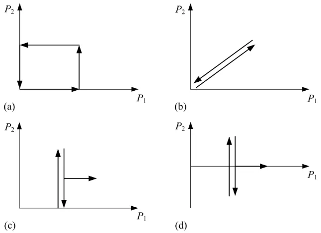
Fig. 1 Load domain and loading path: (a) arbitrary loading path; (b) specified loading path

Although the exact loading history is unknown and the loads may vary in an arbitrary

manner within a domain Ω, the domain Ω is usually known in practical engineering

problems. In order to determine the shakedown behavior of the structure under the load

domain Ω, König [5] proposed a relevant theorem which is stated as follows:

If a given structure shakes down over a certain cyclic loading path which contains all the

m vertices _{B B}1_, 2_{, , B}m _{of the hyper-polyhedral load domain Ω, the structure shakes}

down in an arbitrary loading history defined by Eq. (3).

On the other hand, if the structure does not shake down in a certain cyclic loading path

containing some of the vertices, the direct evidence can be obtained so that the domain Ω is

not a shakedown domain of the structure.

The above statement provides a good strategy to estimate whether or not a given structure

will shake down over any loading path within the domain Ω. We define a specified loading

illustrated in Fig. 1(b). If the structure shakes down under this loading path, then it must shake

down within the load domain defined by all these vertices.

It should be pointed out here that the shakedown analysis will degenerate to the limit

analysis and the plastic limit load can be calculated when the number of the vertices of the

load domain equals to one.

2.3 Steady cyclic stress state

We assume that a body of volume V is subjected to cyclic mechanical loads on a part of the

surface S. The expression of the mechanical loads is as follows:

 

,t 



,tnT



P x P x (5)

where P x

 

,t has the same definition as that in Eq. (3); t is the current time point measured

from the beginning of the cycle; T is the period of the cycle; n1, 2, denotes the number of full cycles; x denotes the coordinates of a material point in the body.

We suppose that the material of a structure is elastic-perfectly plastic and obeys the

Drucker’s postulate. The actual stress σ x

 

,t in the structure is decomposed into two parts:

the fictitious elastic stress part  k_{σ x}E

 

,_{t and the residual stress part ρ x}

 

_{,t , i.e.}

 

 

_{   }

,t k E ,t  ,t

σ x σ x ρ x (6)

where  k is a load multiplier.

The corresponding strain rate can also be decomposed into two parts:

 

 

_{ }

_{ }

,t k E ,t  _r ,t

ε x ε x ε x (7)

where the first term ε xE

 

,t on the right of the equation is the elastic strain rate corresponding to the fictitious elastic stress rate σ xE

 

,t and the second term ε x_r

 

,t on the right of the equation is the residual strain rate. It should be noted that the residual strain

rate ε x_r

 

,t consists of the plastic part ε xp

 

,t and the elastic part ε x_re

 

,t , and ε xe_r

 

,t is required so that the total strain rate ε x

 

,t satisfies the deformation compatibility over the

whole body. Then, Eq. (7) can be written as

 

 

_{ }

_{ }

_{ }

,t  k E ,t  p ,t  er ,t

According to the constitutive law of the elastic-perfectly plastic material with an

associated flow rule, the following equations are obeyed:

 

,

 

,

E E

t   t

σ x D ε x (9)

 

,t   e_r

 

,t

ρ x D ε x (10)

 

,

_{ }

,

p f

t

t

 

 

ε x

σ x (11)

where D is the elastic stiffness matrix; f is the yield function; ε xp

 

,t is the plastic strain rate whose direction is along the outer normal of the yield surface; and  is the plastic

multiplier. Because of the convexity of the yield surface, the following inequality holds

referring to the Drucker’s postulate:



σ σ a



εp0 (12)

where σ is the stress at yield surface associated with the plastic strain rate εp and σa is an admissible stress.

It has been elucidated [59,61,62] that a cyclically loaded elastoplastic structure made up

of material obeying Drucker’s postulate will reach a steady cyclic state, that is, the stresses

and the strain rates will gradually stabilize from cycle to cycle. The stress distribution in the

steady cycle does not depend upon the initial stress state and is unique in those regions where

the plastic strain rates are non-vanishing [59]. However, it should be noted that the

time-independent residual stress field within the elastic regions in the steady cyclic state is not

unique [62].

3 Description of the SCM

To provide simply and rapidly the steady cyclic stress state for an elastic-perfectly plastic

structure with von Mises yield model, the stress compensation method abbreviated with the

SCM is presented here.

We suppose that a structure is discretized into finite element meshes. All the strains and

the stresses are calculated at the Gauss points of the element. The strain rate ε x

 

,t at the

 

,t 

   

 t

ε x B x u (13)

where B x

 

is the strain-displacement matrix.

Substituting Eq. (8) into (10), the residual stress rate ρ x

 

,t at the Gauss point is written

as

 



 

 

_{ }

_{ }



,t   ,t k E ,t  p ,t

ρ x D ε x ε x ε x (14)

Since the residual stress rate field ρ x

 

,t is self-equilibrated and the strain rate ε x

 

,t is

kinematically admissible, the principle of virtual work can be adopted as follows:

   

T _{, , 0}

V t  t dV 



ε x ρ x (15)

where the superscript T denotes the symbol of transpose and ε x

 

,t is the virtual strain

rate.

Substituting Eqs. (13) and (14) into Eq. (15), we get

 





 

 

_{ }

_{ }





T T

, , 0

k E p

V

t t t t dV

u 



B  D B u  ε x ε x  (16)

Since Eq. (16) holds for any virtual displacement rate u

 

t , the integral formula consisting

in this equation must vanish, that is





 

 

_{ }

_{ }

, ,

k

T T E T p

V   dV  t  V   t dV V   t dV



B D B u



B D ε x



B D ε x (17)

For an elastoplastic structure, the exact solution of the plastic strain rate _{ε x}p

 

,_{t may be} obtained by the elastic-plastic analysis using the traditional incremental method. Instead, we

adopt another approach [28] to deal with it here. We replace the term _{D ε} p

 

_x,_{t with}

 

,

C _t

σ x which is named as the compensation stress in this article, and substitute Eqs. (9) and

(13) into (17) and (14). Then Eqs. (17) and (14) give, respectively

 

 

_{ }

_{ }

, ,

k T E T C

V V

t  t dV t dV

 

_

 

_



K u B σ x B σ x (18)

 

 

 

_{ }

_{ }

,t    t  k E ,t  C ,t

ρ x D B u σ x σ x (19)

where T

V dV



_

 

K B D B is the global stiffness matrix of the structure. The value of

 

,

C

t

σ x may be obtained by performing the iterative procedure as follows.

1) The total stresses at all the Gauss points in a body are calculated for a given load vertex

of the specified loading path.

 

_{ }

 

_{ }

 

_{ }

, , ,

n k E n

t  t  t

σ x σ x ρ x (20)

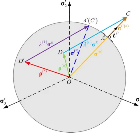
2) We check whether the total stress σ n

 

x,t exceeds the von Mises yield surface at every Gauss point in the body. As illustrated in Fig. 2, the sum of the residual stress vector

OD (ρ x

 

,t ) and the fictitious elastic stress vector DC ( k _{σ x}E

 

,_{t ) is the total stress}

vector OC (σ n

 

x,t ). The part in excess of the von Mises yield surface is the

compensation stress vector AC (σC n

 

x,t ) which is calculated by the following formulae:  

_{ }

 

_{ }

 

_{ }

 

_{ }

 

_{ }

 

_{ }



 

 



 

_{ }





, , , , , , , 0 ,

n n n

C n y n y n n n y

t t t

t t t t t             _      _  ，

σ x x σ x

x x x x x (21)

3) Substituting Eq. (21) into (18), the nodal displacement rate u n

 

t is obtained by solving the equilibrium equations in Eq. (22). The residual stress rate can be calculated by Eq.

(23). Then the residual stress ρ n

 

x,t for the next load vertex can be updated by Eq. (24).  

_{ }

 

_{ }

 

_{ }

, ,

n k T E T C n

V V

t  t dV t dV

 

_

 

_



K u B σ x B σ x (22)

 

_{ }

 

_{ }

 

_{ }

 

_{ }

, , ,

n n k E C n

t    t  t  t

ρ x D B u σ x σ x (23)

 _n

_

_,

_

 _n

_{ }

_, t t  _n

_{ }

_,

t

t  t t 



 t dt

ρ x ρ x ρ x (24)

4) Repeat steps 1-3 for every load vertex.

5) Check the convergence of the value of compensation stress, and repeat the steps 1-4 till

[image:11.595.183.410.75.290.2]

Fig. 2 von Mises yield surface and stress superposition schematic in the deviatoric plane

According to the theorem on existence and uniqueness of a steady stress cycle by

Gokhfeld and Cherniavsky [59], the above procedure will evaluate a steady cyclic stress

state of the structure, and the evolution of compensation stress σ xC

 

,t is also obtained. It should be noted that although the value of σ xC

 

,t may be different from that of

 

,

p

t



D ε x , they are going to vanish at the same time if it happens. Thus, the compensation

stress can be considered as a symbol for estimating whether the structure shakes down, i.e.,

whether the structure responds to the subsequent cyclic loads in a purely elastic manner.

4 Numerical algorithm of the SCM for shakedown analysis

As discussed in Sect. 2, the shakedown behavior of a structure subjected to repeated loads

varying arbitrarily in a load domain can be determined by estimating the behavior of the

structure under a specified loading path which includes all the load vertices, and the existence

of the steady cyclic stress state of a structure with the elastic-perfectly plastic material

obeying the Drucker’s postulate is demonstrated. Instead of using a standard elastic-plastic

finite element analysis, an approximated steady cyclic stress state is assessed by using the

SCM, as elaborated in Sect. 3.

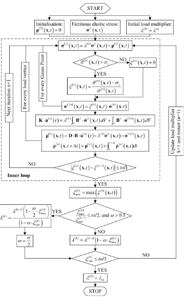
In this section, a numerical procedure well suitable for shakedown analysis is proposed by

process, and the flowchart of the procedure is illustrated in Fig. 3.

[image:12.595.120.479.100.682.2]

4.1 Evaluation of an initial load multiplier

The numerical procedure commences by calculating the fictitious elastic stress field σ xE

 

,t at each extreme point in the specified loading path and by constructing an initial load

multiplier ini. The fictitious elastic stress field can be easily obtained via the elastic finite element analysis. However, the initial load multiplier must be chosen as a value above the

shakedown limit, from which the decreasing load multiplier may be generated after each outer

iteration. According to the description in Ref. [24], the upper bound load multiplier

 

   

1 ini 1 , , m y i V i m E E i i V i dV

t t dV

             _     









x

σ x ε x

(25)

must be an appropriate initial load multiplier. Here, ε xE

 

,t_i is the elastic strain

corresponding to the fictitious elastic stress σ xE

 

,t_i at load vertex t_i, m is the number of

the load vertices, and _i

 

x is the effective strain of E

 

,

i

t

ε x .

4.2 The proposed numerical procedure for shakedown analysis

As illustrated in Fig. 3, the procedure consists of two iteration loops. The inner one controlled

by iteration n is used to obtain the approximately steady cyclic stress, and the outer one

controlled by iteration k is used to calculate the shakedown load multiplier.

For the inner loop, the value of  n

 

x,t (Eq. (21)) is examined:  

_{ }

 1

_{ }

, , 1

n n

t t tol

 _  _

x x (26)

where tol1 is a tolerance parameter which dynamically reduces from 10-3 to 10-4 according to

the value of  n

 

x,t . The maximum value of  n

 

x,t at all the Gauss points for all load vertices is updated at the end of each loading cycle, that is

 



 

_{ }



max max ,

k n

t

   x (27)

Before calculating the load multiplier by the following expression:

   1



 



max 1

k k k

 _  _{ } 

(28)

where  is a convergence parameter with an initial value 0.1~0.5, k1 is the previous

load multiplier and  k is the updated load multiplier, a probable overshooting below shakedown limit will be examined by the following judgment:

 

max1 max

2 and 0.1

k k tol

 _

   ,  (29)

where tol2 usually takes 0.1~0.2; the initial value of _max 0 is 1.0. If Condition (29) is satisfied, the previous load multiplier must be modified by

       





1 max max 1 2 1 k k k k         _{ }      

  (30)

and then the convergence parameter  is halved:

2



 (31)

In final, a desired tolerance tol3 (e.g. 10-4~10-3) is given to estimate whether _max k approaches to zero or not

  max 3

k

tol

  (32)

If Condition (32) is satisfied, it means that the calculated load multiplier becomes the

shakedown limit multiplier _sh, i.e.

  sh

k

  (33)

otherwise, a new outer iteration starts and the inner iteration number resets to 1. In fact, the

criterion shown in Condition (32) is equivalent to the following form:

        1 max 1 k k k k   _{ }     _{ } (34)

where the value of  is not more than 0.5. Thus, the relative error of the calculated

4.3 Convergence and accuracy considerations

An iterative strategy shown in Eq. (28) will allow the proposed procedure to produce a

sequence of decreasing cyclic loading solutions and to end up with the limiting value of

loading parameters at which shakedown takes place. The relevant mathematical proof on the

uniqueness of stress state at the limiting cycle has been presented by Gokhfeld and

Cherniavsky [59]. Thus, if the iterative control technique and some tolerance parameters are

adopted appropriately in the SCM procedure, a series of decreasing load multipliers will

approach smoothly to the shakedown limit multiplier.

The value of tol1 used to control and stop the inner loop is a key factor that influences the

accuracy and efficiency of the algorithm. Considering that the accuracy of the calculated

shakedown limit multiplier is mainly determined by the finally convergent solution and has

little relation to the solution in the intermediate process, a dynamically varying value of tol1 is

used to balance the accuracy and the efficiency. A final value of tol1 10 4 proves enough for a good calculation accuracy of the steady stress cycle.

The iteration strategy shown in Eq. (28) with 0.5 might not strictly prohibit the load multiplier from overshooting below the target solution at shakedown. To deal with this

problem, the numerical scheme shown through Eqs. (29)-(31) is followed, and then even

though the overshooting might still occur, its value must be small enough to be ignored. Once

Condition (29) is satisfied, the calculated load multiplier will increase until above the

shakedown limit multiplier, and then the iterative process continues. The described

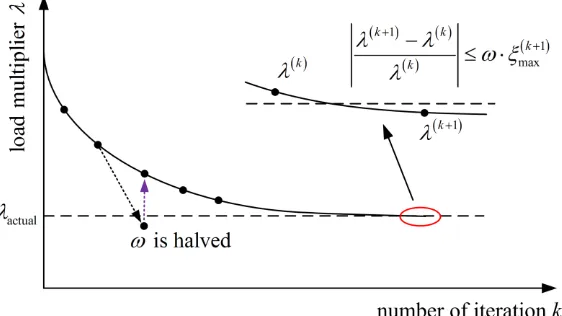
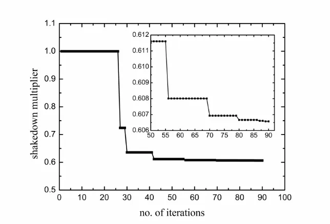
convergence procedure of the SCM for shakedown analysis is vividly depicted in Fig. 4. By

doing so, the method can ensure that the load multiplier approaches to the actual shakedown

limit multiplier _actual from above. Since the adopted shakedown criterion is based on the Melan’s static shakedown theorem and all the conditions of the static theorem are satisfied

when the iterative procedure converges, the calculated shakedown limit multiplier in this

Fig. 4 Convergence procedure of the SCM for shakedown analysis

5 Numerical examples

A significant advantage of the provided method is its ability to be implemented into

commercial finite element software that have the facility to allow the users to establish finite

element models easily and conveniently. The described numerical algorithm in Sect. 4 has

been implemented into ABAQUS [63] via user subroutines UAMT and URDFIL. In order to

illustrate the performance of the present algorithm, three numerical examples of limit and

shakedown analysis are considered. It is mentioned here that limit analysis is considered as a

special case of shakedown analysis when the number of load vertices is reduced to one.

In all examples, the materials are assumed homogeneous, isotropic and elastic-perfectly

plastic with the von Mises yield criterion. All material parameters are constant over time and

independent of temperature. All the calculations are carried out on the personal computer with

16 GB RAM and Intel Core i7 at 3.39 GHz using single processor.

5.1 Square plate with a circular central hole

Fig. 5 shows a square plate with a circular central hole subjected to biaxial loads P1 and P2,

which is a common benchmark example for numerical limit and shakedown analysis

[24,26,28,30,31,38,41,44,55,64-70]. The mechanical material data are given in Table 1. The

ratio between the diameter D of the circular hole and the length L of the plate is 0.2. The ratio

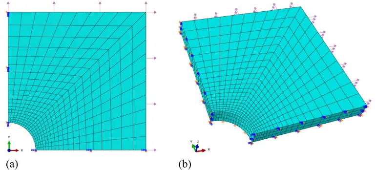
[image:16.595.159.440.78.236.2]

established for the analysis. Since the thickness d of the plate is much smaller than its length L,

both a plane stress problem and a three-dimensional problem are analyzed here. The 2D and

3D finite element models of the plate are shown in Fig. 6. Four hundred 8-node quadratic

plane stress elements (ABAQUS CPS8) with 3×3 Gauss integration points are used for the

plane stress problem in Fig. 6(a), and twelve hundred 20-node quadratic brick elements

(ABAQUS C3D20) with 3×3×3 Gauss integration points are used for the three-dimensional

problem in Fig. 6(b).

Fig. 5 Geometry of the holed plate under biaxial loading

Fig. 6 Finite element models: (a) for the plane stress problem; (b) for the three-dimensional

[image:17.595.196.397.248.471.2] [image:17.595.105.490.523.697.2]

Table 1 Material properties of the plate

Young’s modules E (GPa) Poisson’s ratio v Yield stress _y (MPa)

200 0.3 360

This benchmark problem has been studied by several authors, since it was first

investigated by Belytschko [67]. Some comparative studies have been presented in their

literatures, such as [24,28,30,31,38,44,55,69,70]. As a result, there is no exact solution that is

generally accepted and the shakedown load is relevant to the loading mode. So four different

loading histories are considered, as illustrated in Fig. 7. For loading path a, P1 and P2 vary

independently. For loading path b, P1 and P2 vary proportionally. For loading path c, P1 keeps

constant and P2 varies from nil to a certain value. For loading path d, P1 keeps constant and P2

varies from minus to plus.

Fig. 7 Four loading histories for shakedown analysis: (a) loading path a; (b) loading path b;

(c) loading path c; (d) loading path d

5.1.1 P1 and P2 vary independently

The plate is subjected to biaxial uniform loads P1 and P2 that vary independently in the

following ranges:

1 1 0 0 P P

[image:18.595.136.459.341.576.2]

The shakedown limits calculated by the SCM are compared to the mentioned results

[24,26,28,30,31,38,41,44,64-70] for the three special loading cases ₂0, ₂0.5₁ and 2 1

  in Table 2. The values of shakedown limits in Table 2 are normalized with the ratio

0 y

P  . As explained in Ref. [30], the partly-analytical solution by Zhang [68] can be

[image:19.595.87.512.211.717.2]

considered as the reference solution.

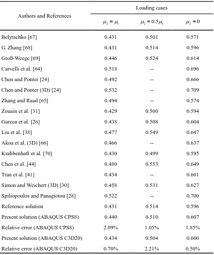
Table 2 Comparison of different numerical results for shakedown analysis

Authors and References

Loading cases

2 1

  ₂0.5₁ ₂0

Belytschko [67] 0.431 0.501 0.571

G. Zhang [68] 0.431 0.514 0.596

Groß-Weege [69] 0.446 0.524 0.614

Carvelli et al. [64] 0.518 -- 0.696

Chen and Ponter [24] 0.492 -- 0.666

Chen and Ponter (3D) [24] 0.532 -- 0.709

Zhang and Raad [65] 0.494 -- 0.574

Zouain et al. [31] 0.429 0.500 0.594

Garcea et al. [26] 0.438 0.508 0.604

Liu et al. [38] 0.477 0.549 0.647

Akoa et al. (3D) [66] 0.466 -- 0.637

Krabbenhøft et al. [70] 0.430 0.499 0.595

Chen et al. [44] 0.480 0.553 0.649

Tran et al. [41] 0.434 -- 0.601

Simon and Weichert (3D) [30] 0.458 0.531 0.627

Spiliopoulos and Panagiotou [28] 0.522 -- 0.700

Reference solution 0.431 0.514 0.596

Present solution (ABAQUS CPS8) 0.440 0.510 0.607

Relative error (ABAQUS CPS8) 2.09% 1.05% 1.85%

Present solution (ABAQUS C3D20) 0.434 0.504 0.600

Relative error (ABAQUS C3D20) 0.70% 2.21% 0.50%

(3D) denotes that the results are obtained from three-dimensional model, and the other results are

As we can see, the different numerical results in Table 2 show that our solution is in great

agreement with the values from the reference solution where the maximum relative error is

only 2.09% for plane stress problem and 2.21% for three-dimensional problem. It should be

noted that there is a relatively large range among those numerical results. The discrepancy is

attributed not only to the different methods but also to the different types of finite elements

and sizes of the element meshes used for the initial elastic solution. A simple way to illustrate

the influence of finite elements is the existing difference of the maximum elastic stress

between in this paper and in Ref. [24] under same single loading P1. The maximum elastic

stress is 3.297P1 when the finite element meshes in this paper are used but is 2.891P1 when

the element meshes in Ref. [24] are used. What’s more, the maximum relative error is only

0.49% between the present solution for plane stress problem and the solution by Garcea [26],

whose finite element model has the most approximate mesh size with the finite element model

in Fig. 6(a).

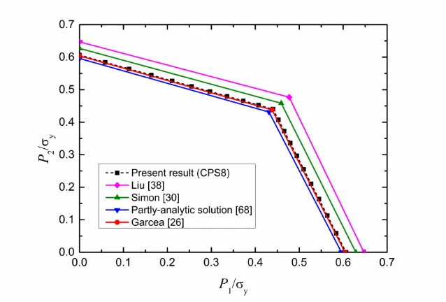
After calculating the shakedown limits for various ratios of  _{1 2} by using the SCM, the shakedown domain was obtained. As illustrated in Fig. 8, these points of shakedown limits

align in two straight-line segments and the results coincide well with the reference solution.

Furthermore, the shakedown boundary in Fig. 8 is dominated by alternating plasticity.

[image:20.595.137.456.492.708.2]

under loading case ₂0. The horizontal line segment in the Fig. 9 indicates that the procedure is being carried out for the steady cyclic state, and the decreasing values indicate

the procedure is being carried out for the iterative process of the load multipliers. Although,

with the increase of iteration number, the calculated load multipliers do not strictly decrease

monotonically, the solutions converge to the stable one which is the actual solution with a

specified tolerance (10-4) by using the reasonable iterative control technique.

The crucial idea of the Melan’s theorem for shakedown analysis is to find an optimal

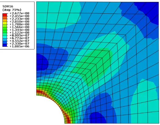
time-independent self-equilibrated residual stress field. As a result, a final residual stress field

of the holed plate is shown in Fig. 10. It should be noted that, the calculated residual stress

field by the SCM is non-unique and related to the initial load multiplier, but the calculated

shakedown limit multipliers are the same for different initial load multipliers, which verifies

the discussions in Sect. 2.3.

In order to illustrate the efficiency of the proposed procedure for shakedown analysis, the

computing time for some cases with different number of finite elements is compared in Table

3. For the finite element model with 4008-node quadratic plane stress elements in Fig. 6(a),

the amount of CPU time ranges from 6 s for the case of ₂0 to 11 s for ₂ ₁. Specially, for a large-scale three-dimensional finite element problem with 20000 20-node

quadratic brick elements (ABAQUS C3D20), the computing time is only 2558 s.

[image:21.595.136.458.507.726.2]

[image:22.595.167.429.78.284.2]

Fig. 10 Equivalent residual stress field of the holed plate for loading case a (₂ 0)

Table 3 Computing time for shakedown analysis of the holed plate

Finite Elements Loading cases 1 2 CPU time (s)

400 CPS8 20 0.607 0 6

400 CPS8 12 0.440 0.440 11

400 CPS8 11.252 0.466 0.373 10

1200 C3D20 12 0.434 0.434 131

20000 C3D20 12 0.429 0.429 2558

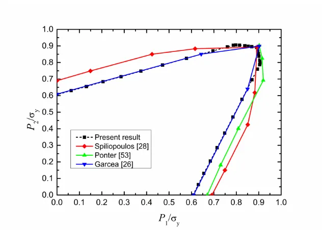
5.1.2 P1 and P2 vary proportionally

The shakedown analysis of the holed plate with P1 and P2 varying proportionally is also

considered by using the SCM. The same case has already been analyzed by some authors

[26,28,53] and the present results are compared in Fig. 11. It is worth noting that, for the

present results in Fig. 11, the straight-line portion of the shakedown boundary curve is

[image:23.595.138.454.73.299.2]

Fig. 11 Shakedown domain of the square plate for loading path b

5.1.3 P1 is constant and P2 is cyclic

The SCM is used to calculate the shakedown limits of the plate under loading path c and

loading path d (Fig. 7). These two shakedown problems have been considered by Chen and

Ponter [55]. In order to exclude the discrepancy of the mesh discretization, the comparison of

the calculated results by the SCM and those by the LMM is based on the same finite element

model. Fig. 12 and Fig. 13 give the shakedown domains of the square plate under loading

path c and loading path d, respectively. Each figure of them includes the shakedown domains

by the SCM with two different kinds of mesh discretization, the shakedown domain by the

LMM, and the results from Ref. [55]. The mark “mesh 1” in the legend denotes that the mesh

displayed in Fig. 6(a) is used, and the mark “mesh 2” denotes that the mesh from Ref. [55] is

used.

We can observe from Fig. 12 and Fig. 13 that the results obtained by the SCM and the

LMM agree very well with each other for the same mesh model, which verifies the validity of

the two methods. Nevertheless, for the different mesh models, there are obvious differences in

the plateaus of shakedown boundary curves, while the rest of the curves are very agreeable.

The differences are in fact due to the different failure modes of the structure. In both Fig. 12

alternating plasticity, for which the shakedown limit is relevant to the local maximum stress.

Thus, the difference in the local maximum stress due to the inconsistent mesh leads to the

different shakedown limits. However, if the structure fails due to incremental plasticity, as is

the rest portion of these shakedown boundary curves in Fig. 12 and Fig. 13, the shakedown

[image:24.595.139.456.201.415.2]

limit is insensitive to the mesh.

[image:24.595.139.455.448.670.2]

Fig. 12 Shakedown domains of the square plate for loading path c

Fig. 13 Shakedown domains of the square plate for loading path d

In the above examples, the shakedown domains are all obtained by the SCM under

those by other methods.

5.2 Defective pipeline

Pipelines, which are generally made up of ductile steel, are widely used in various fields, such

as petrochemical industry, energy, nuclear industry, and electric power engineering, etc.

During their operation, many defects such as part-through slots can be produced by

mechanical damage, corrosion or abrading surface cracks. These defects may jeopardize the

integrity (i.e. reduce the load-carrying capacity) of pipelines and sometimes even lead to

severe industrial accidents. The integrity assessment of pipelines with part-through slots is a

very important research subject with significant and extensive application background in the

industry. Plastic limit and shakedown analysis plays a significant role in the integrity

assessment of defective pipelines. In this paper, through some computational examples and

analyses, the effects of small and large area slots on the load-carrying capacity of pipelines are

investigated and evaluated.

These examples adopted here are three-dimensional defective pipelines under internal

pressure and axial tension [24]. The geometry of the structure is shown in Fig. 14. The

mechanical material data are given in Table 4. It should be noted that the applied total axial

loads consist of the independent axial tension N and the additional axial tension N1 induced by

independent internal pressure P. The additional axial tension N1 is equal to P R _i2, where Ri

is the inner radius of pipeline. Here a small spherical slot and a large area slot are considered

for limit and shakedown analyses. The geometric parameters of the slotted pipelines are

presented in Table 5.

Fig. 14 Geometry of pipeline with part-through slot subjected to internal pressure and axial

Table 4 Material properties of pipelines

Young’s modules E (GPa) Poisson’s ratio v Yield stress y (MPa)

200 0.3 245

Table 5 Geometric parameters of pipelines with different defect types (mm)

Defect type Ri Ro L α A1 A B C

Small slot 17 21 250 0 2 2 2 2

Large area slot 17 21 250 45° 2 10 2 2

Due to the symmetry of the structure and the loading, only a quarter of the defective

pipeline is considered. The corresponding displacement constraints are imposed on the

symmetric boundaries. The 3D finite element mesh discretization of the pipeline is shown in

Fig. 15, where the 20-node quadratic brick elements (ABAQUS C3D20) with 3×3×3 Gauss

integration points are used. In order to optimize the efficiency and accuracy of the calculation,

the finite elements around the slots should be distributed appropriately to make them as much

neat and fine as possible. The numbers of finite elements used to discretize the pipelines with

a small slot and with a large area slot are 1905 and 1658, respectively.

The SCM is used to calculate the shakedown limits of the defective pipeline under axial

tension and internal pressure with five different loading paths, as shown in Fig. 16. For

loading path a, the single load N varies from nil to a certain value. For loading path b, the

single load P varies from nil to a certain value. For loading path c, three vertices of the

loading path are included, in which the maximum independent axial tension N (replaced by

the equivalent uniform tension) is four times of the maximum internal pressure P. For loading

paths d and e, the single load N and P keep certain value, respectively. The loading paths d

and e are used to calculate the limit loads of the defective pipeline subjected to independent

[image:27.595.152.447.80.364.2]

Fig. 15 3D finite element meshes for slotted pipeline: (a) with a small slot; (b) with a large

area slot

Fig. 16 Five different loading paths for shakedown analyses

As we all know, the shakedown limit of elastoplastic structure under proportional load is

the minimum one of its plastic limit load and its double elastic limit load. Thereby, the

shakedown limit of the defective pipeline can be determined via an elastic-plastic incremental

analysis and a linear elastic analysis using the finite element software ABAQUS.

[image:27.595.142.456.416.623.2]

Ponter [24], and was used for the shakedown and limit analyses of three-dimensional

structures. In this paper, the shakedown and limit loads of the defective pipelines under axial

tension and internal pressure with the five loading paths shown in Fig. 16 are calculated by

the above three different methods, i.e., the SCM, the method of ABAQUS and the LMM.

It should be explained that the defective pipelines considered here have the same

geometry, mechanical material data and load conditions as those in Ref. [24], but are different

in mesh discretization with the reference. In order to compare the performance of the SCM

and the LMM reasonably, the same finite element model must be considered. The present

numerical results by the LMM for defective pipelines are based on the finite element models

in Fig. 15, which has a slight difference with the results in Ref. [24].

Table 6 and Table 7 show the numerical results of shakedown analysis for the pipelines

with a small slot and with a large area slot, respectively. It can be seen that the shakedown

limits obtained by the SCM are in excellent agreement with the solutions by the method of

ABAQUS and the LMM. As a general result, the linear matching method is an upper bound

method, by which the calculated shakedown loads are bigger than that by the other two

methods. For the pipeline with a large area slot under the five different loading histories, the

maximum deviation of the shakedown loads between the results calculated by the SCM and

that by the method of ABAQUS is 2.9%.

Table 6 Shakedown limit for the pipeline with a small slot under five different loading paths using three different methods

Loading

paths

Shakedown limit (MPa) for the load domain

SCM ABAQUS LMM

Case a (0,0), (229.6,0) (0,0), (229.8,0) 1 (0,0), (229.7,0)

Case b (0,0), (0,56.8) (0,0), (0,57.0) 1 (0,0), (0,57.1)

Case c (0,0), (172.0,0), (0,43.0) --- (0,0), (173.3,0), (0,43.32)

Case d (0,0), (242.1,0) (0,0), (244.5,0) (0,0), (244.8,0)

Case e (0,0), (0,57.4) (0,0), (59.1,0) (0,0), (0,59.7)

[image:29.595.137.455.346.568.2]

Table 7 Shakedown limit for the pipeline with a large area slot under five different loading

paths using three different methods

Loading

paths

Shakedown limit (MPa) for the load domain

SCM ABAQUS LMM

Case a (0,0), (168.7,0) (0,0), (168.7,0) 1 (0,0), (169.9,0)

Case b (0,0), (0,38.4) (0,0), (0,39.3) 2 (0,0), (0,39.5)

Case c (0,0), (142.8,0), (0,35.7) --- (0,0), (143.8,0), (0,35.9)

Case d (0,0), (208.2,0) (0,0), (212.6,0) (0,0), (215.3,0)

Case e (0,0), (0,38.7) (0,0), (0,39.3) (0,0), (0,39.5)

( ) 1, the superscript indicates the shakedown load is determined by the double elastic limit load. ( ) 2, the superscript indicates the shakedown load is determined by the plastic limit load.

Fig. 17 Convergence procedure of the SCM towards the shakedown load for the defective

[image:30.595.161.435.71.268.2]

Fig. 18 Equivalent residual stress field of the defective pipeline with a large area slot under

loading case b

Under the proposed five loading paths, all the calculations for shakedown analysis of

these defective pipelines have good convergence condition. As an example, the convergence

procedure of the SCM towards the shakedown load for the defective pipeline with a large area

slot under loading path b is shown in Fig. 17. Moreover, this case generates the maximum

number of iteration for the five cases considered here. It should be noted that the increase of

the shakedown multiplier during the process of the iteration indicates that an overshooting of

the shakedown limit has occurred in the previous iteration. However, the shakedown

multiplier still converges to the final result by halving the convergence parameter . The

final equivalent residual stress field is shown in Fig. 18.

Assuming the axial tension and internal pressure vary independently, the SCM is used to

calculate the shakedown limits of the pipeline for various ratios of the applied axial tension

and internal pressure. Then shakedown domains of the defect-free pipeline as well as the

defective pipelines with a small slot and with a large area slot are presented in Fig. 19.

In order to demonstrate the computational efficiency of the SCM for complex

three-dimensional problem, the LMM and the step-by-step procedure are also used to

calculate the shakedown load of the pipeline for same ratios of the applied axial tension and

shakedown analysis of the defective pipelines under three load domains by the SCM, the

LMM and the step-by-step procedure are compared in Table 8. It can be seen from Table 8

that, with necessary accuracy of calculations (see Fig. 19), the CPU time by the step-by-step

procedure is 20 times more than that by the SCM while the computational efficiency of the

SCM is higher than that of the LMM.

As a by-product, the strain history of the pipeline under cyclic loading is also obtained

from the incremental elastic-plastic calculation. In Fig. 19, the load conditions marked with

capital letters “A” and “B” are acted on the defective pipelines with a small slot while the

load conditions marked with capital letters “C” and “D” are acted on the defective pipelines

with a large area slot. Fig. 20 shows the effective plastic strains of the pipeline with a small

slot over the first 10 load cycles for point “A” and point “B”. It can be seen that the pipeline

with a small slot exhibits alternating plasticity behavior for point “A” and shakedown

behavior for point “B”. Fig. 21 shows the effective plastic strains of the pipeline with a large

area slot over the first 15 load cycles for point “C” and point “D”. The pipeline with a large

area slot shakes down after 11 load cycles for point “D”, but failures due to the incremental

plasticity mechanism for point “C”.

Fig. 19 Shakedown domains of the defect-free pipeline and the defective pipelines with a

[image:31.595.138.453.474.697.2]

[image:32.595.83.510.120.249.2]

Table 8CPU time (s) for shakedown analysis of the defective pipeline under different load

domains by the SCM, the LMM and the step-by-step procedure

Load domains (MPa) 0 300sin 0 100cos

N P

 

 

 

With a small slot With a large area slot

SCM LMM Step-by-step SCM LMM Step-by-step

θ = 30°

324 660 6211 319 480 6735

θ = 45°

291 635 5984 303 493 6612

θ = 60°

325 611 6121 311 562 6786

Fig. 20 Effective plastic strains of the pipeline with a small slot over the first 10 load cycles

for point “A” and point “B”

[image:32.595.143.454.161.470.2] [image:32.595.159.437.526.719.2]

5.3 Header component

The third numerical example is a header component, which is typically used in an advanced

gas-cooled reactor (AGR) power plant. In the cooling and reheating process of the AGR, the

header often experiences complex load conditions due to its interaction with the rest of the

piping system. Here, a schematic of the header component is shown in Fig. 22, where the

main pipe has two vertical branch pipes with the same geometric dimension. In the present

paper, some typical loading cases are considered and the shakedown boundaries of the header

component under different load domains are calculated by the SCM.

The header component is depicted by some characteristic dimensions in Fig. 22, and the

values of these dimensions are listed in Table 9. For the convenience of calculation, the

material properties are assumed constant over time and independent of temperature. The

detailed mechanical material data of the header component are given in Table 10.

[image:33.595.121.475.394.596.2]

Fig. 22 Geometry of the header component

Table 9Geometric parameters of the header component (mm)

Dimension A B C D E F G

[image:33.595.88.508.666.716.2]

Table 10 Material properties of the header component

Young’s modules E (GPa) Poisson’s ratio v Yield stress y (MPa)

200 0.3 165

Three groups of different loads are applied to the header component, whose fundamental

loads are listed in Table 11. For the first group, the internal pressure P_i3.64 MPa is applied to all internal surfaces of the structure, and the internal pressure leads to additional

tensions at ends of the main and branch pipes. For the second group, the axil force F, which

has been replaced by the equivalent uniform pressure P_F 40 MPa, is applied to the outboard main pipe end. For the third group, the bending moment M_mx 240 kN m and

160 kN m

my

M    are applied to the outboard main pipe end, and the bending moment 9.6 kN m

bz

M    is applied to the inboard branch pipe end. It should be noted that these three bending moments are assumed to vary synchronously. Hence, the amplitudes of the

three group loads can be determined by three dimensionless load factors, i.e. P0, F0 and M0.

In order to balance the efficiency and accuracy of the calculation, the 20-node quadratic

brick elements with reduced integration (ABAQUS C3D20R) are used to discretize the

structure, and the meshes around the area of stress concentration are refined properly. As

shown in Fig. 23, the mesh discretization consists of 27540 elements and 139251 nodes. The

reference points and kinematic coupling constraints are used to apply the bending moments

[image:34.595.87.512.604.705.2]

and boundary conditions to the model.

Table 11 Fundamental loads applied to the header component

Load

P0 F0 M0

Internal pressure Pi (MPa)

Main tension Pma

(MPa)

Branch tension Pbr

(MPa) F P (MPa) mx M

( kN m )

my

M

( kN m )

bz

M

[image:35.595.154.444.74.274.2]

Fig. 23 Finite element model of the header component

Here, two types of combinations of two loadings are considered.

(1) Combination I

We consider the load factor F0 equals to zero, and then the load domains of interest are

dominated by the load factor P0 and M0, as displayed in Fig. 24.

Fig. 24 Four different load domains for combination I: (a) domain a; (b) domain b; (c)

domain c; (d) domain d

The SCM is used to calculate the shakedown limits of the header component for various

loading cases. As results, four shakedown boundaries corresponding to the four load domains

are presented in Fig. 25. For the load domains a and b, alternating plasticity is the critical

[image:35.595.168.428.415.619.2]

alternating plasticity (curve 1 and curve 4 in Fig. 25) and incremental plasticity (curve 2 and

curve 3 in Fig. 25). It should be noted that the load history is dominated by one parameter in

the load domain b, thus, the shakedown load is the double elastic limit load. For comparison,

the elastic boundary is also presented in Fig. 25. The shakedown boundary curve for the load

domain b has the same shape and twice values in amplitude as the elastic boundary curve.

Fig. 25 Shakedown domains of the header component for combination I: P0 versus M0

[image:36.595.157.435.204.453.2]

(2) Combination II

[image:36.595.171.424.525.724.2]

Here, we consider that the load factor M0 equals to zero. The load domains of interest are

dominated by the load factor P0 and F0, as displayed in Fig. 26.

The SCM is used to calculate the shakedown limits of the header component. Four

shakedown boundaries corresponding to the four load domains and the elastic boundary are

all presented in Fig. 27. It is obvious that the shapes of the four calculated shakedown

boundaries for the combination II are very similar to these for the combination I. Furthermore,

the same critical failure modes dominating the shakedown boundaries are observed for the

[image:37.595.157.435.274.523.2]

two types of load combinations.

Fig. 27 Shakedown domains of the header component for combination II: P0 versus F0

To the authors’ best knowledge from literatures, until now, the shakedown problem of this

comparable scale has never been solved before. In this paper, about one hundred calculations

have been completed to demonstrate the performance of the SCM for shakedown analysis of

the large-scale header component under various load conditions. All iterative procedures of

the SCM for shakedown analysis present good convergence. The convergence tolerances are

all met within 270 increments, and the CPU time is not more than 40 minutes. The equivalent

residual stress field of the header component is also obtained conveniently, as shown in Fig.

Fig. 28 Equivalent residual stress field of the header component

6 Discussion and conclusions

A novel direct method so-called the stress compensation method (SCM) for the application of

limit and shakedown analysis to large-scale elastoplastic structures has been proposed, where

a two-level iterative procedure is performed by a series of linear elastic finite element

analyses and the conventional mathematical programming problem does not need to be solved.

The global stiffness matrix is decomposed only once during the whole procedure, which

contributes to the high efficiency of the SCM, especially for large-scale problems. By

adopting an efficient and robust iteration control technique, the convergence and the accuracy

of the SCM are ensured. Since all the conditions of the static shakedown theorem can be

satisfied when the iterative process converges, the shakedown limit calculated by the SCM is

a lower bound approximate to the actual solution with predefined tolerance.

Comparing the SCM with the residual stress decomposition method for shakedown

(RSDM-S) [28], one may note that the RSDM-S decomposes the residual stresses into Fourier

series with respect to time and thus requires many time points inside the cycle to represent the

applied loading. After each iteration of the numerical procedure, these Fourier coefficients

need to be calculated at all Gauss points by performing the numerical integration of residual

[image:38.595.135.456.73.300.2]