A Double-Error Correction Computational Model of Learning

(1)

City, University of London Institutional Repository

Citation:

Kokkola, N. (2017). A Double-Error Correction Computational Model of Learning. (Unpublished Doctoral thesis, City, University of London)

This is the accepted version of the paper.

This version of the publication may differ from the final published

version.

Permanent repository link:

http://openaccess.city.ac.uk/18838/

Link to published version:

Copyright and reuse: City Research Online aims to make research

outputs of City, University of London available to a wider audience.

Copyright and Moral Rights remain with the author(s) and/or copyright

holders. URLs from City Research Online may be freely distributed and

linked to.

City Research Online: http://openaccess.city.ac.uk/ [email protected]

(2)

A Double-Error Correction

Computational Model of Learning

Niklas H. B. Kokkola

Supervisor: Dr. Eduardo Alonso

First Supervisor

Dr. Chris Child

Second Supervisor

Dr. Esther Mondragón

External Supervisor

This dissertation is submitted for the degree of

Doctor of Philosophy

City, University of London

Department of Computer Science

(3)

(4)

List of figures

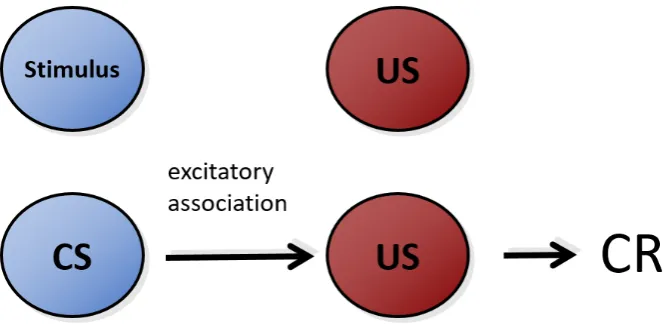
1.1 Conditioning. The pairing of a stimulus with a US engenders the formation of an excitatory association from the (now) conditioned stimulus to the US. This association invokes the production of a conditioned response (CR). . . 36 1.2 The comparator hypothesis of Miller & Matzel (1988) postulates that the

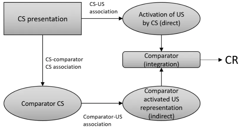
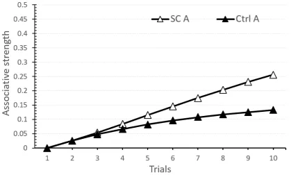
presentation of a CS invokes both a direct US representation, and an indirect activation of the US representation through comparators. These two pathways compete with one another to determine the net CR produced by the CS. . . 45 1.3 Simulation of the TD model using the TD simulator (Gray, J., Alonso, E.,

Mondragón, E., and Fernández, 2012). Displayed is the result of simulating acquisition for a reinforced serial compoundA→B→+(Group SC) com-pared toA→+(Group Ctrl). Group SC displays higher-order conditioning. 49 1.4 Simulation of the REM model using the REM simulator (Ghorashi, A.,

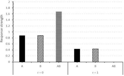
Mon-dragón, E. and Alonso, 2017). Results of the conceptual design 20A+/20B+ (random) followed by test trials for compound AB, withr=0 andr=1. . 54 1.5 1) An elemental connectionist structure. CSs are directly associated with the

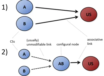
occurrence of the US. 2) A configural connectionist structure. CSs activate a configural representation, which in return enters into association with the US. 56 1.6 Simulation of the Pearce model using the Pearce Model Simulator

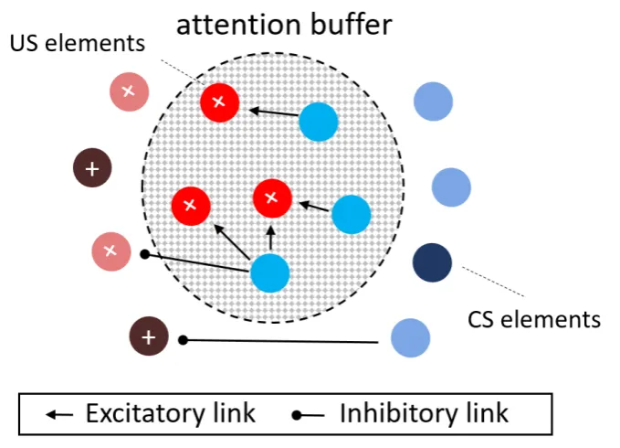
(Gho-rashi, A., Mondragón, E. and Alonso, 2017). Results of a biconditional discrimination are displayed. . . 58 1.7 The fixed-capacity attentional buffer of the Harris (2006) model. Elements

(9)

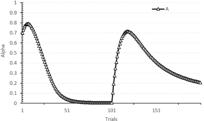
1.8 Simulation of the Pearce-Hall model using the Pearce-Hall Model Simulator (Grikietis, R., Mondragón, E., and Alonso, 2016). Alpha value of cue A in a simulation of 100A+/100A- is displayed. . . 67 1.9 (Hall and Rodriguez, 2010) postulates that pre-exposure induces the

forma-tion of aCS− ¬U Slink, that subsequently interferes with the CS-US link formed during acquisition. . . 69 1.10 Top left: SOP activation states: I, A1, and A2 are respectively inactive, active,

and associatively activated or decayed activation states, and p1 and p2 are respectively rates by which inactive elements can be activated into A1 or A2 states. pd1 and pd2 are respectively rates at which A1 elements decay into the A2 states, and A2 elements decay into the inactive state. Top right: SOP learning rules. Bottom Right: Dickinson & Burke SOP learning rules. Bottom Left: Holland SOP learning rules. . . 77 1.11 Replay model of (Ludvig et al., 2017). Previously experienced stimulus

con-tingencies are replayed by the animal during periods of reduced stimulation, such as during an ITI. . . 83 1.12 The Double Error Model simulator GUI. . . 86 2.1 A stimulus is constituted by elements unique to it, common elements shared

with other stimuli, and the elements respective activation state. . . 92 2.2 Conceptual representation of the elemental network structure of the DE

model. . . 93 2.3 Time-waves are skewed to the right, have a specified peak t and denote the

probability that a given element belonging to this temporal cluster is active at a given time-point. . . 95 2.4 The presence of a stimulus produces a cascade of time-waves in proportion to

its length. Each time-wave peaks at a subsequent time-point and its standard deviation is proportional to its mean. A given time-wave gives the activation probability of elements ’belonging’ to the wave. . . 95 2.5 Associative links between stimuli allow stimuli to retrieve the representations

of absent stimuli. This can produce chains of associative retrieval, e.g.

A→B→C, as displayed. . . 97 2.6 Associative activation of one (absent) CS by another (present) CS, after both

(10)

2.7 Total activation of a 10 time-unit CS, with persistent memory trace visible. The probabilistically sampled elements of a stimulus aggregate to constitute the overall activation of a stimulus. . . 100 2.8 The direction of learning between a predictor and outcome in the DE model

is determined by the outcome’s error-term, which is influenced both by the similarity in activation of the predictor and outcome, as well as the total prediction for the outcome by all elements. . . 101 2.9 Asymptote of learning as a distance measure of the activities of the predictor

and outcome. . . 103 2.10 αrvalue of cue A in a simulation of partial reinforcement. Once the moving

average ofα passes a threshold, sufficient evidence has accumulated that the

contingency is inherently random, and thus attention decays. . . 108 2.11 αr value of cue A in a simulation of 50A+/50A-. Theαr value rises at the

beginning of both acquisition and extinction due to the change in contingency producing prediction errors for the outcome. . . 109 2.12 αr values of 10 time-unit CSs with imperfect (10 intermixed A+ and

A-trials) and perfect (10A+ A-trials) predictors of an outcome. The revaluation alpha rises to a higher level for the perfect predictor due to it producing a larger outcome error before the outcome onset. . . 109 3.1 Simulated weights of the CS in the acquisition and extinction procedure with

5, 10, and 20 time-unit CSs. . . 118 3.2 Simulated weights of the CS in the acquisition procedure with forward,

backward, and simultaneous conditions. . . 119 3.3 Simulated weights in the acquisition procedure with forward, backward, and

simultaneous conditions withb=0.0. . . 120 3.4 Simulated CS weights of the CS in the acquisition procedure 10,30,60,120,240

time-unit ITIs and 5 time-unit CS. . . 121 3.5 Simulated context weights in the acquisition procedure with 10, 30, 60, 120,

240 time-unit ITIs and 5 time-unit CS. Longer ITIs lead to context extinction. 122 3.6 1) waves of a 10 time-unit CS with a wave-constant of 1.50. 2)

Time-waves of a 10 time-unit CS with a wave-constant of 15.00. . . 123 3.7 Anticipatory CR after 10 trials of acquisition of a 10 time-unit CS with a

(11)

3.8 Simulation of partial reinforcement with the PH model using the Pearce-Hall Simultator (Grikietis, R., Mondragón, E., and Alonso, 2016), with reinforce-ment ratios of 0.25, 0.5, 0.75, and 1.0. The model is unable to reproduce the effect whereby the asymptote of partial reinforcement is proportional to the ratio of reinforced to non-reinforced trials. . . 125 3.9 Simulated weights of stimulus A in the partial reinforcement design. . . 126 3.10 Simulated weights of stimulus B in the CI procedure for block and intermixed

presentations. . . 129 3.11 Simulated prediction errors of the US in the CI procedure for block and

intermixed presentations. . . 129 3.12 Simulated weights in the second phase of the blocking procedure. . . 131 3.13 Trial-by-trial prediction error for the US in the blocking simulation. . . 132 3.14 Left: Mean percent freezing in the test phase of experiment 1 of Bradfield

& McNally (empirical units adapted from paper), Right: corresponding response strength in the test phase in simulation of Experiment 1. . . 133 3.15 Experiment 1 design of learned irrelevance in Baker et. al. . . 137 3.16 Left: Suppression ratios in experiment 1A of Baker et al. 2003 (empirical

units adapted from the paper) for the acquisition test trials in the third phase, Right: corresponding simulated suppression ratios for the same trials. Average correlationR=0.92. . . 137 3.17 Top: Suppression ratios in experiment 1B of Baker et al. 2003 (empirical

units adapted from the paper) for the retardation test trials in the third phase, Bottom: corresponding simulated suppression ratios for the same trials. Average correlationR=0.54. . . 140 3.18 Simulation weights of CS N to the US in the beginning of the third phase of

the Baker et. al. 2003 learned irrelevance experiment 1A. . . 141 3.19 Empirical (original measurement units) and simulated results during the

conditioning phase of Experiment 3, Channell & Hall, (1983). The left panel is an adaptation of the paper data showing acquisition of a CR in groups Exposed Same, Exposed different, Control Same and Control different. The right panel displays the corresponding simulated results. Average correlation

R=0.97. . . 144 3.20 Acquisition in the context specificity of latent inhibition simulation with the

αr associability disabled. . . 146

(12)

3.22 Acquisition in the context specificity of latent inhibition simulation with 100 trials of context pre-exposure after the CS pre-exposure. The result is a decrease in the latent inhibition of stimulus A. . . 148 3.23 Acquisition in the context specificity of latent inhibition simulation with

pre-exposure in two different contexts. . . 149 3.24 Acquisition in the context specificity of latent inhibition simulation with the

PH model simulator (Grikietis, R., Mondragón, E., and Alonso, 2016). . . 149 3.25 Hall-Pearce effect design, Hall & Pearce 1979. . . 151 3.26 Left: Empirical suppression ratios from phase 2 of Experiment 1, Hall &

Pearce 1979 (original measurement units adapted from the paper) showing the acquisition of a CR in groups Tone-shock, Light-shock, Tone-alone, Right: corresponding simulated suppression ratios for phase 2, average correlationR=0.97. . . 151 3.27 Trial prediction-error for the Tone CS in phase 2 of Hall-Pearce negative

transfer. . . 152 3.28 αrdifferences for the Tone CS in phase 2 of Hall-Pearce negative transfer. 153

3.29 Simulation weights of cue T in the second phase of Hall-Pearce negative transfer, displaying sigmoidal acquisition in the Tone-alone group. . . 153 3.30 Simulation responding in the second phase of the Hall-Pearce design with

either the same context (S) or different context (D). . . 154 3.31 Perceptual Learning design of Blair & Hall, 2003. . . 155 3.32 Left: Combined mean consumption (ml) for BX and CX test trials in

experi-ment 1a of Blair and Hall, 2003 (empirical units adapted from paper). Right: Corresponding simulated mean consumption for BX and CX test trials. . . 156 3.33 Second perceptual learning experiment design. . . 157 3.34 Response strength during Phase 2 of the second PL experiment simulation. 158 3.35 Response strength during Phase 3 of the second PL experiment simulation. 158 3.36 Leung et. al. experiment 3 compound latent inhibition design. . . 160 3.37 Left: Mean percent freezing in the test phase of experiment 3 Leung et.

al. (empirical units adapted from paper). Right: corresponding response strength per trial in the test phase in simulation of experiment 3 of Leung et. al. Average correlationR=0.75. . . 160 3.38 The non-reinforced revaluation alpha,αn, in the simulated third phase

(13)

3.39 Simulation of compound LI with PH model simulator (Grikietis, R., Mon-dragón, E., and Alonso, 2016). . . 163 3.40 Response strength in the test phase of the simulation of SPC. . . 166 3.41 The temporal overlap in activity between cues A and B in phase 1 of the

simulation of SPC. . . 167 3.42 The serial compound presentation of A and B leads to the formation of an

excitatoryB→Alink in phase 1 of the SPC simulation. . . 167 3.43 The retrieval of A by B in the second phase of the SPC simulation invokes

the formation of anA→+link through mediated conditioning. . . 168 3.44 Weights of cue A to the US in the second phase of the simulation of backward

blocking with 5 and 100 trials of AB+ training, 20 acquisition trials, 5 time-unit CS, and 1 time-time-unit US. . . 170 3.45 Weights of cue B to the US in the second phase of the simulation of backward

blocking with 5 and 100 trials of AB+ training, 20 acquisition trials, 5 time-unit CS, and 1 time-time-unit US. . . 170 3.46 Weights of cue A to the US in the second phase of the simulation of backward

blocking with 5 and 100 trials of AB+ training, 20 acquisition trials, 1 time-unit CS, and 1 time-time-unit US. . . 171 3.47 Weights of cue B to the US in the second phase of the simulation of backward

blocking with 5 and 100 trials of AB+ training, 20 acquisition trials, 1 time-unit CS, and 1 time-time-unit US. . . 171 3.48 Weights of cue B to the US in the second phase of the simulation of

unover-shadowing with 20 and 100 trials of AB+ training, 20 acquisition trials, 5 time-unit CS, and 1 time-unit US. . . 173 3.49 Weights of cue A to the US in the second phase of the simulation of mediated

conditioning with 20 and 100 trials of AB training, 20 acquisition trials, 1 time-unit CS, and 1 time-unit US. . . 175 3.50 Weights of retrieved cue B to the US in the second phase of the simulation of

mediated conditioning with 20 and 100 trials of AB training, 20 acquisition trials, 1 time-unit CS, and 1 time-unit US. . . 175 3.51 Design of experiment 4 of Le Pelley & McLaren, 2001. . . 177 3.52 Top: Ratings of target cues after Stage 2 of experiment 4 of Le Pelley

(14)

3.54 Left: suppression ratios in test phase of experiment 2 of Ward-Robinson & Hall for Group VI and Group Ext (empirical units adapted from paper), Right: corresponding simulated suppression ratio. Average correlationR=0.87. . 182 3.55 Negative patterning experimental design of (Whitlow & Wagner, 1972). . . 185 3.56 Left: Responses in the discrimination phase of the negative patterning

ex-periment of Whitlow & Wagner, 1972 (empirical units adapted from paper). Right: Equivalent simulated responses. . . 185 3.57 Left: Mean percentage conditioned responses per compound in the test phase

of the negative patterning experiment of Whitlow & Wagner, 1972 (empirical units adapted from paper). Right: Corresponding response strength in the test trials of the simulation. . . 186 3.58 Associative strength in the test trials of the Pearce model (Gheorghescu, A.,

Mondragón, E. and Alonso, 2017) simulation of Whitlow & Wagner, 1972. 188 3.59 Left: Second-interval responses (SIR) for combined AB+/CD+ trials and

AD-/BC- for the biconditional training of Lober and Lachnit, 2002. Right: Corresponding combined simulated response strength in the AB+/CD+ and AD-/BC- trials. Average correlationR=0.72. . . 190 3.60 Simulated weights of the unique elements of the CSs in the biconditional

discrimination design with 10% common elements. . . 191 3.61 Simulated weights of the common elements of the CSs in the biconditional

discrimination design with 10% common elements. . . 192 3.62 Simulated response strength in the AB+/CD+ and AD-/BC- trials with 10%

common elements. Average correlationR=0.91. . . 192 3.63 Brandon et. al. 2000 experimental design. . . 193 3.64 Left: Brandon et al. responses in phase 2, Right: Simulation of Brandon et.

al. 2000, responses in second phase. . . 194 3.65 Responses in the configural discrimination simulation. . . 196 3.66 Common element weights in the configural discrimination simulation. . . . 197 3.67 Unique element weights in the configural discrimination simulation. . . 197 3.68 Context weight in the configural discrimination simulation. . . 198 3.69 Un-normalized anticipatory CR curves in the simulation of the scalar

invari-ance effect. . . 200 3.70 Normalized anticipatory CR curves in the simulation of the scalar invariance

effect. . . 200 3.71 Per-trial responding in the test phase of the temporal overshadowing

(15)

3.72 Per-trial associative weights toward the US in the test phase of the temporal

overshadowing simulation. . . 202

4.1 Acquisition of CS-US association in the Rescorla-Wagner and Double Error models. Both simulations used 50 trials, CSα=0.5,β =0.9. . . 215

5.1 DE classifier network. . . 231

5.2 Perceptron classifier network. . . 232

5.3 Naive bayes classifier network. . . 233

5.4 MSE performance of DE model, naive Bayes, and perceptron on artificial classification task. . . 233

5.5 RNN simplified architecture. . . 236

5.6 LSTM simplified architecture. . . 237

6.1 Left: Single-cause graphical model. Right: Two-cause graphical model. . . 251

6.2 Predictive coding architecture. . . 255

6.3 The deep recurrent network architecture used on the natural language task. . 260

6.4 Sample predictions of the deep double-error network on Sherlock Holmes text file (available publicly from https://www.gutenberg.org/ebooks/1661). The lack of a ’backwards-in-time’ discount for learning between a predictor that became active after an outcome produces degenerate learning wherein inputs learn to predict themselves with a small delay. . . 261

6.5 Proportion of correct prediction of the deep DE model on Sherlock Holmes text file. . . 262

6.6 Architecture of the open-source RNN used. . . 263

(16)

List of tables

1.1 Successes of the RW model in predicting learning effects (Miller et al., 1995). 41 1.2 Failures of the RW model in predicting learning effects (Miller et al., 1995). 42

3.1 Parameters for the simulations of learning phenomena. . . 115

3.2 Acquisition and extinction design with different CS lengths. . . 117

3.3 Acquisition and extinction design with different CS lengths. . . 119

3.4 Acquisition simulation design with different ITI lengths and 5 time-unit CS. 121 3.5 Partial reinforcement simulation design. . . 126

3.6 Conditioned inhibition simulation design. . . 128

3.7 Blocking design. . . 130

3.8 Design of experiment 1 of (Bradfield & McNally, 2008). . . 133

3.9 Design of Experiment 3 (Channell & Hall, 1983). . . 143

3.10 Sensory preconditioning design. . . 166

3.11 Backward blocking design. . . 169

3.12 Unovershadowing design. . . 173

3.13 Mediated conditioning design. . . 174

3.14 Biconditional discrimination design of Lober et. al. . . 189

3.15 Configural discrimination simulation design. . . 196

3.16 Scalar invariance simulation design. . . 199

3.17 Temporal overshadowing design. . . 201

(17)

(18)

Contributions

Conference papers

• XXVI Meeting of the Spanish Society for Comparative Psychology September 10-12, 2014, Braga, Portugal

A Double Error Correction Model of Classical Conditioning.

N. Kokkola, E. Mondragón, E. Alonso

• XXVII Meeting of the Spanish Society for Comparative Psychology September 9-11, 2015, Seville, Spain

A Double Error Model of Classical Conditioning: Integrating Associatively Mediated

Effects.

N. Kokkola, E. Alonso, E. Mondragón • Associative Learning Symposium XX

22-24 March, 2016, Gregynog, UK

A Double Error-Term Model of Classical Conditioning: Reconciling Associatively

Modulated Learning.

N. Kokkola, E. Alonso, E. Mondragón

• XXVIII Meeting of the Spanish Society for Comparative Psychology 12-14 September, 2016, Barcelona, Spain

A Double Error-Correction Model of Classical Conditioning: Dual Stimulus

Associa-bility Process.

(19)

Journal papers

• E. Mondragón, E. Alonso, and N. Kokkola (2017), Associative Learning Should Go Deep. Trends in Cognitive Science. DOI: http://dx.doi.org/10.1016/j.tics.2017.06.001. • N. Kokkola, E. Mondragón, E. Alonso, A Real-Time Double Error-Correction Model

(20)

(21)

(22)

Declaration

I hereby declare that I grant powers of discretion to the University Librarian to allow the thesis to be copied in whole or in part without further reference to the author. I hereby declare that except where specific reference is made to the work of others, the contents of this dissertation are original and have not been submitted in whole or in part for consideration for any other degree or qualification in this, or any other university. This dissertation is my own work and contains nothing which is the outcome of work done in collaboration with others, except as specified in the text and Acknowledgements.

(23)

(24)

Abstract

(25)

(26)

Chapter 1 Literature Review and Methodology

1.1 Motivation

The motivating problem for the work presented in this thesis was producing a model of associative learning, which could account for both phenomena involving neutral learning and mediated learning. Neutral learning involves associations forming between non-reinforcing (non-reward/punishment) stimuli. Mediated learning in turn involves learning associations between stimuli, one or both of which are not present at a given instant. Both forms of learning are key to building a general model of associative learning and were thus key topics of interest to the present work.

As I sought to create a general, coherent model of associative learning, I further sought to enable the model to predict a wide set of phenomena predicted by extant models of associa-tive learning. The include for instance non-linear discriminations, generalization, attentional effects, as well as cue-competition effects.

(27)

representa-tion, a fully-connected network of elements representing stimuli was used. As connections between neutral cues were thereby supported, this seemed like a natural approach to pro-ducing accounts of neutral learning. A second common component of a learning model is a process whereby the selective attention (i.e. speed of learning) paid to a given cue is changed as a factor of learning and time. In the case of the present model, I chose to utilize an attentional process based on time-averaged uncertainty, as it seemed to most naturally account for evidence of attentional processing during exposure of a stimulus in the absence of reinforcement. Thirdly, any associative learning model must incorporate a rule for how links between stimuli change as a factor of learning. Here, I chose to explore how a unique asymptote of learning and second error-term could be used to modify a traditional delta-rule, as these two additions seemed like a natural approach to both accounting for the learning component of latent inhibition, as well as how cues learn differentially when they are directly present or retrieved through memories.

1.2 Contributions

The contributions of the introduced DE model, detailed in this thesis, to the fields of learning theory and machine learning have been as follows:

(28)

• The model introduces a unique Hebbian-inspired dynamic asymptote of learning, which measures the similarity of activation levels between two elements. Thus, elements with more similar activity levels are capable of forming stronger associations with one another. This in a sense measures the likelihood that the two elements are causally linked, and endows the model with the ability to predict a wide range of learning effects, including mediated learning. Of specific note is that it can account for both backward blocking and mediated conditioning/SPC simultaneously.

• The model introduces revaluation alphas, which track a time-window of uncertainty in the occurrence of reinforced and non-reinforced stimuli. In addition, persistent uncertainty is turned into a source of information in and of itself. This is done by measuring whether the moving-average of stimulus uncertainty is over a threshold, and if so reducing attention to cues of which the occurrence is inherently random. These alphas allow the model to account for the sigmoidal shape of latent inhibition, in addition to numerous other effects.

The DE model similarly, as detailed in Chapter 2 and 3, produces a variety of distinct predictions in the field of learning theory. Some are novel to DE; others, although present to various degrees in other models, arise naturally in DE as a coherent corpus.

• For CSs of equal salience and sufficiently long duration, the best predictor of an outcome will capture the highest amount of attention.

• Associations form between any two stimuli, of which the representations are concur-rently active.

(29)

• The sigmoidal shape of latent inhibition is proportional to the attenuation of selective attention paid to the CS, and hence proportional to the length of CS exposure.

• The context specificity of latent inhibition is produced by context to CS associations forming during pre-exposure, and is attenuated by exposing the context in isolation after CS exposure.

• The Hall-Pearce effect arises in part due to the weak-shock trials reducing the selective attention paid to the CS, as well as due to the formation of context-CS associations. As such, conducting the second phase of the treatment in a novel context should significantly attenuate the observed effect.

• The difference in perceptual learning between intermixed and blocked presentations of cues arises in part due to CS-CS association between the reinforced cue and its intermixed associate in the first phase being weaker than the CS-CS association between the reinforced cue and the CS presented in the block of trials. This leads to lower mediated conditioning during the subsequent reinforced trials in the former condition. Hence, preceding the reinforced trials with non-reinforced trials of the subsequently reinforced CS should lead to a smaller difference in perceptual learning between the intermixed and blocked conditions.

(30)

• The DE model predicts that mediated learning effects as a whole can be accounted for as the result of the combination of associative retrieval through within-compound associations and learning proceeding according to the similarity in activation between the representations of two stimuli (whether directly present or retrieved).

• Further, the DE model predicts that the apparent contradiction in learning proceeding in opposite directions in backward blocking and mediated conditioning/SPC procedures arises due to the prior training endowing the retrieved cue with respectively moderate or no associative strength. Hence, since the asymptote of learning is respectively lower and higher during the mediated learning, extinction and acquisition is observed. • As the temporal overlap between cues influences the asymptote of learning for

associa-tions forming between them, the model additionally predicts that backward blocking is respectively facilitated and attenuated by more phase 1 training according to whether the CS used is of long or short duration.

• The model predicts that in general mediated conditioning, SPC, and BSP will occur in proportion to the extent to which the retrieved cue is retrieved. As such, more Phase 1 training should strengthen the observed effect.

• The DE model predicts the configural discrimination in Chapter 3 through the context becoming highly excitatory. Therefore, this hypothesis is falsifiable by measuring responding in a further context test phase.

(31)

1.3 Overview of Work

We initially conducted a review of the existing models in the animal learning literature. Based upon this review, we have developed a real-time model of learning (the "Double Error" or "DE" model henceforth), which extends concepts of multiple prominent models of learning in the field. These models and the learning phenomena they aim to explain are detailed in Section 1.2, of the literature review. The crux of this new model is that memories formed through associative learning interact with one another in a biologically plausible and mathematically concise way (elaborated in Chapter 2), instantiating a basic form of causal reasoning. The model can explain neuro-psychological phenomena that existing theories of learning struggle with, while maintaining predictive generality and parsimony.

We have conducted a mathematical analysis of the model’s relation to similar algorithms and theories in both the psychological learning (Chapter 1) and machine learning fields (Chapter 5), demonstrating that it subsumes some of the predictions and functioning of models in these areas, while allowing for novel behaviour not demonstrated by extant models of learning. The mathematical convergence properties of the DE model are explored in Chapter 4.

(32)

In developing the DE model, we have explored numerous variations of its core principles and their results on the model’s operation. We have worked with different mathematical representations of stimuli (how many and what kind of components represent a memory), explored different rules of how precisely they interact with one another in terms of learning, analysed how commonalities between events in the world are taken into account in learning causality, as well as tried different variations of how the contextual environment within which learning takes place should be modelled.

We have had success in these endeavours. We have both accounted for classical learning phenomena in the literature that other models can account for, while in many cases explain-ing further phenomena which many models struggle explainexplain-ing. For those phenomena that alternative models accommodate, our model provides a distinct, novel explanation. These results have been presented in various conferences and published in academic journals. These research outputs are presented in Chapter 3 of this thesis.

Further, we have evaluated the performance of a simplified version of the Double Error model in a simple contingency learning/classification task in Chapter 5, demonstrating per-formance on-par to a naive Bayes and single-layer perceptron model.

(33)

future work section of the conclusion.

(34)

1.4 Summary of the Model

We will overview the overall processes of the DE model on a given trial in this section. The detailed equations for the components of the model are introduced in Chapter 2. The pseudo-code for all these processes are displayed in Section 4.1 of this thesis.

The DE model instantiates a connectionist network consisting of elements (nodes), which belong to individual stimuli or are shared in common between pairs of stimuli. At each time-point within a trial or ITI period, the model calculates the direct (sensory) activation of an element according to a semi-Gaussian function with a specified mean (determined by which time-wave the element is sampled from). Next, the associative activation of elements is calculated based on the predictions generated for said element on the previous time-point by all other elements. The overall activation of an element is then taken to be which ever is larger: the direct activation or the discounted associative activation.

The model then calculates the revaluation alphas individually for each element. This occurs in proportion to the activity of the element (such that more active elements expe-rience faster changes in their alpha values). The value that the alphas change towards is the time-averaged mean error of all reinforced (αr) or non-reinforced (αn) elements. If this

time-averaged mean error value crosses a threshold, the model decays the respective alpha value at each time-point on which this condition remains true.

(35)

as the discrepancy between the predictor element’s overall activity and predictions made for it by other elements.

The weight from the predictor element to the predicted element is then calculated as the product of the two error-terms mentioned (with the absolute value of the predictor error-term being taken), along with the saliences of the two elements, the overall activations of the two elements, and the revaluation alpha from the predictor to the outcome (i.e. αr orαnif the

outcome is respectively a reinforcer or a non-reinforcer).

(36)

1.5 Literature Review

List of abbreviations for Chapters 1-3

− a non-reinforced trial

+ a reinforced outcome

α: learning rate/associability/salience

A1: A1 SOP activation state A2: A2 SOP activation state BB: Backward blocking effect

BSP: Backward bensory preconditioning CR: conditioned response

CS: a conditioned (motivationally neutral) stimulus DE: Double Error model

FSP: Forward sensory preconditioning ISI: Inter-stimulus interval

ITI: Inter-trial interval LI: Latent inhibition effect LTM: Long term memory MSE: Mean-squared error PH: Pearce-Hall model

REM: Replaced Elements model RR: Retrospective revaluation RW: Rescorla-Wagner model SLGK: SLGK model

SOP: SOP model

STM: Short term memory

TD: Temporal Difference model UR: unconditioned response

(37)

Associative Learning

[image:37.595.127.462.507.670.2]

In classical conditioning, the repeated co-occurrence of two events (e.g. an odour or tone), S1 and S2 is assumed to result in an association between the internal representations of these stimuli, which entails that the presence of S1 (the CS or ’predictor’) will come to activate the internal representation of a S2 (the predicted stimulus or outcome from now on) in the brain of an animal. When the outcome is a biologically relevant (e.g. food) stimulus (unconditioned stimulus, US) able to elicit an unconditional response (UR) by itself, learning between the CS and US results in the acquisition of a new pattern of behaviour: the sole presence of the CS engenders a conditioned response (CR) similar to the UR (Figure 1.1). The response elicited by the CS is then assumed to express the strength of the association between the CS and the outcome (Pavlov, 1927), and therefore indicates that the outcome is anticipated or predicted by the CS. Associative learning phenomena have been replicated across numerous species (Nader, 2003), the neural correlates of learning have been extensively studied (Gomez et al., 2001; Kobayashi and Poo, 2004; Panayi and Killcross, 2014), and its evolutionary origins are beginning to be elucidated (Ginsburg and Jablonka, 2010).

(38)

(39)

The Rescorla-Wagner Model

Such cue-competition during learning is formalized most prominently by the Rescorla-Wagner (RW) model with its ’global’ prediction error-term (Rescorla and Rescorla-Wagner, 1972) that incorporates within it a sum of all associative links to the US. This is an innovation upon other linear-operator error-terms, as for instance the Hull error-term in contrast only incorporates the associative strength of an individual CS. Hence, the learning between a CS and US in the RW model is driven by the total discrepancy between the US presence at a given trial and the expectation elicited for it by all cues:

∆Vi=αiβjxi(zjλj−

∑

xiVi) (1.1)

The activation of the CS and US representation, corresponding to the presence of the CS and US, are denoted by 0≤x_i≤1 and 0≤z_j≤1. The 0≤αi ≤1 and 0≤βj≤1

terms are respectively saliences of theCS_iandU S_j, representing stimulus intensity. They modulate learning by increasing conditioning speed for stimuli which are psychophysically or otherwise important for an animal. Thus, a loud sound is assumed to have a higher salience than a faint one, and likewise for a food reward which an animal is known to prefer. Vi

(40)

The total associative strength is calculated in the model using the following equation:

VT =z_jλj−

∑

xiVi (1.2)

Hereλ is the asymptote of learning (the maximal link strength supported), zj and xi

denote the presence of the outcome jand stimulusirespectively (and therefore the activation of their internal representation), andVidenotes the strength of the associative connection

between the adaptive units of the stimulus ’i’ and the US j. Thus, a given stimulus is only responsible for eliciting a partial expectation of the outcome. The size of this part is influenced by prior learning other stimuli have undergone, as well as their saliences.

The learning rule of the model updates the previous associative strength value between a stimulusiand US jby incrementing it by∆Vi:

V_it=V_it−1+∆V_it (1.3)

Predictions of the Rescorla-Wagner Model

(41)

Band the US. The aggregation of all associative strength values in a trial similarly allowed the RW model to account for the effect of overshadowing (Mackintosh, 1976), wherein a weak conditioned stimulus accrues less conditioning when presented together with a more salient stimulus. RW further correctly predicts a number of previously unknown phenomena such as overexpectation (Lattal and Nakajima, 1998), superconditioning (Dickinson, 1977), and protection from extinction (Rescorla, 2003). Overexpectation occurs through a procedure in which two independent CSs have been conditioned to an asymptotic level. Subsequently presenting these two CSs as a compound produces a prediction for the outcome, which exceeds its capacity for reinforcement; thereby producing inhibitory learning. Supercondi-tioning is produced when a predictor of an outcome is presented together with a novel CS, turning the latter into a conditioned inhibitor of the outcome. This conditioned inhibitor is thence paired with another novel CS in conjunction with the reinforced outcome, which results in this second novel CS gaining excitatory associative strength more rapidly than if it were trained in isolation with the US. Protection from extinction in return is observed when non-reinforced presentations of a CS together with a conditioned inhibitor result in only a minor loss of associative strength of the CS. Due to these advantages, and despite its shortcomings (see (Miller et al., 1995)), RW is still considered one of the most influential models of classical conditioning.

(42)

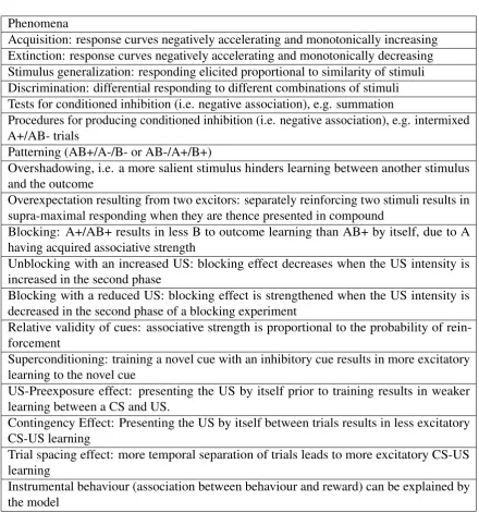
Phenomena

Acquisition: response curves negatively accelerating and monotonically increasing Extinction: response curves negatively accelerating and monotonically decreasing Stimulus generalization: responding elicited proportional to similarity of stimuli Discrimination: differential responding to different combinations of stimuli Tests for conditioned inhibition (i.e. negative association), e.g. summation

Procedures for producing conditioned inhibition (i.e. negative association), e.g. intermixed A+/AB- trials

Patterning (AB+/A-/B- or AB-/A+/B+)

Overshadowing, i.e. a more salient stimulus hinders learning between another stimulus and the outcome

Overexpectation resulting from two excitors: separately reinforcing two stimuli results in supra-maximal responding when they are thence presented in compound

Blocking: A+/AB+ results in less B to outcome learning than AB+ by itself, due to A having acquired associative strength

Unblocking with an increased US: blocking effect decreases when the US intensity is increased in the second phase

Blocking with a reduced US: blocking effect is strengthened when the US intensity is decreased in the second phase of a blocking experiment

Relative validity of cues: associative strength is proportional to the probability of rein-forcement

Superconditioning: training a novel cue with an inhibitory cue results in more excitatory learning to the novel cue

US-Preexposure effect: presenting the US by itself prior to training results in weaker learning between a CS and US.

Contingency Effect: Presenting the US by itself between trials results in less excitatory CS-US learning

Trial spacing effect: more temporal separation of trials leads to more excitatory CS-US learning

[image:42.595.86.527.106.578.2]

Instrumental behaviour (association between behaviour and reward) can be explained by the model

(43)

Phenomena

Spontaneous recovery: responding can resume after extensive extinction training

External disinhibition: presenting a salient yet novel cue before an extinguished cue can produce resumed responding

Reminder-induced recovery from extinction: presenting cues from previous training can produce resumed responding in an extinguished cue

Facilitated and retarded reacquisition after extinction: learning after an extinction treatment can occur at a different pace than before extinction training

Presenting a conditioned inhibitor by itself does extinguish its negative association Presenting a novel non-reinforced cue with a conditioned inhibitor does not lead to the former acquiring excitatory strength

Non-exclusiveness of conditioned excitation and conditioned inhibition: evidence suggests a cue can be both excitatory and inhibitory toward the same cue depending on the temporal relation between cues

Dependence of negative summation on the degree to which the transfer excitor is excitatory: a conditioned inhibitor can increase responding if the cue it is paired with was previously reinforced with a less intense reward than the one the conditioned inhibitor was paired with CS pre-exposure effect / Latent inhibition: presenting a CS by itself attenuates subsequent CS-US learning

Potentiation: presenting a salient CS with a less salient CS can sometimes produce more excitatory learning in the less salient CS, contradicting overshadowing

Second-order conditioning: pairing a cue A with an outcome, then cue B with cue A, results in cue B producing responding

Cue-to-consequence effects: CSs and USs from congruent sensory modalities are preferen-tially associated, e.g. flavours and gastric upset

Dependence of asymptotic responding on CS intensity: more intense CSs produce higher asymptotic responding

Learned irrelevance: uncorrelated CS-US presentations attenuate subsequent correlated CS-US learning with the same cues

One-trial overshadowing: overshadowing can occur within the first trial of training Overshadowing, blocking, and the US-preexposure effect are reversible.

Extinguishing the context can weaken the inhibitory strength of a conditioned inhibitor Superconditioning is sometimes not observed

Training cues A and B independently as excitors and then presenting them with novel cue X does not seem to make X a conditioned inhibitor as predicted

Large numbers of compound trials can eliminate overshadowing and blocking deficits Unblocking can be produced by omission of a second, expected US

Presenting a blocked CS without its blocking associate CS still leads to less excitatory learning than expected

A less salient CS is sometimes unable to block a more salient CS

(44)

Rescorla-Wagner and the Summation Assumption

When two or more stimuli are presented together, this presentation is termed acompound stim-ulus. Elemental models, which support strict summation, claim that an animal’s response to a compound stimulus will be equal to the sum of the responses, which each individual stimulus would have elicited when presented alone. This response is assumed to reflect the associative strength between the individual stimuli and the outcome. Thus, for instance when two stimuli (A& B) are individually reinforced and come to elicit respectively aCR_A andCR_B, their presentation together should elicit a CR of the magnitudeCR_A+CR_B. Other interpretations however violate the summation rule, and are supported by experimental evidence in many cases (Razran, 1939). They allow for the associative strength of a compound to be higher or lower than the direct summation of its constituent stimuli. This implies that additional information is encoded by the whole configuration of stimuli, distinct from their components.

Configuralmodels of learning posit that strict summation of associative strengths does not occur, and in fact animals represent compound stimuli through compound nodes with their own associative strengths. Thus the compound AB has an independent associative strength towards the outcome compared to its constituent stimuli, A and B. Existing elemental models lacked this representational feature and therefore needed a method to render non-linear discriminations. The introduction ofconfigural cues(Wagner and Rescorla, 1972) allowed the RW model to account for the failure of summation to materialize in certain compound trials, thereby retaining the structure of an elemental model while explaining the ability of animals to solve non-linear discriminations such as negative patterning (Rescorla et al., 1985) and biconditional discriminations (Rescorla, 1972; Saavedra, 1975). Negative patterning consists of nonreinforced stimulus compound trials being intermixed with reinforced pre-sentations of the individual stimuli. Biconditional discrimination is a procedure of the form

(45)

occur-rence of reinforcement. Thus the non-linear discrimination can only be solved by attending to the whole compound. These discriminations could not be resolved under the previous elemental frameworks1. Configural cues are assumed to emerge when a compound of two or more stimuli is presented (i.e. their stimuli representations are active concurrently). This cue acts as a stimulus in the learning process, and competes with other present stimuli. Take for example the case of negative patterning with intermixed A+/B+/AB- trials. The animal will learn to withhold its response during the presentation of the AB compound, as the configu-ral cueCemerging from this configuration undergoes inhibitory conditioning towards the US.

The RW model not only accounts for experimentally confirmed effects, but its formu-lation implied the existence of learning effects not predicted by earlier models or assumed to exist by pre-existing theory. Though the RW model has been successful in this regard (Miller et al., 1995), a summed error term is not the only means of predicting cue-competition results. Models relying on CS-US specific ’local’, non-competitive error-terms are capable of accounting for some of these effects by assuming other processes of competition, for instance on attentional competition between the predictors, as postulated by Nicholas Mackintosh (Mackintosh, 1975). Alternatively, the comparator hypothesis model (Miller and Matzel, 1988; Miller and Witnauer, 2016) explains cue-competition results as a retrieval effect. It assumes that when a previously reinforced CS is presented (the target), it re-activates both representations of other CSs paired with the US and the US representation itself. The re-sponse elicited by the target CS is then proportional to the degree to which it predicts the US relative to the associative strength of these comparator CSs. Hence cue-competition arises from the interference of other CS-US associations upon the target-US association (Figure 1.2).

(46)

[image:46.595.109.517.120.337.2]

Fig. 1.2The comparator hypothesis of Miller & Matzel (1988) postulates that the presentation of a CS invokes both a direct US representation, and an indirect activation of the US representation through comparators. These two pathways compete with one another to determine the net CR produced by the CS.

Temporal Difference learning

(47)

few erroneous predictions, such as that a co-occurring CS and US should become highly inhibitory towards one another. Flaws of the SB model are rectified in the Temporal Dif-ference (TD) model (Sutton and Barto, 1987) through the variations in the CS signal to the US node being dissociated from the US signal itself, and through the introduction of a time-discountγ to signal the uncertainty of future predictions. The TD model uniquely

predicts that learning is being driven by the need of the animal to minimise a time-discounted aggregate expectation of future reinforcement. At each time-step, the components of a given CS produce a prediction for the moment-by-moment change in US activation at the next time-step, termed the temporal difference. The difference between this prediction and the actual US activation level results in an error-term (similar to that in the RW model), the prediction error, for that time-step. The equation for calculating this error is as follows:

δt = (λt−(

_∑

i

xt_i−1V_it−γ

_∑

i

xt_iV_it)) (1.4) Hereλt is the US activation at timet,xt_i is the activation of a given CS, andVi is the

strength of the associative connection between CSiand the US. The term

_∑

xt_i−1V_it denotes the prediction for the US produced through the summation of associative activations of the US (using current associative links, but CS activation levels from the previous time-step), and the termγ

_∑

xt_iV_itis the equivalent for the current time-step. The current time-step prediction

is multiplied by the mentioned discount parameterγ to reflect that the future is always slightly

(48)

The error-term is used to adjust associative links between stimuli according to the equa-tion:

V_it =V_it−1+α δtxt_iet_i (1.5)

Here 0≤α ≤1 is the salience of the CS, and 0≤et_i≤1 is an eligibility trace of stimulus

i, which modulates the amount of learning a stimulus should receive based on the distance of the stimulus’ activation from that of the US. Eligibility traces can either accumulate to values higher than 1 over the duration of a stimulus, or build towards a value of 1 and then continuously undergo replacement by a value of 12. The equation for the latter, the

replacementeligibility trace, is:

e_it=min(1,ρ γe_it−1+xt_i−1) (1.6)

The trace therefore is set to and kept at 1 when a stimulus is active, and decays according to (0≤ρ≤1)·(0≤γ ≤1)every time-step when it is not active. This results in stimuli

receiving less reinforcement if there is a large gap between when they are active and when the US occurs.

The error-term can produce excitatory or inhibitory learning depending on whether the change in associative strength,∆V_it, is respectively positive or negative. Therefore, the speed

of learning between the CS and the US is inversely proportional to the certainty with which the animal can predict the occurrence of the US. This means that when the error of predicting

(49)

the US is reduced to zero, learning reaches an asymptote and effectively stops.

(50)

[image:50.595.91.511.120.372.2]

Fig. 1.3Simulation of the TD model using the TD simulator (Gray, J., Alonso, E., Mondragón, E., and Fernández, 2012). Displayed is the result of simulating acquisition for a reinforced serial compoundA→B→+(Group SC) compared toA→+(Group Ctrl). Group SC displays higher-order conditioning.

(51)

they are presented in succession. Steady evidence has mounted that predictions errors akin to the TD error are correlated to mid-brain dopamine function (Ludvig et al., 2011; Montague et al., 1996; Niv, 2009; Niv et al., 2012; Schultz, 2004, 2006, 2010; Schultz et al., 1997), specifically with increased dopaminergic activity corresponding to positive prediction errors, and lulls in dopaminergic activity corresponding to negative prediction errors. Furthermore, its efficacy in the domain of machine learning has been strengthened both due to its proven performance in practice, as well as mathematical analysis guaranteeing strong convergence properties toward an optimal policy (Sutton and Barto, 1998).

(52)

Elemental vs. Configural models: the nature of the stimulus

representa-tion

Causal relations in the world are mostly more complex than the linear CS-US relationship learned in a standard acquisition protocol, and thus non-linear conditional probabilities seem more appropriate to model them. That is, the probability of an outcome happening when multiple preceding events have occurred is not always equal to the product of the conditional probabilities of this outcome occurring given only one of the preceding events. Learning models therefore must in some manner involve processes of approximating these condition-ality relations, such as those seen in non-linear discrimination learning. Exactly how such causal connections are approximated is highly dependent upon how the stimuli themselves are represented by a model. Two benchmarks of non-linear discriminatory performance of a model have been the aforementioned negative patterning and biconditional discriminations. The difficulty, and hence importance, of negative patterning lies in the simple breakdown of linearity on the compound trials. That is, the animal must learn to withhold responding on trials when two cues, which individual predict the outcome, are presented. Biconditional discriminations involve yet more complex non-linearity. Four cues are presented in pairs, as the individual cues offer no information for solving the discrimination.

(53)

(54)

REM model

Such evidence of linearity of response summation being broken, prompted the conception of the replaced elements model (REM) (Wagner, 2003), which manoeuvred around this difficulty by a process whereby some elements of a stimulus are added (configural elements), and some are removed (unique elements), when the cue is presented in a compound. These added and replaced elements are consistent throughout presentations. The added elements correspond to elements representing context-dependent features of the stimulus (i.e. denoting conjunction with another cue), while the replaced elements are assumed to represent features of the cue that are uniquely present when the cue is presented alone. These statistically independent replacement rules are captured by the following relation:

P_A(A∪Comp.) =

_∏

K∈Comp.

(1−r_K) =

_∏

K∈Comp.

s_K (1.7) HereP_Adenotes the proportion of elements of stimulusAthat are sampled both whenA

is presented in isolation and when compound stimulus Comp. is presented. The similarity measure 1−rK orsK, denotes the quantity of elements that are sampled on bothAandAK

trials. Hence, the overall proportion of elements sampled on bothAand Comp. trials is the direct product of these binary relations.

(55)

[image:55.595.79.505.298.558.2]

of r upon the quantity of responding elicited by a CS compound ABafter A and B have been conditioned to an asymptotic level in isolation. Figure 1.4, r=0.0 leads to perfect summation of the strengths of A and B, whiler=1.0 leads to no responding, due to all the elements being replaced. Thus, by assuming that different modalities of stimuli undergo different replacement rates depending on their similarity, consistent with psychophysical theory (Glautier et al., 2010), the model can explain why summation seems to depend on the types of stimuli used (Wagner, 2003).

Fig. 1.4Simulation of the REM model using the REM simulator (Ghorashi, A., Mondragón, E. and Alonso, 2017). Results of the conceptual design 20A+/20B+ (random) followed by test trials for compound AB, withr=0 andr=1.

(56)

(57)

[image:57.595.123.465.109.359.2]

Fig. 1.51) An elemental connectionist structure. CSs are directly associated with the occurrence of the US. 2) A configural connectionist structure. CSs activate a configural representation, which in return enters into association with the US.

Pearce model

An alternative account to the elemental approach is supplied by the model of Pearce (Pearce, 1987), which in contrast presumes that nodes representing individual stimuli connect to an additional configural node representing their aggregation (as depicted in segment 2 of Figure 1.5). This node in return forms associations with the outcome.

The learning rule of the model hence involves calculating links between these configural nodes, and utilizes the following link-update equation:

∆Vi=β[λ−(Vi+

∑

i,j

(58)

HereViis the associative strength,β is the US salience,λ is the US asymptote,Si,jis the

similarity between stimuliiand j, and the sum ranges over all pairs of CSs. The similarity measure in return is calculated according to:

Si,j=

Nci N_t_i

Ncj

N_t_j (1.9)

Here,NciandNcj represent the number of elements respectively of cuesiand j, which

are common toiand j, andNtiandNtj are the total number of elements of the two cues.

(59)

[image:59.595.83.499.361.608.2]

(overshadowing). Yet it has been found that overshadowing produces a larger deficit in responding than external inhibition (Brandon et al., 2000). Finally, it has been found that familiarity with the constituent stimuli of a discrimination can facilitate the learning of the discrimination (Hall, 1991; Mondragón and Hall, 2002). This phenomenon of perceptual learning seems to suggest that the animal’s perception of the similarity of two stimuli is learned rather than given a priori as through the Pearce model’s similarity index. Hence, some form of attentional or learning-based process seems to be necessary to dichotomize unique and redundant elements of stimuli when they are pre-exposed together, such as elements shared by the pre-exposed stimuli losing associability.

(60)

Harris model

(61)

[image:61.595.124.464.111.356.2]

Fig. 1.7The fixed-capacity attentional buffer of the Harris (2006) model. Elements compete to enter the buffer, with those with a higher weight doing so more readily. The buffer increases the persistence of their activity. The number of US elements inside and outside the buffer determines the overall direction of learning (excitatory or inhibitory).

The entry to the buffer, as mentioned, is regulated by the weightωiof stimuli, such that:

∑

i

ωi≤ buffer capacity (1.10)

The actual entry of a given element is specified as occurring in proportion to∆ωi, which

is the difference between the intrinsic self-weight of a stimulus, and the prediction for it by other stimuli. Since this term acts as a prediction error, it is used in the associative strength update equation of the model:

∆Vx,y=



 

ωx·βy·2∆ωy if∆ωx>t

(62)

The response elicited by a stimulusAis thence calculated using the dot product over its elements:

R(A) =

_∑

i

ωAi·VAi (1.12)

(63)

the attentional buffer remains to be validated by empirical data. Further, many of the unique predictions of the model could be explained also for instance by the simpler assumption of the salience of a cue directly influencing the strength of its activation.

(64)

Attention and stimulus Pre-exposure: CS processing

As the Harris model assumes that any excitatory link from one stimulus to another induces activation in the recipient stimulus, it can explain various pre-exposure and habituation effects as well. In effect, the associability of a cue, all else being equal, is therefore directly proportional to its novelty. In addition, the model’s prediction that the effective associability of stimuli decreases in relation to how many further stimuli are active has been experimentally validated (Lachnit et al., 2008). This sets it in opposition to other paradigms of selective attention.

Mackintosh model

For instance, the Mackintosh model assumes that animals attend to cues that are relatively better predictors of outcomes than other cues (Mackintosh, 1975). It models the attention to a cue,αi, as changing in proportion to the relative predictiveness of the cue (in relation to

other cues) for the outcome. This is modelled through the equations that follow. The weight update rule is a ’local’, non-competitive one, similar to the Hull rule:

∆Vi=αi(λ−Vi) (1.13)

Unlike in the RW model, the cue-competition occurs through changes in the associability

αi. Theαiof a CS rises if|zλ−xiVi|<|zλ−VT|, whereVT is the total associative strength

of all other cues,zis the US presence, andλ is the US asymptote. This magnitude of change

is postulated to be in proportion to|zλ−xiVi| − |zλ−VT|. The implication is that selective

(65)

(66)

Pearce-Hall model

Conversely , the effect of Hall-Pearce negative transfer is easily accounted for by the Pearce and Hall (PH) model (Pearce and Hall, 1980), which postulates that attention rises when the outcome is uncertain, an assumption formalized in the following alpha update rule:

α_it=|zλt−1−

_∑

j

x_jVt_j−1| (1.14) whereα is once again the associability,zthe US presence,λ is the asymptote of learning,

andt represents trials.

Excitatory learning in the model is calculated using:

∆V_i+=α_itSizλ (1.15)

And inhibitory learning is calculated through:

∆V_i− =α_itSi(

∑

xiVi−zλ) (1.16)

In both equationsS_iis the salience of the US.

(67)

(68)

[image:68.595.137.468.266.462.2]

the cue. As such, the Le Pelley model can explain phenomena that have proven difficult for either model in isolation. It predicts for instance Hall-Pearce negative transfer as well as the learned irrelevance effect simultaneously. It however introduces further complexity as the two rules can often cancel the influence of one another . Thus, it is also difficult to isolate their respective effects empirically.

Fig. 1.8Simulation of the Pearce-Hall model using the Pearce-Hall Model Simulator (Grikietis, R., Mondragón, E., and Alonso, 2016). Alpha value of cue A in a simulation of 100A+/100A- is displayed.

SLGK model, Hall-Rodriguez model

(69)

US unit. These configural units have non-modifiable random incoming connections from all CS representations, and their connection to the outcome is modified through a delta rule. Their associability or associative rate is taken to be very low initially, however if the US novelty remains high during training (i.e. the animal is unable to learn a given contingency), then the associability of the configural units rises. It therefore accounts for the difficulty of animals to solve non-linear discriminations. This mechanism of detecting, through a persistent outcome error, when a purely linear approach has failed offers a robust approach for introducing non-linearity into models of conditioning while pre-empting a combinatorial explosion. It can be utilized to change the associability of other representational elements besides configural cues (e.g. common elements) to reflect when the animal cannot solve a learning problem.

(70)

[image:70.595.141.474.398.497.2]

interferes with the response elicited by the CS-US link formed in the subsequent acquisition training (Figure 1.9). This latter mechanism bears a similarity to the explanation offered by the comparator model, which similarly stresses processing during retrieval. Nevertheless, the neutral-learning based account of SLGK, SOP and McLaren-Mackintosh seems to hold a categorical advantage in explaining latent inhibition, as they do not need to assume such a no-US representation or the existence of an extant associative link to it. Hence they avoid predicting inhibitory properties of the pre-exposed CS towards the US, which have not been found in summation tests (Rescorla, 1971a). Further, the assumption of a no-US representa-tion implies a generalizarepresenta-tion of inhibirepresenta-tion to all reinforcers. However, CS-US learning has been shown to be highly US specific, for instance through reinforcer de-valuation effects (Colwill and Motzkin, 1994).

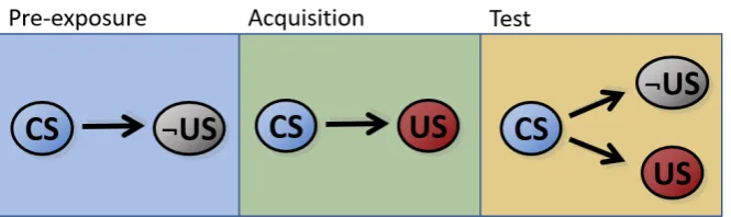
Fig. 1.9 (Hall and Rodriguez, 2010) postulates that pre-exposure induces the formation of aCS− ¬U S

link, that subsequently interferes with the CS-US link formed during acquisition.

(71)

(72)

Non-reinforced and Mediated Learning : neutral stimulus associations.

(73)

compared to the first phase of learning, whereas in the RR treatment the excitatory strength of B increases. That is, strengthening the association between one of the elements of the compound and the outcome, results in a reduction in strength of the concomitant stimulus and the outcome, whereas lowering it, raises the associative strength of its associated stimulus. In a forward and backward sensory preconditioning procedure either a simultaneous AB or serialB→A(FSP) or serialA→B(BSP) nonreinforced stimulus compound is first presented. In a second phase, A is reinforced. Subsequent test trials show that B, which has never been paired with the outcome, has nevertheless gained associative strength. Thus, an absent cue B undergoes a change in its associative strength as a consequence of the reinforcement treatment given to its associated cue.

One possible explanatory mechanism for these phenomena relies on the idea of mediated conditioning: During conditioning to A, an associative activation of stimulus B linked to A during the initial compound training is produced. This associatively activated representation of B thereupon strengthens or modulates associative connections between itself and other active stimuli. Of note is that the learning between the absent cue and the present outcome in SPC and BB proceeds in opposite directions, an apparent contradiction. Hence, though SPC can be explained as a mediated conditioning effect, BB cannot. Therefore, a robust explanation of mediated learning must take into account the prior learning taking place in SPC and BB.

Mediated learning has been conceptualized as a type of propositional reasoning process (Mitchell et al., 2009). As such, it can be understood through Bayes’ rule, which ties the conditional probability of one event E1 given another E2 (that isP(E₁|E2)) as changing

A Double-Error Correction Computational Model of Learning

City, University of London Institutional Repository

Citation:

This is the accepted version of the paper.

This version of the publication may differ from the final published

version.

Permanent repository link:

Link to published version:

Copyright and reuse: City Research Online aims to make research

outputs of City, University of London available to a wider audience.

Copyright and Moral Rights remain with the author(s) and/or copyright

holders. URLs from City Research Online may be freely distributed and

linked to.

A Double-Error Correction

Computational Model of Learning

Niklas H. B. Kokkola

Supervisor: Dr. Eduardo Alonso

First Supervisor

Dr. Chris Child

Second Supervisor

Dr. Esther Mondragón

External Supervisor

This dissertation is submitted for the degree of

Doctor of Philosophy

City, University of London

Department of Computer Science

Table of contents

List of figures

List of tables

Contributions

Declaration

Abstract

Chapter 1

Literature Review and Methodology

1.1

Motivation

1.2

Contributions

1.3

Overview of Work

1.4

Summary of the Model

1.5

Literature Review

List of abbreviations for Chapters 1-3

Associative Learning

∑

∑

∑

∑

∑

∑

Elemental vs. Configural models: the nature of the stimulus

representa-tion

∏

∏

∑

∑

∑

Attention and stimulus Pre-exposure: CS processing

∑

∑

Non-reinforced and Mediated Learning : neutral stimulus associations.

_∑

_∑

_∑

_∑

_∏

_∏

_∑

_∑