Negative emissions—Part 2: Costs, potentials and side effects

TOPICAL REVIEW • OPEN ACCESS

Negative emissions—Part 2: Costs, potentials and

side effects

To cite this article: Sabine Fuss et al 2018 Environ. Res. Lett. 13 063002

View the article online for updates and enhancements.

Related content

Negative emissions—Part 1: Research landscape and synthesis

Jan C Minx, William F Lamb, Max W Callaghan et al.

-Negative emissions—Part 3: Innovation and upscaling

Gregory F Nemet, Max W Callaghan, Felix Creutzig et al.

-2 °C and SDGs: united they stand, divided they fall?

Christoph von Stechow, Jan C Minx, Keywan Riahi et al.

-Recent citations

Targeted policies can compensate most of the increased sustainability risks in 1.5 °C mitigation scenarios

Christoph Bertram et al

-Negative emissions—Part 3: Innovation and upscaling

Gregory F Nemet et al

-Negative emissions—Part 1: Research landscape and synthesis

Jan C Minx et al

TOPICAL REVIEW

Negative emissions—Part 2: Costs, potentials and side

effects

Sabine Fuss1,11 _{, William F Lamb}1 _{, Max W Callaghan}1,2_{, J´er ˆome Hilaire}1,5 _{, Felix Creutzig}1,3_{, Thorben}

Amann4 _{, Tim Beringer}1_{, Wagner de Oliveira Garcia}4 _{, Jens Hartmann}4 _{, Tarun Khanna}1_{, Gunnar}

Luderer5_{, Gregory F Nemet}6 _{, Joeri Rogelj}7,8 _{, Pete Smith}9 _{, Jos´e Luis Vicente Vicente}1_{, Jennifer Wilcox}10_,

Maria del Mar Zamora Dominguez1_{and Jan C Minx}1,2

1 _{Mercator Research Institute on Global Commons and Climate Change, Torgauer Straße 12–15, EUREF Campus #19, 10829 Berlin,}

Germany

2 _{School of Earth and Environment, University of Leeds, Leeds LS2 9JT, United Kingdom} 3 _{Technische Universit¨at Berlin, Straße des 17. Juni 135, 10623 Berlin, Germany} 4 _{Universit¨at Hamburg, Bundesstraße 55, 20146 Hamburg, Germany} 5 _{Potsdam Institute for Climate Impact Research, D-14473 Potsdam, Germany}

6 _{La Follette School of Public Affairs, University of Wisconsin–Madison, 1225 Observatory Drive, Madison, WI 53706, United States of}

America

7 _{ENE Program, International Institute for Applied Systems Analysis (IIASA), Laxenburg, Austria} 8 _{Institute for Atmospheric and Climate Science, ETH Zurich, Zurich, Switzerland}

9 _{Institute of Biological and Environmental Sciences, University of Aberdeen, 23 St Machar Drive, Aberdeen, AB24 3UU, Scotland,}

United Kingdom

10 _{Department of Chemical and Biological Engineering, Colorado School of Mines, Golden, CO, United States of America} 11 _{Author to whom any correspondence should be addressed.}

OPEN ACCESS

RECEIVED

20 October 2017

REVISED

30 March 2018

ACCEPTED FOR PUBLICATION

20 April 2018

PUBLISHED

22 May 2018

Original content from this work may be used under the terms of the Creative Commons Attribution 3.0 licence.

Any further distribution of this work must maintain attribution to the author(s) and the title of the work, journal citation and DOI.

E-mail:[email protected]

Keywords:climate change mitigation, negative emission technologies, carbon dioxide removal, scenarios

Supplementary material for this article is availableonline

Abstract

The most recent IPCC assessment has shown an important role for negative emissions technologies

(NETs) in limiting global warming to 2

C cost-effectively. However, a bottom-up, systematic,

reproducible, and transparent literature assessment of the different options to remove CO

from the

atmosphere is currently missing. In part 1 of this three-part review on NETs, we assemble a

comprehensive set of the relevant literature so far published, focusing on seven technologies:

bioenergy with carbon capture and storage (BECCS), afforestation and reforestation, direct air carbon

capture and storage (DACCS), enhanced weathering, ocean fertilisation, biochar, and soil carbon

sequestration. In this part, part 2 of the review, we present estimates of costs, potentials, and

side-effects for these technologies, and qualify them with the authors

assessment. Part 3 reviews the

innovation and scaling challenges that must be addressed to realise NETs deployment as a viable

climate mitigation strategy. Based on a systematic review of the literature, our best estimates for

sustainable global NET potentials in 2050 are 0.5–3.6 GtCO

yr

for afforestation and reforestation,

0.5–5 GtCO

yr

for BECCS, 0.5–2 GtCO

yr

for biochar, 2–4 GtCO

yr

for enhanced

weathering, 0.5–5 GtCO

yr

for DACCS, and up to 5 GtCO

yr

for soil carbon sequestration.

Costs vary widely across the technologies, as do their permanency and cumulative potentials beyond

2050. It is unlikely that a single NET will be able to sustainably meet the rates of carbon uptake

described in integrated assessment pathways consistent with 1.5

C of global warming.

1. Introduction

The Paris goal of holding global warming‘well below 2◦C’and to‘pursue efforts’to limit it to 1.5◦C imply

a starkly limited remaining CO₂budget (IPCC2013,

2014b, Rogeljet al2016). Considering the lack of deep,

need to play a progressively more important role in cli-mate stabilization strategies (Rogeljet al2015a, Luderer

et al2013).

Studies applying global Integrated Assessment Models (IAMs) have highlighted the strategic and long-term importance of CDR for cost-effectively lim-iting global warming to 2◦C (Kriegleret al2014), the key technology being Bioenergy with Carbon Capture and Storage12 (BECCS) (Fusset al2014, Clarkeet al 2014)13_{. Rogeljet al(2018) analyse the most recent and}

comprehensive set of 1.5◦C scenarios, which remove about 15 GtCO₂yr−1(median, 3–31 full range) by 2100 through BECCS. This corresponds to 175 (median, 54–404 full range) EJ yr−1 of bioenergy. Such large amounts of bioenergy can however imply trade-offs with other land-based policy goals such as biodiver-sity conservation and food production (e.g. Kraxner

et al(2013), see Creutzig (2016) for a discussion of the associated views). Recently, afforestation and refor-estation have been added to many of the IAMs, which explicitly model the land use sector or are coupled to large-scale, geographically explicit land use models (e.g. Humpen¨oderet al2014, Calvinet al2014).

However, in order to perform a high-quality inte-grated assessment of NETs, a characterization of the different options is needed. A variety of reviews on NET technologies have taken on this task over the

years (Smith et al 2016a, National Academy of

Sci-ences2015, Caldecottet al2015, Lenton2014,2010,

McGlashanet al 2012, McLaren2012, Vaughan and

Lenton 2011, The Royal Society 2009). From the

approximately 3000 articles on NET technologies and measures identified by Minxet al(2017), more than 200 are classified as review articles. However, the available assessments have three shortcomings: first, they insuf-ficiently bridge the divide between strategic evidence from long-term climate change mitigation models and the technological and institutional bottom-up evidence from the engineering and social science disciplines

(Minx et al 2018). Second, the assessment of the

entire NETs portfolio has been very fragmented so far, with only one publication assessing a full set of options (Friends of the Earth2011), and other impor-tant efforts missing out technologies such as biochar and soil carbon sequestration (National Academy of Sciences2015). Third, none of the available NETs and geoengineering assessments provide a systematic, com-prehensive and transparent analysis rooted in a formal review methodology.

As in the two companion papers to this piece (Nemet et al 2018, Minx et al 2018), our review is

12 _{Although the term storage might imply accumulation for future}

use, we use it here interchangeably with the term‘sequestration’in accordance with the literature reviewed.

13 _{Notable exceptions are Marcucciet al(2017), Chen and Tavoni} (2013) and Strefleret al(2018b) for DACCS and Strefleret al(2018a) for terrestrial enhanced weathering. Strefleret al(2018b) combined three NETs (AR, BECCS and DACCS) for the first time.

formalized according to standard systematic review procedures (such as those more frequently employed in the medical and social sciences): (1) a search query is defined for each NET to transparently identify the relevant literature; (2) studies are then individ-ually excluded according to pre-defined eligibility criteria; (3) qualitative and quantitative evidence is extracted and synthesized from the final document set (see the supporting information (SI) available

atstacks.iop.org/ERL/13/063002/mmediafor the full

protocol). Such a procedure is necessary to ensure reproducibility, avoid systematic omissions or biases in literature selection and to deal with a rapidly expanding base of knowledge (Minxet al2017).

This paper is divided into two main parts. The first section proceeds with a review of low-stabilization scenarios from the IAM literature, examining the role of negative emissions in the mitigation portfo-lio and the magnitudes of CO₂that would be removed from the atmosphere. The second part comprises our bottom-up review of individual NETs technologies and options, with a particular focus on magnitudes, costs and side-effects—both negative (e.g. competi-tion for land, biodiversity loss or increased ocean acidification) and positive (e.g. health benefits from reduced air pollution, reduced ocean acidification, energy access—particularly off-grid). While the sce-nario literature in the past has mostly incorporated negative emissions in the form of BECCS and afforesta-tion and reforestaafforesta-tion, we here consider a larger range of negative emissions options, including biochar, enhanced weathering, ocean fertilization, direct air car-bon capture and storage, soil carcar-bon sequestration and some further options with smaller literature bases.

2. Scenario evidence on the role of negative

emissions

The IPCC’s Fifth Assessment report highlighted a

potentially important role for NETs in keeping global temperature rise below 2◦C with a probability greater

than 66% (IPCC 2014a, Clarke et al 2014). More

recently the ambition of the Paris Agreement not

only to keep warming well below 2◦C, but to

pur-sue further efforts to limit warming to below 1.5◦C

(UNFCCC2015) has pushed NETs into the spotlight

of discussions on viable mitigation pathways (Hulme

2016, Peters2016, Rogeljet al2015a, Hallegatteet al 2016, Ludereret al2013). A series of high level com-mentaries and recent articles further elevated the issue and emphasized the controversial nature of NETs deployments featured in long-term mitigation

sce-narios (Geden 2015, Anderson 2015, Anderson and

Peters2016, Gasseret al2015, Peters and Geden2017,

Lomax et al 2015, Williamson 2016, Parson 2017,

Field and Mach2017). We engage with this

In this section we review publicly available data from multi-model inter comparison studies14_{in order}

to understand the role of NETs in climate change miti-gation (Riahiet al2015, Kriegleret al2015, GEA2012, Riahi et al 2017, van Vuuren et al 2017a, Kriegler

et al 2013b, 2016b). We supplement this data with further scenario evidence on the 1.5◦C limit (Lud-erer et al 2013, Rogelj et al 2015a, 2013a, 2013b,

2018). Hence the comprehensiveness and transparency of our review in this section is related to pooling the available data from recent studies. While many of the recent IAM scenarios include negative emissions, we only systematically review the literature that give sufficient importance to NETs, i.e. where NETs are mentioned in abstract, keywords or title. Importantly, the vast majority of mitigation scenarios considered here only features negative emissions via bioenergy with carbon capture and storage (BECCS). We inter-pret this evidence as a lower-bound estimate of negative emission potentials in these models, since the introduc-tion of addiintroduc-tional NETs seems to consistently increase

cumulative NETs deployment (Chen and Tavoni2013,

Humpen¨oderet al2014, Marcucciet al2017).

2.1. Understanding the role of negative emissions for achieving alternative long-term climate goals The carbon budget has been established in IPCC AR5 as a fundamental concept to understand human-induced (long-term) warming. It is defined as the cumulative amount of net CO₂emissions that can be released while still limiting warming with a specific minimum proba-bility to below a given temperature threshold (IPCC

2013, 2014b, Rogelj et al 2016). In principle, gross

CO₂ emissions can be larger than the carbon

bud-get as long as they are simultaneously compensated by negative emissions (figure1) (Kriegleret al2014, Riahi

et al 2015, Eom et al 2015, van Vuuren et al 2013,

van Vuuren and Riahi2011, van Vuurenet al 2007,

Azar et al2006,2010). Yet the geophysical limits of negative emissions are currently not well understood (Rogelj and Knutti2016), although they are starting to be explored more rigorously (Kelleret al2018). A recent study asserts that the carbon budgets associ-ated with the Paris Agreement temperature goals can

be revised upwards from AR5 estimates (Millaret al

2017). This discussion is still new and unresolved. In the absence of a broader body of evidence we maintain

the estimates from the IPCC AR5 (IPCC2014b).

Looking across the available scenario evidence, two major purposes of negative emissions in climate change mitigation can be identified: first, NETs are deployed in scenarios for biophysical reasons, because the carbon budget consistent with a given tempera-ture target is exceeded (van Vuuren et al2007, van Vuuren and Riahi2011, Clarkeet al2014). The‘ pay-back’ for this temporary exceedance is the required amount of cumulative net negative emissions, i.e. the total global net removal of carbon dioxide from the atmosphere towards the end of the 21st century when

NETs draw global emission levels below zero (Blan-ford et al2014, Kriegler et al2013a). Compensation of excess positive emissions by negative emissions can come with a penalty (or‘interest’), because the cooling from net negative anthropogenic emissions may only offset part of the warming from earlier positive emis-sions (Zickfeldet al2016). Second, negative emissions are deployed in scenarios for intersectoral compensa-tion, i.e. to offset residual emissions that are difficult to mitigate, such as transportation—especially emis-sions from aircraft—and industrial emisemis-sions (Rogelj

et al2015a), or non-CO₂GHGs from agriculture (Ger-naatet al2015). This occurs particularly in the second half of the 21st century when high carbon prices are realized in integrated assessment models. In figure2

this can be observed when the total removal of CO₂

by NETs—henceforth referred to as gross negative emissions—is much larger than cumulative net neg-ative emissions (Kriegleret al2013a, van Vuuren and Riahi2011, Kreyet al2014a, van Vuurenet al2013). It is important to note that in some scenarios NETs are predominantly deployed because they are econom-ically attractive (Azaret al 2006, Luckowet al 2010, Lemoineet al2012), while in others they are biophysi-cally required. For instance, some scenarios show that with immediate strengthening of climate policies it is still possible to limit warming to below 2◦C without NETs (Kriegleret al2014). However, further delay of action or the tighter 1.5◦C climate goal renders NETs indispensable in the currently available scenarios.

Figure3provides an overview of emission pathways for achieving alternative climate targets and the role of negative emissions therein (Panel A). Scenario evidence available on the 1.5◦C warming limit remains compar-atively limited. For IPCC AR5, evidence from only two models was available (Ludereret al2013, Rogeljet al

2015a,2013a,2013b). We complement these studies

with more recent 1.5◦C scenarios that span a variety of socio-economic conditions (Rogeljet al2018).

Temperature overshoot is a typical feature in avail-able 1.5◦C scenarios although the current scenario literature has not specifically focused on avoiding it15_.

All available scenarios hence show net negative cumu-lative emissions budgets for the second half of the 21st century (2050–2100) (Rogeljet al2015a,2018) or even

in the longer run until 2300 (Akimoto et al 2017).

14_{LIMITS (https://tntcat.iiasa.ac.at/LIMITSDB/), AMPERE} (https://tntcat.iiasa.ac.at/AMPEREDB/), RoSE ( www.rose-project.org/database) provide results for hundreds of scenar-ios from roughly a dozen of models in the absence of explicit information on NETs in the even larger IPCC scenario database (https://tntcat.iiasa.ac.at/AR5DB/). We also include the SSP scenar-ios (https://tntcat.iiasa.ac.at/SspDb/). A description of the models that produced the scenarios analysed in this section is available in the SI.

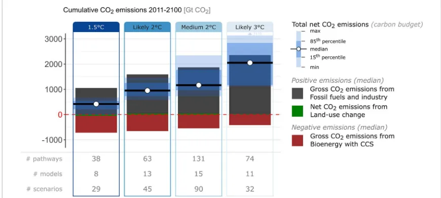
Figure 1.Positive and negative CO₂emission components for reaching alternative temperature goals. Basic descriptive statistics of the underlying data is provided under the bar plot; more detailed data is available in the SI. Values in the row labelled‘pathways’

indicate the number of available individual pathways. Those in the rows‘models’and‘scenarios’indicate the number of available individual models (see SI for model description) and scenarios. Important note: median values for gross negative CO₂emissions can be considerably lower when a larger ensemble of scenarios is considered, as can be seen in figure3. Yet not all emission categories were available from all modelling teams (e.g. gross positive emissions from fossil fuels and industry and net land-use change), so we had to take a smaller sample (see table S16 in SI). In the following paragraphs of this section on scenarios however, we focus on negative emissions and so we use the more complete dataset from figure3.

Box 1. Defining climate policy scenarios in terms of warming limits.

We analyze the role of negative emissions for keeping temperature rise below alternative warming thresholds—namely 1.5◦C, 2◦C and 3◦C. For this purpose we define scenarios in terms of a minimum probability (usually 66%; sometimes 50%) for temperature rise not to exceed a certain warming threshold (Rogeljet al2016), as conventionally done in the literature (Rogeljet al2015a, Ludereret al 2013, Rogeljet al2011, Clarkeet al2014):

∙1.5◦C scenarios: Scenarios with a probability greater than 50% of reverting warming below 1.5◦C by 2100.

∙Likely 2◦C scenarios: Scenarios that keep warming below 2◦C with a greater than 66% probability throughout the 21st century.

∙Medium 2◦C scenarios: Scenarios that keep warming below 2◦C with a greater than 50% probability throughout the 21st century. Most of the scenarios that meet this criterion introduce adequate climate policies after an initial delay (delayed action scenarios).

∙Likely 3◦C scenarios: Scenarios that keep warming below 3◦C with a greater than 66% probability throughout the 21st century. For most scenario studies the reduced-form carbon-cycle and climate model MAGICC was used in a probabilistic setup to determine implied warming levels (Meinshausenet al2011, Rogeljet al2012, Schaefferet al2015). While some of these scenario categories are more in line with the Paris Agreement long-term temperature goal, they do not represent a formal interpretation of the UNFCCC temperature goal.

All these 1.5◦C scenarios are fundamentally depen-dent on the global-scale availability of NETs (figure3). Scenarios that restrict16 _{the availability of NETs}

sub-stantially often result in model infeasibility (Luderer

et al2013). However, recent structured explorations of various socioeconomic contexts, the so-called Shared

Socioeconomic Pathways (SSPs) (Riahi et al 2017,

O’Neill et al 2017), have shown that NETs use

can be restricted to some degree in 1.5◦C

scenar-ios if specific socioeconomic conditions are met, such as low energy demand, sustainable consump-tion patterns and high crop yield improvements (SSP1) (Rogeljet al2018).

Transition pathways limiting climate change to 1.5◦C are consistently characterized by sharp

imme-diate reductions of net CO₂emissions (3%–7% yr−1

on average between 2030 and 2050, taking 2030 as a reference) that lead to a fully decarbonized world (net zero emissions globally) between 2046 and 2056

(15th and 85th percentiles), with a sustained period of annual net negative emissions17_{ranging between 1.3–}

29 GtCO₂yr−1 during the second half of the century. In general, NETs deployment throughout this period is large-scale in currently available scenarios. By 2050 NETs deployment is already between 5 GtCO₂yr−1and 15 GtCO₂yr−1in most scenarios. The associated scale-up of NETs between 2030 and 2050 therefore takes place much more swiftly than in most 2◦C scenarios,

removing an additional 0.1–0.8 GtCO₂every year on

average. Total NETs deployment across the 21st cen-tury is associated with a cumulative removal of carbon of 150–1180 GtCO₂.

16_{Typical restrictions imposed are the unavailability of CCS and a}

restriction of the annual bioenergy potential to 100 EJ (Kreyet al 2014b, Ludereret al2013, Clarkeet al2014).

17_{Please note that this analysis only considers gross negative}

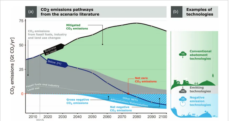
(a) (b)

Figure 2.The role of negative emissions in climate change mitigation. The graph juxtaposes emission reductions from conventional mitigation technologies (panel A) with the removal of carbon dioxide via negative emissions technologies (panel B) in an exemplary scenario consistent with a 66% chance of keeping warming below 2◦C relative to a baseline scenario. Global emission levels turn net negative towards (hatched blue area) the end of the century to compensate for earlier carbon budget overshoot. Cumulative gross negative emissions represented by the entire blue area. The exemplary scenarios‘business as usual’and‘below 2◦C’were constructed using data from the LIMITS database (https://tntcat.iiasa.ac.at/LIMITSDB/). They correspond to the RefPol and LIMITS-RefPol-450 scenarios produced with the MESSAGE model. Gross positive and negative CO₂emissions from land-use changes labelled as‘land use’(bottom grey shaded area) and‘afforestation/reforestation’(bottom blue shaded area) were inferred from net land-use changes emissions by using data in figure SI13 in Poppet al(2017). This manual edit was done to account for current afforestation and reforestation efforts and differentiate between negative emissions from land-use changes and other NETs.

Our ranges describe the statistics of an ensem-ble of opportunity, which has not been designed to span all possible outcomes in terms of NETs deployment. It mostly represents dynamics that are considered cost-effective by models in absence of particular societal preferences. The ranges thus repre-sent characteristics of the currently available literature. Additional research needs to confirm that these can also be interpreted as requirements in a more formal sense.

Compared to 1.5◦C scenarios, the literature on the

role of NETs in 2◦C scenarios is much more mature

and rooted in a series of inter-model comparison exer-cises (Riahiet al2015, Kriegleret al2013b, Kreyet al

2014b, Kriegler et al 2016b, 2016a, 2014, Fuss et al

2014, Tavoni and Socolow2013, Kriegleret al2013a,

van Vuurenet al2013). These have been summarized

in IPCC AR5 (Clarkeet al 2014). In 2◦C scenarios NETs are primarily deployed for limiting overshoot in atmospheric concentrations rather than tempera-tures (Riahi et al 2015, Blanford et al 2014, Tavoni and Socolow2013, van Vuurenet al2013). While this still leads to a significant reduction in the probabil-ity of reaching the long-term climate goal (Schaeffer

et al 2015, Riahi et al 2015, Eom et al 2015), tem-perature overshoot carries additional risks associated with higher levels of warming and the resulting impacts and climate feedbacks that could occur (van Vuuren

et al 2013, Solomon et al 2009, Friedlingstein et al 2006, Clarkeet al2014).

In general, 2◦C scenarios feature much more flex-ibility in NETs deployment, covering a wide range from zero to levels comparable with higher bound deployments in 1.5◦C scenarios. Hence, it is impor-tant to highlight that while many 2◦C scenarios deploy NETs at large scale, there are also scenarios that do not deploy NETs at all, or at very low levels (e.g. Eom et al 2015, Kriegler et al 2014, Luderer et al 2013, Riahiet al2015, Rogeljet al2013a)—an aspect that is often sidelined in discussions but is crucial for understanding the policy option space (Eden-hofer and Kowarsch2015, Minxet al2017). For 2◦C scenarios featuring NETs deployment, it also points towards a strong economic rationale within models, as towards the end of the 21st century NETs become economically attractive if a temporary overshoot of the CO₂budget is allowed, or if residual GHG emissions from other sectors are highly expensive to mitigate (Kriegleret al2013b, Kreyet al 2014a, Kriegleret al

2014).

In the 2◦C scenarios18_{with immediate}

implemen-tation of climate policy and no additional technological constraints, net CO₂emission reductions between 2030 and 2050 take place at an average rate of 1%–4%

per year (Riahi et al 2015). After 2080 more than

two thirds of these 2◦C scenarios have completed

the decarbonisation of the world economy, i.e. they

(a)

(b)

(c)

(d)

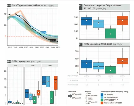
Figure 3.The role of negative emissions for achieving alternative long-term climate goals. Climate goals are indicated with blue shades. The more stringent the climate goal, the darker the blue colour. Net CO₂emissions are displayed in panel (a) (top-left). Ribbons indicate the 15th and 85th percentiles for each climate goal. The original RCPs and the SSP2–2.6 marker scenarios are provided for orientation purposes. The boxplots in panels (b)–(d) provide the same statistics. The range between the minimum and maximum values is indicated with a vertical solid line. The range between the 15th and 85th percentiles is indicated by a blue-filled rectangle. The median is shown with a solid horizontal line whereas the mean is indicated by a white point. NETs deployments in 2030, 2050 and 2100 are shown in panel (b). Cumulative gross negative CO₂emissions between 2011 and 2100 are shown in panel (c). Annually averaged gross negative CO₂emissions between 2030 and 2050 are displayed in panel (d). Descriptive statistics of the underlying data are provided under panel (d) and more detailed data is available in the SI. Statistical differences between figures1and3arise because a few modelling teams did not report all variables necessary to plot figure1(i.e. gross positive emissions from fossil fuel and industry, net land-use emissions). A description of the models is provided in the SI.

transition from net positive to net negative CO₂

emis-sions (Rogelj et al 2015b). While there are some

scenarios available without net negative emissions at the end of the century, most scenarios feature

consid-erable NETs deployment ranging from 5 GtCO₂yr−1

to 21 GtCO₂yr−1at the end of the 21st century. These annual deployment ranges are therefore not much lower than for 1.5◦C scenarios. In 2◦C scenarios with limited or no negative emissions (labelled with

‘limited bioenergy’or‘no CCS/BECCS’), decarboni-sation (including fossil fuel phase-out) occurs more rapidly than in the most cost-efficient 2◦C scenarios (full portfolio), but at a higher overall cost (Kriegler

et al2014, Kreyet al2014a, Riahiet al2015, Luderer

et al2014). For instance, Ludereret al(2013)—based on the REMIND model—show that mitigation costs defined as the ratio of discounted19 _{and aggregated}

19 _{Ludereret al(2013) applied a discount rate of 5% to both} con-sumption losses and GDP.

consumption losses over discounted and aggregated GDP increase from 1.4% to 1.9% if BECCS (as the only explicit NETs option in the model) is limited, and to 2.3% in the absence of BECCS in 2◦C scenarios. Lim-iting BECCS in 1.5◦C scenarios increases costs from 2.3%–4.1%, while the absence of BECCS makes the sce-narios infeasible. Similarly, multi-model results from EMF27 highlight the most significant cost mark-up for imposed technology constraints when CCS remains absent and bioenergy is limited to 100EJ (Kriegler

et al2014). One key reason for the larger cost mark-ups could be the constraints imposed on the NETs deploy-ment potentials in the scenarios. Klein et al (2014) show that the negative emissions value of biomass tends to dominate over its energy value in low stabilization scenarios.

(a) (c)

(d)

(b)

Figure 4.Negative emissions have a distinct role in 2◦C scenarios depending on the technological options and policy timing. Technological options and policy timing are indicated with various colours (dark blue for full technological portfolio, light blue for low energy intensity, green for limited biomass and no CCS/BECCS, and red for delay action until 2030). The cases full portfolio, low energy intensity and limited biomass or no CCS/BECCS assume climate action from 2010 onward. Net CO₂emissions are displayed in panel (a) (top-left). Ribbons indicate the 15th and 85th percentiles for each pathway category. The original RCP-2.6 (also called RCP-3PD) and the SSP2–2.6 marker scenarios are provided for orientation purposes. The boxplots in panels (b)–(d) provide the same statistics. The range between the minimum and maximum values is indicated with a vertical solid line. The range between the 15th and 85th percentiles is indicated by a blue-filled rectangle. The median is shown with a solid horizontal line whereas the mean is indicated by a white point. NETs deployments in 2030, 2050 and 2100 are shown in panel (b). Cumulative gross negative CO₂emissions between 2011 and 2100 are shown in panel (c). Annually averaged gross negative CO₂emissions between 2030 and 2050 are displayed in panel (d). Basic descriptive statistics of the underlying data are provided under panel (d), and more detailed data is available in the SI. 2◦C scenarios include both likely 2.0◦C and medium 2.0◦C scenarios. A description of the models is provided in the SI.

(Rogelj et al 2013b, Krey et al 2014a, Eom et

al 2015). In particular, gross cumulative negative

emissions deployment (290–760 GtCO₂) tends to be

lower in these scenarios driven by lower deployment rates (0–7 GtCO₂yr−1) and upscaling (0–0.3 of addi-tional GtCO₂yr−1) between 2030 and 2050. Further delay in adequate global climate action swiftly locks 2◦C pathways with NETs in, including delayed action until 2030 (as implied by current NDC ambitions). Like most 1.5◦C scenarios, these 2◦C pathways can no longer be achieved without any or even limited amounts of NETs (figure5) (Ludereret al2013, Riahiet al2015). Deployment and upscaling rates also increasingly mir-ror those seen in the available 1.5◦C scenarios.

The CO₂removal ranges presented in this review

are much wider than those reported in (Clarkeet al

2014) and (Rogeljet al2015a). The underlying scenar-ios are almost exclusively assuming middle-of-the-road and do not consider systematically socio-economic variations in future conditions. Here, such variations

are considered via the new shared socio-economic pathways (SSPs) (Riahiet al2017, O’Neillet al2017, Rogeljet al2018). One important insight from this new evidence is that the role and importance of NETs in cli-mate change mitigation scenarios depends crucially on socio-economic developments (Riahiet al2017, Bauer

et al2017, Poppet al2017, van Vuurenet al2017b, Rogeljet al2018). For optimistic storylines following a sustainability narrative (SSP1). NETs requirements can be substantially lower than in middle of the road scenarios (SSP2) (Riahiet al2017, Rogeljet al2018). Conversely, the dependence on NETs increases in sce-narios characterized by high energy demand and a strong preference for using fossil fuels (SSP5). For

instance, to keep global warming below 1.5◦C the

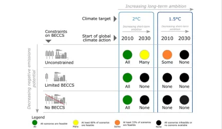
Figure 5.Model feasibility for different climate policy scenarios. Scenarios differ with respect to the climate policy ambition, the timing of climate policy and the assumptions of the available technology portfolio. All scenarios share the same exogenous socio-economic assumptions for GDP, population and energy demand.‘Many’means that less than 50% of the model runs were feasible whereas

‘some’means that less than 33% of the model runs were feasible. Data come from REMIND model runs (Ludereret al2013). 2◦C scenarios include both likely 2◦C and medium 2◦C scenarios.

(SSP3), or strong inequality within and between world regions (SSP4), would feature different NETs require-ments. Beyond discussions of how to organize climate and energy policies with regard to negative emissions (Peters and Geden2017), it is therefore also crucial to start a discussion on how the general development tra-jectory affecting consumption patterns, energy demand and international cooperation can be changed in light of its impact on NETs reliance to achieve stringent climate objectives.

While the vast majority of studies feature BECCS as the only explicit NET in the portfolio, a num-ber of studies examine the role other NETs, often in small portfolios of two NETs that include BECCS. These studies looked at afforestation and reforesta-tion (AR) (Humpen¨oderet al2014, Kreidenweiset al 2016, Tavoni et al 2007, Edmondset al 2013, Reilly

et al2012, Poppet al2017, Rose et al2012, Calvin

et al 2014), enhanced weathering (EW) and direct air carbon capture and storage (DACCS) (Marcucci

et al 2017, Chen and Tavoni 2013, Strefler et al

2018b). The IAM community is currently

investigat-ing the role of larger NETs portfolios includinvestigat-ing AR, BECCS, DACCS and EW.

The IAM literature on AR has now become sub-stantial. It shows an average cumulative potential for AR over the 21st century and across models

ranging from 200–860 GtCO₂ (Humpen¨oder et al

2014, Kreidenweis et al 2016, Rao and Riahi 2006, Calvinet al2014, Tavoni et al 2007, Edmondset al 2013, Reillyet al2012). The upper end of the range is computed by models that include endogenous

technological change (Humpen¨oderet al2014, Krei-denweis et al 2016, Edmonds et al 2013). Yet it is interesting to note that a model that does not consider this effect, but includes the impacts of climate change on crop yields, still reports estimates up to 650 GtCO₂

(Reilly et al 2012). The lower end of the range of

results is associated with modelling constraints (e.g. limits on bioenergy production or the availability of BECCS). Maximum annual deployments over the 21st

century range between 0.5–10 GtCO₂ (Humpen¨oder

et al2014, Poppet al2017, Reillyet al2012). A com-mon finding to all the selected studies is the low cost of implementing AR compared to that of other NETs. For instance, Strengerset al (2008) estimated that about 50% of the potential would be available at costs below 55 US$/tCO_2, while Humpen¨oder et al (2014) note that AR starts at carbon price as low as 6 US$/tCO₂. In terms of policy costs, AR can decrease the costs of mit-igating climate change by about US$3 trillion (Tavoni

et al2007).

the cumulative removal is large-scale, up to about 500 GtCO₂, and hence is associated with a sharp decline of atmospheric CO₂concentrations. Uncertainty sur-rounding the development and implementation costs of this technology currently remains a major barrier (see section3.3). Finally, Strefleret al(2018a) assess the techno-economic potential for land-based enhanced weathering at about 5 GtCO₂for both basalt and fos-terite. Adding it to the technology portfolio reduces the carbon price (Strefler et al2018a). Because EW does not compete with BECCS, this technology might be particularly valuable if other NETs options are limited.

In sum, a common picture of NET portfolios seems to emerge from the integrated assessment evidence. Adding a second NET to the mitigation portfo-lio increases the negative emission potentials while reducing mitigation costs. In scenarios produced by inter-temporal optimization frameworks that have per-fect knowledge of future technological availability and costs, these benefits accrue at the expense of weak-ened incentives for short-term emission reductions. We address the issue of potential moral hazard in paper 1 of this series (Minxet al2017a). Additionally, these results suggest that expanding the NETs portfolio can hedge against risks associated with the large-scale deployment of BECCS (e.g. biodiversity loss and food price increase). Finally, the levels and timing of NETs deployments differs across technologies, as would be expected.

3. Potentials, costs and implications of

large-scale NET deployment

Whether NETs perform at the levels of deployment envisioned in integrated assessment scenarios depends on three crucial features: their biophysical potentials for carbon sequestration (including storage and its perma-nence), their economic costs, and the social, economic, and environmental side-effects of their deployment— which in turn may pose limitations on potentials and costs20_{. Existing assessments suggest that NETs}

range widely along these dimensions (Royal Society

2009, National Academy of Sciences 2015) and that

20_{Evidently, for any niche technology to achieve wide-scale}

adop-tion, basic research and development needs to take place, and a specific set of political and institutional conditions must exist to gen-erate demand. We review NETs along these lines in paper 3 of this series (Nemetet al2018).

21_{Cost estimates come in a variety of different forms, including (1)}

establishment or capital costs (e.g. the cost of converting land use to forestry, or installing a direct air capture unit); (2) opportunity costs (e.g. the lost revenue from competing land uses, principally agriculture); (3) the carbon price required to deploy a NET at a given scale; (4) the normalized average carbon price required to sequester a unit of carbon for a given NET. Clearly (4) is the most desirable cost unit for technology comparison, but it is rarely reported and often derived from widely varying assumptions. In the following, we will make sure to highlight which cost type we are putting forth in order to avoid inducing inappropriate comparisons.

large-scale deployment will indeed have non-trivial impacts on water use, land footprints and nutrient use (Smith et al2016a). In this section we proceed with an exhaustive review of the bottom-up litera-ture on seven NETs. We aim to be transparent and comprehensive in our selection of literature (see SI). Where global deployment potentials or costs exist for a given NET, they are reported in the text and tran-scribed into the SI. This data is used to present ranges visually, and forms the basis of our synthetic compar-ison between different technology options. A variety of drivers may explain differences between reported ranges, including study methodology (e.g. empirical research, modelling), scope (technology type, system boundaries), and constraints (e.g. social, environmen-tal). Where possible we group costs and potentials by these drivers, thereby explaining the wide differences that can be observed between studies. Finally, each NET is assessed by a subset of authors with the correspond-ing expertise. They make an overall judgement of a cost and potential range for each technology, taking into account our current understanding of the literature and social, economic and environmental constraints to deployment21_.

3.1. Bioenergy with carbon capture and storage (BECCS)

The concept of BECCS rests on the premise that bioenergy can be provided with zero or at least low carbon emissions, i.e. about as much additional CO₂ is sequestered above baseline when growing additional biomass as feedstock, as is released during its combus-tion or other energy conversion processes. If the latter emissions are then also captured and stored (e.g. in geological formations), it is effectively taken out of the carbon cycle and the system generates negative emis-sions (Creutzig2016, Creutziget al2015, Smithet al 2013,2014). As section2has shown, BECCS features prominently in the IAM scenario literature and has been subject to considerable scrutiny since the IPCC’s

Fifth Assessment Report (AR5) in 2014 (Fuss et al

2014, Anderson and Peters2016). In this section, we provide a comprehensive overview of the literature on global potentials and costs, and some key side-effects of BECCS are considered.

In this assessment, we focus on bioenergy as well as geological storage potentials as limiting factors and consider costs and additional aspects from the liter-ature on the entire BECCS chain in order to keep this multi-technology review manageable. There is a lot of additional literature, for example, relevant to the CCS component of BECCS. This covers many specific technological aspects related to the capture, transportation and storage components. A recent com-prehensive review of this literature is provided in Buiet al(2018).

0

0 2500

% of Studies 5000

7500 10000

2005

Aquifers [4 studies]

Coal beds [5 studies]

100 75 50 25 0 DNG

[4 studies]

DOF [3 studies]

DOG [4 studies]

Total [4 studies] 2010

Publication Year

Sink 2015

0

Bioenergy Crops [15 studies] 500

1000 1500

100

Cost [US$(201

1)/tCO2]

T

o

tal Storage Potential [Gt CO2]

Bioenergy Potential [EJ/year]

200 300 400

BECCS - Costs

CO2 Storage Potential

Bioenergy Potential

Forestry [7 studies]

Residues [7 studies]

Waste [2 studies]

Total [10 studies]

Resource

Figure 6.Costs and potentials for BECCS. The heat bar panel for costs is shaded according to the proportion of the ranges overlapping at each cost value (studies are depicted as lines plotted by the year of publication, or as dots where only a single estimate was available). The heat bar panels depicting negative emissions potentials are shaded according to the proportion of studies whose maximum estimate (depicted as dots) is greater or equal to each potential value. Where no maximum estimate was available, the estimate was taken. For BECCS, we show bioenergy potentials categorised by feedstock, and storage potentials by sink (DNG: Depleted natural gas fields, DOG: Depleted oil fields, DOG: Depleted oil and gas). Estimates and ranges at the top and bottom end of the distribution are labelled; the data can be further explored in our online supporting material available athttps://mcc-apsis.github.io/NETs-review/.

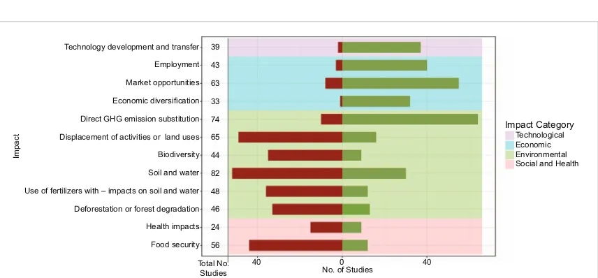
Technology development and transfer

Employment

Market opportunities

Economic diversification

Direct GHG emission substitution

Displacement of activities or land uses

Biodiversity

Soil and water

Use of fertilizers with – impacts on soil and water

Deforestation or forest degradation

Health impacts

Food security

Total No. Studies

Impact

40 56 24 46 48 82 44 65 74 33 63 43 39

0 40

Technological Economic Environmental Social and Health

Impact Category

No. of Studies

Figure 7.Distribution studies discussing negative and positive impacts for key side-effects. Adapted from Robledo-Abadet al(2017).

potentials (Krey et al 2014a, Smith et al 2016a,

Creutziget al 2015). 1 EJ of biomass typically yields around 0.02–0.05 GtCO₂worth of negative emissions. Total bioenergy potential estimates for 2050 range from 60–1548 EJ yr−1. Estimates at the lower-end of this range (Kraxner and Nordstr¨om2015, Searle and Malins2015, Smithet al2012) all provide minimum estimates of around 60 EJ yr−1. Bioenergy crop deploy-ment is limited by land allocation for natural parks (Kraxner and Nordstr¨om2015, Fieldet al2008(a 2030 estimate)), or when deployed only on degraded (Wicke

et al2011, Nijsenet al2012) or marginal land (Searle and Malins2015), which will lead to lower yields. Other conservative estimates for 2050 consider only residues, either immediately available (Smithet al2012) or in line with 2050 estimates (Tokimatsuet al2017).

Potentials increase as deployment constraints are relaxed to include more productive land, with

mini-mum potentials of 130 and 160 EJ yr−1and maximum

estimates of 216 and 267 EJ yr−1(Beringeret al2011,

Rogner et al 2012) and similar estimates for 2055

are characterized by more limited cropland expansion and lower nature conservation criteria.

The group of optimistic estimates start at around

350 EJ yr−1 (Cornelissen et al 2012, Fischer and

Schrattenholzer 2001, Smeets et al 2007). Although Cornelissen’s calculations are limited to rain-fed agri-culture, and apply a food-first principle, they still estimate 340 EJ available/yr by 2050. This is partly due to their inclusion of algae as a feedstock, which contributes 90 EJ yr−1 to their estimate and the use of fertilizers over a relatively large deployment area (673 Mha). Fischer and Schrattenholzer (2001) assume limited agricultural land expansion due to increasing yields. Bioenergy crops here are deployed on grassland rather than constrained to marginal or degraded lands as in the more conservative estimates above. Smeets

et al (2007) provide the most optimistic estimates

between 370–1500 EJ yr−1. Much of this potential

(215–1272 EJ yr−1) comes from dedicated bioenergy

crops and the wide range reported reflects different factor yield increases (2.9 vs 4.6), area available for deployment (729 Mha and 3585 Mha respectively) and rainfed vs irrigated agriculture. Smith (2012) provides an estimate of biospheric capacity of 727.5 EJ yr−1over all vegetated land (11 000 Mha). Rogner et al (2012) assess a theoretical bioenergy potential of 793 EJ yr−1 if all aboveground net primary production (NPP) that is not used for food, feed or fiber is devoted to bioenergy production.

Bioenergy estimates from dedicated crops offer wide discrepancies, from conservative estimates of approximately 20 EJ yr−1(Erbet al2012a, Thr¨anet al 2010, Hakala et al2008, Nijsen et al2012, Beringer

et al 2011), to middle ranges of 70–180 (Erb et al

2012b, Yamamoto et al 2000, Hoogwijk et al 2009,

Cornelissenet al2012, Beringer et al2011, Thr¨anet al2010, Rogner et al2012) to high estimates above 200 EJ yr−1 (Hoogwijket al 2005, Smeetset al 2007, Cornelissenet al2012). Variance depends largely on available land and yields (Dornburget al2010, Boysen

et al2017), which in turn can be driven by assump-tions regarding future population and diet (Haberl

et al2011, Hakala et al2008), biodiversity and con-servation restrictions (Erbet al2012a, Beringer et al 2011, Poppet al2011), or land quality and technology improvements (Smeetset al2007). Hakala’s low esti-mates use current global statistics rather than projected yields to account for social and institutional condi-tions, and they further reduce their estimates when considering global affluent diets (Hakalaet al 2008). High estimates are derived from scenarios of large-scale deployment on abandoned agricultural land, where yield factor increases are far higher than on

marginal lands (Smeets et al 2007, Hoogwijk et al

2009). Higher estimates are commonly grounded in

economic analysis, involving factors such as tech-nological change to improve yields, whereas lower estimates focus on ecological and biophysical concerns

and natural limits to sustainable bioenergy deployment (Creutzig2016).

Estimates for forestry-sourced bioenergy range

from 38–165 EJ yr−1 (Smeets and Faaij 2007, Lauri

et al2014, Smeetset al2007, Cornelissenet al2012, Rogneret al2012). The only estimate above 200 EJ yr−1 comes from an aggressive deployment of afforestation and reforestation activities. Smeets’ central estimate sees forests being deployed on 292 Mha of land, while Obersteineret al(2006)’s lower deployment scenario starts at 290 Mha and goes up to 660 Mha for the extreme estimate of 1250 EJ yr−1. By contrast, the lowest estimate comes from the application of strict sustainability criteria that excludes consideration of protected, inaccessible and undisturbed forests, as well as non-commercial species and traditional-use biomass resources (Cornelissenet al2012).

Although not fully assessed here, algae has been proposed as an alternative source of biomass for BECCS. Due to its high photosynthetic efficiency and

high yields (Moreira and Pires 2016), its capacity

to co-produce protein and its potential to decrease

land competition (Beal et al 2018), algae may

address some of the sustainability concerns raised by BECCS.

Global storage potentials.The second major factor that could restrict BECCS deployment is the availabil-ity of storage. There is little doubt in the literature that there is, in principle, sufficient potential avail-able across the globe to geologically store vast amounts of CO₂permanently, as required by many 1.5◦C and 2◦C scenarios (Dooley2013). Yet in individual regions there could be storage bottlenecks that would limit the BECCS potential in that region (Calvinet al2009, Edmondset al2007, Dooley2013).

Global estimates of total storage potential span

a massive range—from 320 (Koide et al 1993) to

50 000 GtCO₂(Hendriks and Blok1995). Global esti-mates using top down approaches grow as more storage options are considered. The low estimate of 320 GtCO₂conservatively assumes that 1% of all sed-imentary basins might be suitable for storage (Koide

et al1993). This more than doubles (to 777 GtCO₂) when proven depleted oil and gas reserves are included (Ormerodet al1993), then roughly doubles again to 2065 GtCO₂(Hendriks and Blok1995) when consider-ing undiscovered oil and gas reserves. The assessment

increases dramatically to over 50 000 GtCO₂ when

other trapping mechanisms allow storage to occur in aquifers without a structural trap (Hendriks and Blok1995). Later estimates make use of more detailed information from regional and national studies to generate global estimates (Selosse and Ricci2017, Doo-ley 2013). Dooley’s estimate of theoretical capacity

is in the same order of magnitude (35 000 GtCO₂),

but is significantly reduced by physical and

practi-cal constraints to 13 500, 3900 and 290 GtCO₂ of

respectively22_{. The effective capacity estimate is in line}

with estimates reached by integrating global IEA GHG data with data from national and site specific esti-mates, and other sources such as Total Petroleum System and the United States Geological Survey for a total potential of 10 000 GtCO₂(Selosse and Ricci

2017).

Global estimates for depleted oil and gas fields range

from 458 (Ormerod et al1993) to 923 GtCO₂(IEA

Greenhouse Gas R&D Programme2000) (IEA

Green-house Gas R&D Programme 2000). This relatively narrow range likely results from thorough documen-tation of structures during exploration and extraction. Despite wide differences in total potentials, the broad studies with breakdowns provide a narrower range of 458–801 for oil and gas fields (Hendriks and Blok

1995, Selosse and Ricci 2017, Ormerod et al 1993). IEA GHG estimates are based on a detailed database of 155 geological provinces (IEA Greenhouse Gas R&D Programme2000). Regional assessments provide insight into the geographical distribution of resources. North American estimates range from 40 (Dooley

et al2005) to 136 GtCO₂(Wrightet al2013). The low estimate only considers the CO₂sequestration poten-tial of depleted gas fields and oil fields with enhanced oil recovery (EOR). European estimates range from the effective capacity evaluated by the GeoCapacity project of 20 GtCO₂(Vangkilde-Pedersenet al2008)

to 280 GtCO₂ (Hendriks and Blok1995). The latter

estimate can likely be attributed to the former Soviet Union nations, which Selosse and Ricci (2017) estimate

have 277 GtCO₂ of capacity. Estimates that exclude

this region cluster are between 20 and 60 GtCO₂

(Vangkilde-Pedersenet al2008,2009, IEA GHG2005, Selosse and Ricci2017). Lower estimates exclude some countries and present effective capacities with site-specific information. Middle Eastern estimates range from 208 (Selosse and Ricci2017) to 250 GtCO₂

(Hen-driks and Blok 1995), but only EOR estimates were

found at national or site specific levels (Jajuet al2016, Movagharnejadet al2012, Mortensenet al2016, Has-saniet al2016).

Estimates of the storage potential of coal beds range from 60 (Gale and Freund2001, Gale2004) to 700 GtCO₂(Kuuskraaet al1992). Lower estimates con-sider the economic constraints (Dooleyet al2005) of 10 high potential countries, while a more comprehen-sive assessment of 24 countries expands the potential

to 487 GtCO₂ (Godec et al 2014). Kuuskraa et al

(1992)’s estimate appears to be based on theoretical analysis by the authors leading to a higher range. The early estimate of 150 GtCO₂ considers few countries and subsequent regional estimates have revised this

22 _{The types of potential correspond to estimates of capacity}

increas-ingly constrained by physical (theoretical), technical (effective), regulatory, economic (practical) barriers as well as detailed matching with large CO₂sources (matched) (Bradshawet al2007, Bachuet al 2007).

upward. In North America, estimates have increased

from 47 GtCO₂ (IEA GHG 1998, Gale 2004) to

65–120 GtCO₂(Godecet al2014, Dooleyet al2005, Wrightet al2013). Lower-end estimates tend to con-sider specific basins with high potential and favorable market conditions while higher estimates reflect theo-retical global potentials.

Most of the potential and variability in esti-mates comes from estiesti-mates of potentials in aquifers. Hendrik’s broad estimate of 200–50 000 GtCO₂ cov-ers all other estimates in the literature. The lower-end considers aquifers only with a structural trap, while the high end integrates other trapping mechanisms

allowing much wider deployment23_{. Early estimates}

are explicitly conservative, but it is unclear whether they are considering structural traps in their constraints (Koide et al 1993). Although the 50 000 estimate is explicitly theoretical, regional estimates have provided support to it. High potentials have been estimated

for North America (Dooleyet al 2005, Wright et al

2013), China (Li et al 2009) and OECD Europe

(IEA GHG2005).

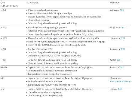
Costs.Cost estimates through the entire literature

range from US$15–400/tCO₂. Estimates that cover

BECCS generally estimate prices of between US$30

and 400/tCO₂ (Luckow et al 2010, Koornneef et al

2012, Arastoet al2014). However, most sources focus

on a specific source for CO₂ capture. Many papers

explore the potential of capture from ethanol fermen-tation and find ranges of US$20 to 175/tCO₂(de Visser

et al2011, Fabbriet al2011, Fornellet al2013, Laude

et al2011, M¨ollerstenet al2004, Johnsonet al2014,

Rochedo et al 2016). Low values within the studies

represent deployment in the most suitable plants with easy access to abundant biomass and short distances to storage sites. Capturing CO₂emissions from both ethanol fermentation and cogeneration units increases

costs (US$40–120 vs US$180–200/tCO₂ avoided)

but also increases avoidance potential (Laude et al

2011). Combustion BECCS has higher costs ranging

from US$88 to US$288/tCO₂(Akgulet al 2014, Al-Qayimet al 2015, K¨arki et al 2013). Low estimates in combustion come from utilizing oxy-fuel technolo-gies (Al-Qayim et al 2015, K¨arki et al 2013). The lowest estimate for this technology group (US$14– 77/tCO₂avoided) comes from a variation of oxy-fuel

combustion that is still unproven (Abanades et al

2011). Biomass gasification technologies are estimated

between US$30 to US$6/tCO₂ (Gough and Upham

2011, Rhodes and Keith 2005, Sanchez and

Call-away 2016). However, Ranjan provides much more

pessimistic estimates of US$150–400/tCO₂ avoided,

but these might be due to extremely large land requirements for the production of biomass. The cost

23_{Structural traps refer to geological structures capable of}

of CO₂avoidance via BECCS utilizing black liquor pro-duced by pulp and paper mills has been estimated to

range between US$20 and US$70/tCO₂ when using

recovery boilers (Onarheim et al 2015, M¨ollersten

et al 2004) and US$20–55 when using gasification

technologies (M¨ollersten et al 2006, 2004). Other technologies have been estimated at US$86–167/tCO₂ avoided (Carboet al2011) and US$20–40/tCO₂ (John-sonet al 2014) for BioSNG and biomass FT diesel, respectively.

Low cost estimates typically start with a coal-CCS configuration and assume biomass fuel costs lower than those of coal, as at least partially available, e.g. in the US-Midwest. Transport costs of biomass are included in some (e.g. Sanchez and Callaway2016) but not all studies. Importantly, biomass is nearly always assumed to be produced at zero cycle emissions. But life-cycle emissions related to direct or indirect land use pose a 10%–30% efficiency penalty on carbon abate-ment, and hence on costs of negative emissions, even in the optimistic cases where biomass is derived from cel-lulosic sources or dedicated bioenergy crops. It may also be relevant to price in indirect externalities, mediated via land markets, e.g. on food markets, ecosystem ser-vices, and livelihoods (see below). This is a contentious exercise with little agreement and large parameter uncertainties.

Side effects. Side effects can be broadly cat-egorized into climate effects induced by biomass provision, resource needs, and broader environmental and sustainability effects transmitted via the coupled

land-energy system (Creutzig et al 2015,

Robledo-Abad et al2017). An exhaustive and comprehensive literature review of 1175 publications on side effects and sustainable development contributions of bioen-ergy published in a recent study revealed that side effects can be in general both positive and negative; however, negative effects are more often observed in the literature in social and environmental dimen-sions, whereas positive effects are more often observed in economic and technological dimensions (Robledo-Abadet al2017).

Climate effects belong to the categories of direct land use change, indirect land use change, and albedo effects. Land use change emissions include those from change in previous use, such as deforestation, and changes in global land use induced by economic markets. These are generally high for first-generation biofuels, such as corn ethanol, which are derived from food markets; while overall emissions are still rele-vant but in lower ranges for bioenergy from cellulosic or woody sources, and from food waste and forest residues (Plevinet al2010, Smithet al2016a)24_{. (Some}

24_{Although achievable scales are not clear yet, there is also research}

on third-generation biofuels, derived from algal biomass (Brennan and Owende2010) with the potential to enhance yields by improv-ing microalgal biology through genetic or metabolic engineerimprov-ing (Tandon and Jin2017).

specific albeit relatively low-yield choices can gener-ate carbon-negative bioenergy, see Tilmanet al2006). Low emissions also translate into a significant effi-ciency loss in bioenergy for climate mitigation or for BECCS as negative emissions technologies. Calcula-tion of indirect land use effects is subject to parameter and structural model choice rather than accounting only and leads to considerable uncertainty in estimates and abatement effects (Plevinet al2010,2014).

The global albedo effects of cultivating biomass for bioenergy are also relevant and vary with geograph-ical location. Higher latitudes, where biomass might replace reflective snow cover, are more prone to an albedo effect that offsets climate mitigation (Brightet al 2015). Land use and land cover change forcing ranges

from −0.06 to−0.29 W m−2 by 2070 depending on

assumptions regarding future crop yield growth and whether climate policy favors afforestation or bioenergy crops (Joneset al2015).

Required resources may include fertilizer use (which in turn lead to GHG emissions and must be fac-tored in) and water use. If 170 EJ yr−1were produced

by a 2◦C-compliant BECCS infrastructure by 2100,

the water footprint would amount to 59.5 km3/GtCO₂

by 2100 (Smith2016), which corresponds to 1.5% of

global yearly freshwater withdrawals.

Bioenergy is confronted with substantial con-cerns regarding competition for land, including impact on food prices, biodiversity, water and nutrients

(Williamson 2016, Smith et al 2013, Haberl 2015,

Robledo-Abad et al 2017, Edenhofer et al 2013). A

major concern is the effect that large-scale deployment poses on food security. Although many studies apply a food-first principle to limit deployment, increased land competition could lead to increased global food prices (Poppet al2011, Reillyet al2012) and regional resource shortages (M¨ulleret al 2008). Some biofu-els (such as corn ethanol) impact food prices, but others that do not directly compete with food (such as sugarcane) have a lower impact—yet often these price impacts are dwarfed by exogenous factors like

economic growth (Zilbermanet al2013, Roberts and

Schlenker 2010, Timilsina et al 2012). These

con-cerns can be alleviated by limiting deployment to marginal land, but this is often associated with detri-mental impacts on biodiversity (Daleet al2010, Wiens

et al 2011). Conversely, deployment on degraded lands could contribute to protection from erosion and soil restoration (Lemus and Lal2005).

More than 1 billion small-holder farmers could also be directly or indirectly subjected to changing agricultural practices and bioenergy systems, both pos-itively and negatively (Mutopo et al 2011, Creutzig

a local energy supplement and the consolidation of cor-porate power in agribusiness and energy sectors (Borras and Franco2010, Rist et al2010). Case study analy-ses demonstrate that while some local actors are likely to profit from bioenergy deployment schemes, oth-ers, often starting from an institutionally disadvantaged position, can lose out (Creutziget al2013, Schoneveld

et al2010). Distributional issues are hence a crucial dimension in designing the governance of bioenergy (Hunsbergeret al2014).

CCS poses its own set of risks. Overpressure could lead to the pollution of potable water, to seismic activity or to leaks, which could not only rapidly reverse pos-itive mitigation effects, but cause environmental and

health damage at the leakage sites (Holloway 2009,

National Academy of Sciences2015, Smithet al2016a, Bruckneret al2014).

Permanence and saturation. In principle, once the

CO₂removed from the atmosphere via BECCS is

geo-logically stored, it is one of the NET options that is less vulnerable to reversal. Most importantly, stored CO₂is not subject to further management decisions like other land-based NETs. While leakage can be an issue, it is not widely perceived as a major hurdle to safe and perma-nent storage. Moreover, there is significant research on monitoring and verification as well as on leak detection and remediation (Buiet al2018). However, consider-able concerns with BECCS are associated with its level of effectiveness, which can be compromised by sig-nificant amounts of emissions from indirect land-use change (Plevinet al2010).

Authors’ assessment. Overall, by 2050 we see BECCS at costs of US$100–200/tCO₂that accrue inter alia from the necessity to guarantee limited sustainabil-ity and land-use carbon cycle effects, and which will require high management intensity on a case-by-case basis. Our estimate of 2050 potentials ranges is 0.5– 5 GtCO₂ (considering here a technological potential that remains cognizant of other sustainability aims). As for all land-intensive options, we remain conservative in our suggested values as they refer to mid-century where population pressures are highest according to recent projections (Samir and Lutz2017). A range of 5GtCO₂and possibly higher requires global land gov-ernance, integrating multiple land use concerns for the global common good.

3.2. Afforestation and reforestation (AR)

Afforestation refers to planting trees on land that has not been afforested in recent history (a reference value of at least 50 years is commonly used). Reforestation, on the other hand, refers to the replanting of trees

on more recently deforested land (IPCC2000).

Neg-ative emissions can arise from both practices, as the growth of additional biomass sequesters CO₂from the atmosphere. The distinction between afforestation and reforestation is often not clean in the literature and we therefore categorize them jointly.

Global sequestration potentials and costs.Out of 12 previous assessments of different NETs, seven offer yearly potentials at either mid-century or 2100. The 2050 range is 0.5–7 GtCO₂yr−1(Lenton2014), which encompasses the ranges given in earlier assessments

(Friends of the Earth 2011, McLaren 2012, Lenton

2010). In 2100, this range widens to 1–12 GtCO₂yr−1,

covering the ranges given by Smith et al (2016a),

the National Academy of Sciences (2015) and Lenton (2010,2014). In addition, some assessments give poten-tials in cumulative terms with the lowest 2100 estimate

of 80 GtCO₂ coming from the Oxford University’s

Stranded Assets Programme (Caldecottet al2015) and the highest estimate being the upper end of the IPCC

AR5 range with 260 GtCO₂ (IPCC 2014a). There is

high agreement on the maximal costs of AR being around US$100/ton of sequestered CO₂and less agree-ment on the lower-end of the range, with the National Academy of Sciences (2015) quoting US$1 and the rest

being in a range of US$18–20/ton CO₂. The Royal

Society Report (2009) does acknowledge AR as an

option to remove carbon, but does not give potentials. Their assessment points to‘low costs’as well.

Taking the systematically scoped literature (see section 3.2.1) into account, the upper end of the 2100 sequestration potential remains at just above 12 GtCO₂yr−1in 2100. The lower-end is slightly more conservative at 0.54 GtCO₂yr−1(Liuet al2016)25_{. New}

estimates from Integrated Assessment Modeling com-bined with more detailed bottom-up land use models

give a range of 5.83–9.56 GtCO₂yr−1 in 2100 when

2580 Mha are afforested (Kreidenweiset al2016), with a lower potential of 3.53 GtCO₂yr−1 for

afforesta-tion of 1489 Mha at a carbon price of US$24/tCO₂

(Humpen¨oder et al 2014). Earth System Modeling

mimicking the afforestation rates in an RCP4.5 path-way finds 6.64 GtCO₂yr−1in 2100 (Sonntaget al2016).

Houghton et al(2015) estimate that about 500 Mha

could be available for the re-establishment of the world’s tropical forests on lands previously forested but not currently used productively. This would sequester at least 3.7 GtCO₂annually for decades, even though they raise the important caveat that forests need both time to grow and will eventually suffer from saturation and thus assume a linear decline in productivity from 3.7 GtCO₂in 2065 to 0 by 2095. Earlier estimates lie in between 0.47 and 4.88 GtCO₂yr−1by 2100

(Sohn-gen and Mendelsohn 2003, Cannell 2002, Canadell

and Raupach 2008, Strengers et al 2008, van

Min-nenet al 2008, Thomson et al2008) with estimates depending on various assumptions, most notably the amount of land available. For example, many stud-ies assume that only abandoned or low-productivity

land can be used for AR. For example, Thomsonet al

(2008) use an area of 120 Mha of unproductive land