Using Polytrees
.
White Rose Research Online URL for this paper:
http://eprints.whiterose.ac.uk/115224/
Version: Accepted Version
Proceedings Paper:
Fehri, H., Gooya, A., Johnston, S.A. et al. (1 more author) (2017) Multi-class Image
Segmentation in Fluorescence Microscopy Using Polytrees. In: Information Processing in
Medical Imaging. International Conference on Information Processing in Medical Imaging,
25/06/2017 - 30/06/2017, Appalachian State University, Boone, North Carolina. Springer,
Cham , pp. 517-528. ISBN 978-3-319-59049-3
https://doi.org/10.1007/978-3-319-59050-9_41
[email protected] https://eprints.whiterose.ac.uk/
Reuse
Unless indicated otherwise, fulltext items are protected by copyright with all rights reserved. The copyright exception in section 29 of the Copyright, Designs and Patents Act 1988 allows the making of a single copy solely for the purpose of non-commercial research or private study within the limits of fair dealing. The publisher or other rights-holder may allow further reproduction and re-use of this version - refer to the White Rose Research Online record for this item. Where records identify the publisher as the copyright holder, users can verify any specific terms of use on the publisher’s website.
Takedown
If you consider content in White Rose Research Online to be in breach of UK law, please notify us by
Microscopy Images Using Polytrees
Hamid Fehri1,2,3, Ali Gooya1, Simon A. Johnston2,3, and Alejandro F. Frangi1( )
1 Center for Computational Imaging Simulation Technologies in Biomedicine
(CISTIB), The University of Sheffield, Sheffield, United Kingdom
2 Bateson Centre, Firth Court, University of Sheffield
3 Department of Infection, Immunity and Cardiovascular Disease, Medical School,
University of Sheffield
Abstract. Multi-class segmentation is a crucial step in cell image analy-sis. This process becomes challenging when little information is available for recognising cells from the background, due to their poor discrimina-tive features. To alleviate this, directed acyclic graphs such as trees have been proposed to model top-down statistical dependencies as a prior for improved image segmentation. However, using trees, modelling the rela-tions between labels of multiple classes becomes difficult. To overcome this limitation, we propose a polytree graphical model that captures label proximity relations more naturally compared to tree based approaches. A novel recursive mechanism based on two-pass message passing is devel-oped to efficiently calculate closed form posteriors of graph nodes on the polytree. The algorithm is evaluated using simulated data, synthetic im-ages and real fluorescence microscopy imim-ages. Our method achieves Dice scores of 94.5% and 98% on macrophage and seed classes, respectively, outperforming GMM based classifiers.
1
Introduction
Macrophages are cells that play vital roles within the immune system. They recognise invasions to body and combat their agents and are also involved in healing processes. Studying these cells in depth requires quantification of their behaviour in their interactions with other cells and proteins, which needs seg-mentation of cells in microscopy images. One instance of such studies is the segmentation of nuclear and surface areas of mice macrophages in fluorescence microscopy images [9], which defines a multi-class segmentation problem ad-dressed here. The challenges are more highlighted when limited information is available for recognition of each area, due to the low quality of images and/or complexity of shapes. In these cases, quality of segmentation is subject to im-provement by employing inter-object relations.
while the other one estimates density based on regression [1]. Former approaches perform based on a prior segmentation or detection of individual cells, while the latter do not rely on individual object detection and rather take a holistic ap-proach towards counting and have been proven to be more efficient. Inspired by the counting application outlined in [1], our segmentation method is capable of extracting the image foreground as the union of subregions having different labels. The segmented foreground can be further used for efficient recognition of individual cells and their nuclei through post processing steps.
Graphical models are tools for modelling associative relations between ob-jects. The key aspect of these models is that the label of each node is determined based on both its own attributes as well as attributes of other nodes connected to it through graph edges. This way, not only all the relevant information is in-corporated in inferring the labels, but also label configuration constraints can be effectively projected on the model and be used during the inference. For instance, Chen et al. [5] employed graphical models to incorporate nuclear positions with boundary information for yeast cell segmentation. In a broader context of appli-cation, Uzunbas et al. [12] used an interactive graphical-model-based approach which seeks user’s input for nodes with uncertain labels and learns from mis-labelled nodes. Another instance is the use of graphical models for combining appearance models with shape priors for retinal segmentation [11].
Two types of graphical models have been used for image segmentation. Markov Random Fields have weighted edges indicating the degree of dependen-cies between variables. These models require iterative procedures for estimating the hidden random variables and are therefore computationally demanding [4] and only approximate solutions are achievable for them [7]. On the other hand, Bayesian Networks (BNs) have directed edges that show how random variables depend on each other. Laferte et al. [8] proposed an efficient posterior calcu-lation algorithm for nodes on a tree BN using message passing. Tree BNs are models in which there is only one route between any two nodes, and each node (except the root node) has exactly one parent node. Despite the efficiency of their proposed model, it lacks the ability to model complex multi-label configu-ration constraints. More specifically, the tree model proposed in [8] is capable of modelling two-wise constraints between nodes and thus suitable for binary im-age segmentation. However, many applications, such as cell/nuclei segmentation involve more complex constraints due to the presence of multiple classes.
evaluated by ancestral sampling on arbitrary graphs, and applied on synthetic and real microscopy images to segment macrophages and nuclei (seeds) from background. However, we anticipate that more general applications of polytrees using the proposed inference algorithm.
2
Method
Here, the procedure of using our proposed graphical model for image segmenta-tion is presented. First, a polytree is generated for the image by grouping similar pixels and regarding them as nodes of the graph. Next, the parameters of the likelihood functions are trained and labels of the nodes are inferred. Finally, the segmented image is constructed based on the optimal labels on the graph.
ℒ: Leaf node
ℛ: Root nodes (lowest level) Initial superpixels
(a)
! 2
3
3
1 2
�
� �
(b)
�∀ �∀#
�∀
∃
% �∀
& %
�∀∋
(c)
�∀ �∀#
�∀∃% �∀&% �∀∋
�∀ �∀∋
�∀∃%
�∀#
�∀&%
(d)
�∀
�∀
#
∃ �∀
% ∃
(e)
�∀
�∀
#
∃ �∀
% ∃
[image:4.612.149.468.299.510.2](f)
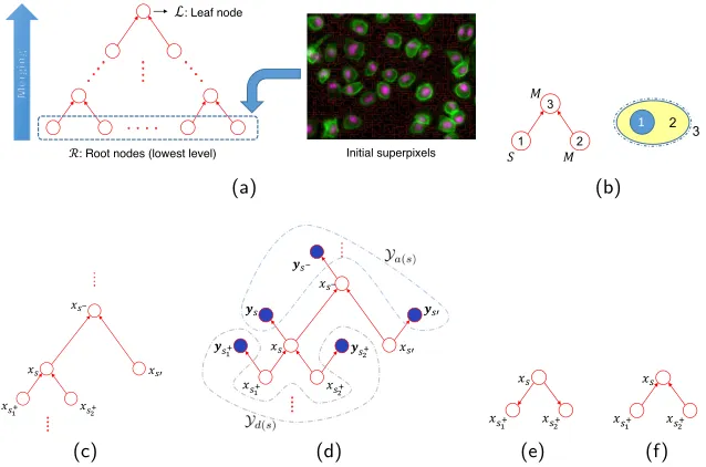
Fig. 1.Graph generation and inference on the polytree. (a) Generation of the polytree for the sample image. (b) Symbolic process of node merging for a synthetic macrophage with a seed. (c) Presenting the notation for nodes connected to an internal nodesof the graph. (d) Graphical representation of ascendant,Ya(s), and descendant,Yd(s),
obser-vation nodes. Edge directions on cliques in conventional directed tree graphical models and the proposed polytree structure are shown in figures (e) and (f), respectively.
2.1 Graph generation
algorithm [2], which refines the initial grid of identically block shaped superpixels into more coherent ones. The two most similar superpixels are then recursively merged to generate nodes in higher levels of the hierarchical graph, as follows.
Firstly, for each superpixel at the finest level, one (root) node in the lowest level of the graph is created (see Fig. 1a). Each two nodes that achieve the highest score in a similarity metric are then merged to create a new node. The new node corresponds to the union of image regions attached to its two lower level descendant nodes. We define the similarity metric as a superposition of distances using spatial and intensity features of the superpixels. A vector β is introduced to adjust contributions of each of these features in the similarity metric. The choice of β is investigated in section 3.3. After each merging step, the new node and all the other orphan nodes, are assessed with the similarity metric to recognise candidate nodes for the subsequent merging step. Region merging is continued until only two orphan nodes remain in the graph, which are eventually merged to create the leaf node that corresponds to the whole image (Fig. 1a). It is worth mentioning that since two nodes are merged at each step of graph evolution, the resulting structure is a binary graph; i.e. each non-root node has exactly two descendent nodes directly connected to it. We call this three-wise structure a clique and denote it byparent1−child−parent2.
Once the graph is generated for the image, a set of observed and latent vari-ables are assigned to nodes to define of the inference problem, which is presented in the next section. Fig. 1b shows a symbolic process of merging for a cell with a seed. Nodes 1 and 2 align with blue and yellow areas in the synthetic cell. If these two nodes are chosen to be merged based on their value in the similarity metric, node 3 is generated which corresponds to the union of blue and yellow areas and is annotated by the dashed ellipse. This clique is represented by 1−3−2.
2.2 Label inference
Let X = {xs} and Y = {ys} denote sets of labels (latent variables) and the corresponding observed features at nodes, respectively, andG denote the set of nodes and edges. We assume that each node can be labelled as background (B), macrophage (M) or seed (S). Equivalently, xs ∈ Λ, where Λ is the set of all possible labels, Λ = {B, M, S}. Following the notation of [8], for an internal node (neither in the lowest level nor the leaf node) sin the graph, s−
,s+ and s′ denote nodes in higher, lower and same layers, respectively (Fig. 1c).
Fig. 1e shows the structure of a clique in conventional trees [8], where graph edges are oriented accordingly from the root node s to the leaves s+1, s+2. For this configuration, the joint probability factorises into probabilities of 1-1 child-parent constraints, as p(X) = p(xs+
1|xs)p(xs +
2|xs)p(xs). The limitation of this
having oneM and oneSparent nodes, as depicted in Fig. 1b. In the conventional structures, this prior knowledge is projected on the model through setting the probabilitiesp(xs+
i =S|xs =M) and p(xs
+
i =M|xs=M) to non-zero values.
However, enforcing the former constraint also makesS−M−S cliques feasible, even though they are not acceptable based on the nature of the problem. This example shows the shortcoming of conventional directed tree models.
To overcome this limitation, we propose the use of another type of hierarchi-cal graphihierarchi-cal models with reverse edge orientations, as depicted in Fig. 1f, hierarchi-called
polytrees [3]. In a polytree, each node at the lowest graph level (finest image
res-olution) is a root (in contrast to the single root node in conventional tree graphs) and there is only one leaf node (see Fig. 1a). This subtle yeteffective change re-places 1-1 child-parent constraints with three-wise constraints on the cliques. The joint probability in this case is factorised asp(X) =p(xs|xs+
1, xs
+
2)p(xs
+
1)p(xs
+
2),
in which the termp(xs|xs+
1, xs
+
2) enforces the constraint on the clique. Using this
configuration, the example structure of Fig. 1b requires setting the constraint p(xs =M|xs+
1 =S, xs
+
2 =M) to be nonzero. However, in contrast to the
pre-vious structure, enforcing this constraint does not give rise to the emergence of physically infeasible clique structures.
We now derive equations governing the posterior probabilities of graph nodes. Given the observed dataY, finding the best segmentation is equivalent to infer-ring the best configuration of labelsXfor the graph. Bayesian inference associates the most probable label from the set of possible labelsΛ, given all observations:
∀s∈ G,xsˆ = arg max xs∈Λ
p(xs|Y) (1)
As the dependencies of nodes’ labels have been revised in the proposed graph structure, a new set of equations are derived to calculate the closed-form poste-rior probabilities at each node. The inference algorithm on the polytree calcu-lates the posteriors in two passes. These two consist of a pass from the leaf to the roots, (top-down pass), and from the roots to the leaf (bottom-up pass).
Probability of a node’s labelxs, given all data Y, is computed by marginal-ising the probability of the clique over two parent nodess+1 ands+2 givenYand is called joint posterior.
p(xs|Y) = X xs+
1
,xs+ 2
p(xs, xs+
1, xs
+
2|Y) (2)
Here, three-wise constraints on cliques appear in the posterior calculation. Using the D-separation rule [10], the joint posterior is expanded as follows:
p(xs, xs+
1, xs
+
2|Y) =p(xs|xs
+
1, xs
+
2,Y)p(xs
+
1, xs
+
2|Y)
=p(xs|xs+
1, xs
+
2,Ya(s))p(xs
+
1, xs
+
2|Ya(s
+
1,s
+
2),Yd(s
+
1,s
+
2))
(3)
nodes refer to the set of all nodes that are connected to s (S) through edges with inward directions. Similarly, descendant nodes include the nodes that are connected to nodes(S) through outward oriented graph edges. The union of as-cendant and desas-cendant observation nodes constructs the set of all observations (see Fig. 1d for a graphical explanation).
We first elaborate the term p(xs|xs+
1, xs
+
2,Ya(s)) on the right-hand side of
Eq. 3. This term enforces posteriors of infeasible configurations to zero, as it is a product of the joint probability of a child node and its two parent nodes.
p(xs|xs+
1, xs
+
2,Ya(s)) =
p(xs, xs+
1, xs
+
2|Ya(s))
P
x′sp(x
′
s, xs+1, xs +
2|Ya(s))
(4)
Using D-separation rule, the nominator becomes:
p(xs, xs+
1, xs
+
2|Ya(s)) =p(xs
+
1, xs
+
2|xs)p(xs|Ya(s))
= p(xs, xs
+
1, xs
+
2)
p(xs) p(xs|Ya(s)).
(5)
Term p(xs, xs+
1, xs
+
2) in Eq. 5 controls the occurrence of feasible and infeasible
configurations on the graph, by being set to zero and nonzero values for them, respectively. Term p(xs|Ya(s)) in Eq. 5 is the posterior of node s having given observations of all its ascendant nodes as well as its own observation. This
top-down posterior is expanded as:
p(xs|Ya(s))∝
X
xs−,xs′
p(ys|xs)p(ys′|xs′)p(xs′|Yd(s′))
p(xs, xs′, xs−) p(xs−)p(xs′)
p(xs−|Ya(s−))
(6) Eq. 6 indicates that having calculated the likelihood probabilities p(ys|xs) andp(ys′|xs′) and the posteriorp(xs′|Yd(s′)), the top-down posterior of nodesis calculated based on top-down posterior of nodes−. This implies that a top-down recursion calculates the top-down posteriors for all nodes.
On the other hand, term p(xs+
1, xs
+
2|Ya(s
+
1,s
+
2),Yd(s
+
1,s
+
2)) on the right-hand
side of Eq. 3 is factorised by several usages of D-separation rule. This factorisa-tion separates parts that are calculated from ascendant and descendant nodes.
p(xs+
1, xs
+
2|Ya(s
+
1,s
+
2),Yd(s
+
1,s
+
2))∝p(Ya(s
+
1,s
+
2),Yd(s
+
1,s
+
2)|xs
+
1, xs
+
2)p(xs
+
1, xs
+
2)
=p(Ya(s+
1,s
+
2)|xs
+
1, xs
+
2)p(Yd(s
+
1,s
+
2)|xs
+
1, xs
+
2)p(xs
+
1, xs
+
2)
=p(Ya(s+
1,s
+
2)|xs
+
1, xs
+
2)p(Yd(s
+
1)|xs
+
1)p(Yd(s
+
2)|xs
+
2)p(xs
+
1, xs
+
2)
∝p(xs+
1, xs
+
2|Ya(s
+
1,s
+
2))
p(xs+
1|Yd(s
+
1))
p(xs+
1)
p(xs+
2|Yd(s
+
2))
p(xs+
2)
(7) Similar to Eq. 6, termp(xs+
1, xs
+
2|Ya(s
+
1,s
+
2)) on the right-hand side of Eq. 7
is calculated through a top-down recursion as below.
p(xs+
1, xs
+
2|Ya(s
+
1,s
+
2))∝
X
xs
p(ys+
1|xs
+
1)p(ys
+
2|xs
+
2)p(xs
+
1, xs
+
Using a definition similar to that of top-down posterior, termsp(xs+
1|Yd(s
+
1))
andp(xs+
2|Yd(s
+
2)) in Eq. 7 are calledbottom-upposteriors as they are calculated
based on posteriors of their descendant nodes. For each nodesin the graph, the bottom-up posterior is written as
p(xs|Yd(s))∝
X x s+ 1 ,x s+ 2
p(ys+
1|xs
+
1)p(ys
+
2|xs
+
2)
p(xs+
1|Yd(s
+
1))p(xs
+
2|Yd(s
+
2))p(xs|xs +
1, xs
+
2)
(9)
Derivations of Eq. 6, 8 and 9 are not included due to the shortage of space. Making use of Eq. 3, 4, 5 and 7 the node’s posterior in Eq. 2 given all the observations is written as follows.
p(xs|Y)∝ X
x s+ 1 ,x s+ 2
p(xs, xs+
1, xs
+
2|Ya(s))
P
x′sp(x ′
s, xs+1, xs +
2|Ya(s))
p(xs+
1, xs
+
2|Ya(s
+
1,s
+
2))
p(xs+
1|Yd(s
+
1))
p(xs+
1)
p(xs+
2|Yd(s
+
2))
p(xs+
2)
(10)
Eq. 10 calculates the posterior at each nodesusing three marginal posteri-orsp(xs, xs+
1, xs
+
2|Ya(s)),p(xs
+
1, xs
+
2|Ya(s
+
1,s
+
2)) andp(xs|Yd(s)), in Eq. 5, 8 and 9.
Each of these terms are calculated through either top-down or bottom-up recur-sions. The inference is summarised in Algorithm 1. Note that Rand L denote the set of root nodes and the leaf node in the graph, respectively.
3
Results
3.1 Validation of the inference algorithm in a two-class labelling
problem
To assess the performance of the core inference algorithm, regardless of the problem it is applied to, ancestral sampling was used [3]. This technique, which is applied to generative models, mimics the creation of the observed data by generating sets offantasydata. In this case, the model is a perfect representation of the observed data. Using the generated fantasy data as the observed data and comparing the inferred labels with the sampled values gives a measure for the method performance.
Consider we aim to draw a sample ˆx1,xˆ2, ...,xNˆ from the joint distribution p(X,Y). The graph consists of N nodes and xN denotes the only leaf node in the graph. To draw this sample, we start from the root nodes by taking samples ˆ
xs from the probability distribution p(xs)
s∈R for all root nodes. Visiting the internal nodes in an upward recursion, we draw a sample ˆxsfrom the conditional distribution p(xs|xs+
1, xs
+
2), for which the parent labelsxs +
1 and xs
+
2 have been
Algorithm 1Label inference on polytree directed graphical model
Preliminary pass. This initial upward recursion computes prior marginals for each node. p(xs|xs+
1
, xs+ 2
) are parameters set based on the nature of problem the model is representing.
for alls∈Rdo
p(xs) = |Λ1|
end for
for alls6∈Rdo
p(xs) =Px
s+
1
,x
s+
1
p(xs|xs+ 1
, xs+
2)
p(xs+
1)
p(xs+
2)
p(xs+ 1
, xs+
2|
xs) = p(xs|x
s+
1
,x
s+
2
)p(x
s+
1
)p(x
s+
2
)
p(xs)
end for
△ Bottom-up pass. Upward recursion for calculating bottom-up posteriors of nodes.
for alls∈Rdo
p(xs|Yd(s)) =p(xs)
end for
for alls6∈Rdo
p(xs|Yd(s))∝Px
s+
1
,x
s+
2
p(ys+
1|xs
+
1)p(ys
+
2|xs
+
2)p(xs
+
1|Yd(s
+
1))p(xs
+
2|Yd(s
+
2))p(xs|xs
+
1, xs
+
2)
end for
∇Top-down pass. Downward recursion for calculating top-down posteriors and calculation of complete posteriors from marginal posteriors.
if s=Lthen
p(xs|Ya(s)) =p(xs|ys)∝p(ys|xs)p(xs)
end if
for alls6=Ldo
p(xs|Ya(s))∝ P
xs−,xs′p(ys|xs)p(ys′|xs′)p(xs′|Yd(s′))
p(xs,xs′|xs−)
p(xs′) p(xs−|Ya(s−))
p(xs, xs+ 1
, xs+
2|Ya(s)) =
p(xs+ 1
, xs+
2|
xs)p(xs|Ya(s))
p(xs+ 1
, xs+
2|Ya(s
+
1,s
+
2))∝
P
xsp(ys+1|xs1+)p(ys+2|xs+2)p(xs+1, xs+2|xs)p(xs|Ya(s))
end for
0.2 0.4 0.6 0.8 1
x 0 2 4 6 8 10 (x|a,b)
a = 0.2 a = 0.4 a = 0.6 a = 0.8 a = 1
(a)
0.2 0.4 0.6 0.8 1
x 0 2 4 6 8 10 (x|b,a)
a = 0.2 a = 0.4 a = 0.6 a = 0.8 a = 1
(b)
101 102 103 104 105 Number of root nodes R 0
5 10 15 20
Percentage of error
a = 0.2 a = 0.4 a = 0.6 a = 0.8 a = 1
[image:9.612.135.472.511.605.2](c)
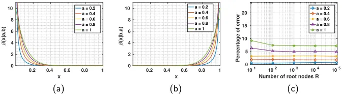
In this section only, we considered two classes for latent variables xs and selectingysfrom the continuous range [0,1] and beta distributions were used as class conditional likelihood functions, p(ys|xs). Labels done for different num-bers of root nodes ranging from 10 to 100000 (leading to 19 to 199999 nodes in total as the graph is binary) and for different selectivities of the likelihood functions, controlled by parameters ofβdistributions. Fig. 2a and 2b show beta distributions for different values of parameter a. Fig. 2c depicts percentage of nodes with wrongly inferred labels for different numbers of nodes in the graph and for different beta distributions. This experiment verifies the correctness of the developed derivations and also indicates that more selective likelihood dis-tribution functions result in higher inference accuracies. The best accuracy was achieved fora= 0.2 with the average error of 0.30%.
3.2 Validation of the algorithm on a synthetic image
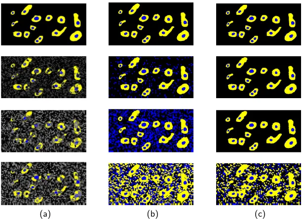
The method was evaluated on a synthetic image containing two types of objects. A multi-scale first and second order derivative based invariant features have been utilized here. The segmentation results were compared to those of using Gaussian Mixture Models (GMMs). Yellow and blue areas in the synthetic image represent macrophages and seeds, respectively (chosen to be similar to the real image dataset). At each node, median of intensity across the superpixel was utilised as feature. Random noise was added to these features. Random noise was added to feature values of each node, which were median of node’s intensity. Segmentation was done for different noise levels added to the synthetic image. Fig. 3 shows the synthetic image and its segmentation results for four cases of 0%, 30%, 60% and 65% of noise amplitudes, in each row, respectively. First column depicts the input image and second and third columns show results of segmentation for GMM and the proposed method, respectively. Dice scores of segmentations for GMM and the proposed method are shown in Fig. 4a. It can be seen that the proposed algorithm is more robust to intensive additive noise compared to GMM.
3.3 Applying the method to multi-class cell segmentation
(a) (b) (c)
Fig. 3. Segmentation of the synthetic image for different random noise levels using GMM and the proposed method. Rows of column (a) correspond to images, with 0%, 30%, 60% and 65% (of maximum image intensity levels), respectively. (b) and (c) show results of segmentation using GMM and the proposed method for the input images of the first column, respectively. Last row illustrates the case where the proposed method cannot handle the added noise.
0 10 20 30 40 50 Percentage of added random noise 0
20 40 60 80 100
Dice coefficient (%)
M class - polytree S class - polytree M class - GMM S class - GMM
(a) (b) (c)
[image:11.612.136.470.469.557.2]segments the images more accurately, which is due to considering semantically meaningful relationships between labels of nodes.
In graph generation, theβvector, used for similarity metric, consists of uniform weights (set as one) over intensity andβ weighted spatial features (barycenters of the superpixels). To select a suitable value for β, we run a 5-fold crossvali-dation experiment where we learn the Gaussian likelihoods from training sets and measure the Dice score on the test set. Fig. 4c shows how the choice of this parameter affects segmentation results. Based on this, we choseβ= 0.1.
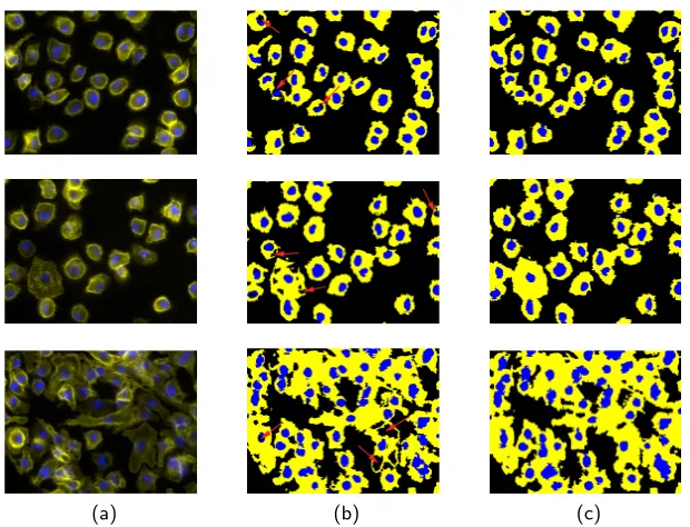
[image:12.612.152.462.240.477.2](a) (b) (c)
Fig. 5.Segmentation results for 3 samples from the image dataset. Column (a) shows real image samples. Columns (b) and (c) show segmentation results for GMM and the proposed method, respectively. Red arrows point to areas of the cell or the seeds that were not recognised by GMM, while the proposed algorithm segmented them correctly.
4
Conclusion
segmentation of cell surfaces and seeds in synthetic and real microscopy images. This study was focused on the application of the proposed method to image seg-mentation and three-wise constraints. However, the designed formulation can be straightforwardly used for more complex applications where more complicated constraints are required to be projected on the model.
Acknowledgments. This work was supported by MRC fellowship (MR/J009156/1)
and the Krebs Institute fellowship.
References
1. Arteta, C., Lempitsky, V., Noble, J.A., Zisserman, A.: Interactive object counting. In: European Conference on Computer Vision. pp. 504–518. Springer (2014) 2. Van den Bergh, M., Boix, X., Roig, G., Van Gool, L.: Seeds: Superpixels extracted
via energy-driven sampling. International Journal of Computer Vision 111(3), 298– 314 (2015)
3. Bishop, C.: Pattern Recognition and Machine Learning. Springer-Verlag New York (2006)
4. Boykov, Y., Veksler, O., Zabih, R.: Fast approximate energy minimization via graph cuts. IEEE Transactions on pattern analysis and machine intelligence 23(11), 1222–1239 (2001)
5. Chen, S.C., Zhao, T., Gordon, G.J., Murphy, R.F.: A novel graphical model ap-proach to segmenting cell images. In: Computational Intelligence and Bioinformat-ics and Computational Biology, 2006. CIBCB’06. 2006 IEEE Symposium on. pp. 1–8. IEEE (2006)
6. Girshick, R., Donahue, J., Darrell, T., Malik, J.: Rich feature hierarchies for ac-curate object detection and semantic segmentation. In: Proceedings of the IEEE conference on computer vision and pattern recognition. pp. 580–587 (2014) 7. Komodakis, N., Paragios, N., Tziritas, G.: Mrf energy minimization and beyond
via dual decomposition. IEEE transactions on pattern analysis and machine intel-ligence 33(3), 531–552 (2011)
8. Lafert´e, J.M., P´erez, P., Heitz, F.: Discrete markov image modeling and inference on the quadtree. IEEE Transactions on image processing 9(3), 390–404 (2000) 9. Ljosa, V., Sokolnicki, K.L., Carpenter, A.E.: Annotated high-throughput
mi-croscopy image sets for validation. Nat Methods 9(7), 637 (2012)
10. Pearl, J.: Probabilistic reasoning in intelligent systems: networks of plausible in-ference. Morgan Kaufmann (2014)
11. Rathke, F., Schmidt, S., Schn¨orr, C.: Probabilistic intra-retinal layer segmentation in 3-d oct images using global shape regularization. Medical image analysis 18(5), 781–794 (2014)