Teaching Excellence
Framework: Analysis of
highly skilled employment
outcomes
Research report
September 2016
2
Contents
List of tables 3
Acknowledgements 4
Executive Summary 5
Main report 8
Introduction 8
Review of existing literature 11
Methodology 13
Variables and Data 13
Choice of estimator 20
Goodness of Fit 21
Results 21
Application of results 26
Discussion 27
Conclusion 30
Annex A 31
Results from alternative models 31
Annex B 37
Binomial Generalised Linear Model 37
Annex C 39
Further analysis relating to REF score variable 39
3
List of tables
Table 1: Factors found to be statistically associated with highly skilled employment and
further study ... 7
Table 2: Number of HE institutions flagged significantly above or below benchmark, for employment and further study metric ... 10
Table 3: Number of HE institutions flagged significantly above or below benchmark, for highly skilled employment and further study (HSE) metric ... 10
Table 4: Description of Variables ... 15
Table 5: AIC values for each of the three fitted models ... 21
Table 6: Results of logit model ... 23
Table 7: Example of highly skilled employment or further study outcome ... 26
Table 8: Results of complementary log-log model ... 31
4
Acknowledgements
The authors would like to thank Pamela Meadows and Steve McIntosh for peer reviewing the report.
5
Executive Summary
A key motivation for many students entering higher education is the attainment of the skills and qualifications needed to realise their career ambitions, which often means being able to access higher skilled and professional occupations. The focus of this report is to consider what factors determine the likelihood of a student
finding such employment.
This analysis is timely as the Government is in the process of introducing a Teaching Excellence Framework (TEF) to provide greater recognition and reward for high quality teaching. At TEF’s heart will be an assessment made by an independent panel using a set of core performance metrics and further evidence on teaching quality submitted to it by providers. Following consultation, the Government has decided that one of the core metrics used should relate to the proportion of students who are in highly skilled employment or further study six months after graduation1.
As with other core metrics used in TEF, to ensure a fair assessment a provider’s
performance needs to be benchmarked against what might typically be expected in the sector, given its student and subject mix. Without this the panel cannot be confident that the performance it is seeing relates to the provider’s teaching quality as opposed to other things. An understanding, therefore, of the determining factors of highly skilled
employment outcomes is critical in establishing the appropriate factors to consider in such a benchmarking exercise.
Approach
To gain this understanding we used a binomial generalised linear model to test the relationship between the probability of being in highly skilled employment or further study six months after graduating, and a number of potential explanatory variables identified within existing literature and available from existing data sources.
Data on graduates’ employment and further study data was based on the Destinations of Learners in Higher Education (DLHE) survey. The definition of highly skilled employment is any occupation within categories 1-3 of the Standard Occupational Classification2. Other
key data was drawn from the Higher Education Statistics Agency (HESA) Student Record. We used Higher Education Funding Council for England (HEFCE) data on POLAR3 as a measure of social disadvantage.
1 See Teaching Excellence Framework – Year Two and Beyond for further detail
2 The category headings are: 1. Managers, directors and senior officials; 2. Professional occupations; 3.
Associate professionals and technical occupations. Further information can be found on the ONS website.
3 The participation of local areas (POLAR) classification groups areas across the UK based on the proportion
of the young population that participates in higher education (HE). Further information can be found on the
6
The sample population included in the analysis is the set of all UK-domiciled graduates from first degree courses in English higher education institutions in the 2011/12, 2012/13, and 2013/14 academic years who indicated their post-graduation activity when responding to the DLHE questionnaire, who have a known UCAS tariff, and with a known postcode and POLAR quintile.
Results
The Higher Education Statistics Agency publishes a set of UK performance indicators (UKPIs) which provide comparative data on the performance of higher education providers across several areas. One of the indicators measures employment and further study outcomes of graduates but there is no indicator for highly skilled employment and further study. Indicators are subject to a benchmarking methodology to aid fair and accurate comparisons.
Our analysis found that the factors used in the benchmarking for the UKPIs of
employment: gender, age, ethnicity, entry tariff (a proxy for prior attainment) and subject of study, were all statistically associated with the outcome of interest. However, it also found that region of domicile, social disadvantage (as measured by POLAR), disability and type of degree obtained were statistically significant factors.
We tested several proxy variables to capture the reputation of the institution attended. Variables based on the Research Excellence Framework score and the age of an institution were found to be statistically significant. However the scope of this analysis does not allow us to say whether these reputational factors are independent of teaching quality.
Conclusion
This report investigates what factors help to explain the proportion of students who go on to highly skilled employment or further study after graduating from a higher education institution. A number of factors are found to be statistically important, in addition to those currently used in the benchmarking approach for the UKPI measure of (all) employment and further study, as set out in table 1.
7
Table 1: Factors found to be statistically associated with highly skilled employment and further study
Factors used in employment UKPI Proxies for reputation Other factors
Gender REF score Region of domicile
Age Era of institution POLAR quintile
Ethnicity Degree type4 obtained
Entry tariff Disability
Subject of study
8
Main report
Introduction
A key motivation for many students entering higher education is the attainment of the skills and qualifications needed to realise their career ambitions, which often means being able to access higher skilled and professional occupations5. The focus of this report is to
consider what factors determine the likelihood of a student finding such employment.
This analysis is timely as the Government is in the process of introducing a Teaching Excellence Framework (TEF) to provide greater recognition and reward for high quality teaching6. The Government has introduced the TEF as a way of:
• Better informing students’ choices about what, where and how to study.
• Raising esteem for teaching.
• Recognising and rewarding excellent teaching.
• Better meeting the needs of employers, business, industry and the professions.
At TEF’s heart will be an assessment made by an independent panel using a set of core performance metrics and further evidence on teaching quality submitted to it by providers.
One metric will measure the proportion of graduates in any form of employment or further study six months after graduating. This metric follows the same definition as the existing UK Performance Indicator of employment. The Government’s technical consultation7
confirmed an appetite to include an additional metric that better captures the extent to which skills developed during higher education are used in the job. The Government has subsequently decided to include a core metric related to the proportion of students who are in highly skilled employment or further study six months after graduation.
The definition for this metric is the proportion of graduates employed within Standard Occupational Classification (SOC) 1-3, or in further study, six months after graduating, as measured by the Destination of Learners in Higher Education (DLHE) survey8. This will be
called the highly skilled employment (HSE) metric. Throughout this report the shorthand
5 See for example Purcell et al. (2008) and BIS (2012). 6 See the Government’s TEF Year Two Specification. 7Teaching Excellence Framework – Year Two and Beyond
8 Other definitions exist but assessment of those is out of the scope of this report (see methodology section
9
HSE denotes ‘being in highly skilled employment or further study six months after graduating’9.
Benchmarking
The Teaching Excellence Framework will not use raw scores to assess providers’
performance. This is because it is well established that such scores are influenced by the nature of their student intake and the mix of subjects they offer. As the purpose of TEF is to compare teaching quality and provide students with an indication of the added value they will receive from a provider, we need a method to control for these differences to provide more meaningful information about a provider’s performance and allow fairer comparisons across institutions.
This challenge is not new and TEF will follow an established methodology developed by HESA10. This involves adjusting the sector average for each HE provider to take into
account some of the factors which contribute to the differences between them. The resulting adjusted average is the ‘benchmark’, unique to each provider. The difference between the raw score and the benchmark provides a fairer and more meaningful measure of a provider’s performance.
The established criteria for inclusion in the benchmarks require factors under consideration to:
• Be associated with what is being measured.
• Vary significantly from one provider to another.
• Not be in the providers’ control, and so not be part of their performance.
This report tests the first of these criteria only.
The benchmark factors included in HESA’s UK Performance Indicator (UKPI) of
employment and further study outcomes are: subject of study, entry qualifications, age on entry, ethnicity and sex. The same factors are used in the benchmarking for the (all) employment and further study metric that will be used as part of the TEF assessment process. This report aims to determine whether these factors are also appropriate to use in the benchmarking for the highly skilled employment metric, and whether there are any further factors that should be considered.
9 Both the DLHE and the Key Information Set used for Unistats also employ a SOC 1-3 definition, and refer
to occupations within that category as ‘professional and managerial’. See HESA website for more detail.
10
TEF flags for highly skilled employment metric
To assist TEF panel assessments, where there is a significant difference between a provider’s raw score and benchmark for a particular metric, this will be ‘flagged’. The approach to flagging set out in the TEF Year 2 Specification11 was chosen to ensure
sufficient differentiation between those providers that are flagged positively (where the raw score is significantly greater than the benchmark), those that are flagged negatively (where the raw score is significantly lower than the benchmark) and those not flagged (where the raw score is not significantly different to the benchmark).
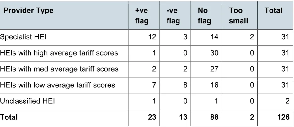
Tables 2 and 3 below reveal the results of an analysis of TEF data to assess the potential distribution of ‘flags’ across different higher education institutions (HEIs)12. In both tables,
[image:10.595.57.526.349.551.2]the benchmark factors used are those included in the UKPI for employment and further study, as described in the preceding section.
Table 2: Number of HE institutions flagged significantly above or below benchmark, for employment and further study metric
Provider Type +ve
flag -ve flag No flag Too small Total
Specialist HEI 12 3 14 2 31
HEIs with high average tariff scores 1 0 30 0 31
HEIs with med average tariff scores 2 2 27 0 31
HEIs with low average tariff scores 7 8 16 0 31
Unclassified HEI 1 0 1 0 2
[image:10.595.58.522.612.681.2]Total 23 13 88 2 126
Table 3: Number of HE institutions flagged significantly above or below benchmark, for highly skilled employment and further study (HSE) metric
Provider Type +ve
flag -ve flag No flag Too small Total
Specialist HEI 18 6 5 2 31
11 The TEF Year Two Specification
12 The TEF Year Two Specification proposes that a metric is flagged positive if it is 2 percentage points and
11
Provider Type +ve
flag -ve flag No flag Too small Total
HEIs with high average tariff scores 19 2 10 0 31
HEIs with med average tariff scores 8 16 7 0 31
HEIs with low average tariff scores 5 19 7 0 31
Unclassified HEI 1 0 1 0 2
Total 51 43 30 2 126
Tables 2 and 3 present indicative significance flag results based on students graduating from full-time undergraduate programmes at English HEIs across the most recent three years of data (academic years 2011-12, 2012-13 and 2013-14) available at the time of the analysis, based on teaching institution in their final year. Figures are based on unverified analysis for TEF development purposes.
HEIs are split into specialist, unclassified and three equally sized groups based on entry tariff requirements.
The tables show that many more providers are flagged as being significantly above or below their benchmarks for the HSE metric than for the overall employment metric – 94 against 36. Furthermore, high tariff institutions tend to perform much better against this metric than medium and low tariff institutions.
This may be a valid reflection of better teaching quality in these types of provider. But this effect is not apparent in other metrics. An alternative theory is that employers recruit graduates to high-skilled jobs based on the reputation or prestige of the provider they attended. As TEF seeks to measure teaching quality, it would be undesirable to include a metric that is driven by reputation where that does not reflect the quality of teaching. A second alternative theory is that social advantage – associated with prior attainment and hence attendance at higher tariff institutions – confers an advantage in the highly skilled graduate jobs market.
This report explores how different variables, including measures of institutional reputation and social disadvantage, affect the probability of a student entering highly skilled
employment or full-time further study.
Review of existing literature
The key question which this report focuses on is: what determines high skill employment (HSE)?
12
literature review highlights that employment outcomes were considered the most important factor by students when choosing a Higher Education establishment in 2015 (Higher Education Policy Institute, 2016). The review also identifies, however, that some students recognise that employment outcomes will be influenced by other factors. This is consistent with findings from the international literature.
The existing literature points to a range of factors in addition to teaching quality which are considered to influence highly skilled employment outcomes for graduates, including:
• The macro-economic performance of the UK as a whole and the regions which segment it - which in turn influence labour market trends. Basnett & Sen (2013) find that economic growth is positively associated with job creation. For every 1
percentage point of additional GDP growth, total employment has grown between 0.3 and 0.38 percentage points between 1991 and 2003. Whilst this study focuses on total employment we also expect the relationship to remain for HSE growth.
• The individual characteristics, skill and ability levels of students, including:
• Age, gender, and ethnicity. Ramsey, 2008, explores returns with factors such as age, gender, social class, institution type, and geographic location.
Tackey et al, 2011 uses this research to discern that full-time degree graduates from all minority ethnic groups have higher initial unemployment rates than white graduates.
• Subject choice and degree classifications. De Vries, 2014, shows that there are large variations in outcomes for graduates depending on their university and degree subject. Additionally many graduate schemes have a minimum grade requirement which may result in skewing of the HSE data between the grades 2:1 and 2:2.
• Whether they attended state or private school. Macmillan, Tyler, Vignoles, 2013, find for example that privately educated graduates are a third more likely to enter into high status occupations than state educated graduates from similarly affluent families and neighbourhoods.
• Socio-economic class and the role of networks which includes family and neighbourhood experiences in accessing highly skilled employment. Purcell, 2012, found that socio-economic background appeared to have the closest relationship with whether a respondent had taken part in extra-curricular activities while in HE or been an office holder. It was found that those students who had extra-curricular or office-holder experiences in HE were more likely to gain highly skilled employment after graduating.
13
• Undertaking paid/unpaid work and other qualifications while at university such as internships and placements, or in the six months immediately after; and
• Focusing job searches exclusively on HSE and making the majority of applications while still studying; and having a career plan upon leaving university.
• Employers behaviour (Connor, Hirsh and Barber, 2003) in targeting specific HEIs for their recruitment efforts for reasons including:
• An institution’s reputation or academic rigour – this appeared to be a very common practice amongst certain recruiters, for example, for those with fast-track, high potential schemes,
• Geographical proximity,
• Previous positive track record in providing high calibre candidates, and
• A need to focus resources and limit the number of potential applicants.
These literature review findings are consistent with the aim of this report - to build on the existing literature and collate the identified factors, including reputational and social effects, which influence highly skilled employment outcomes. Where possible we have included data on the factors suggested from the literature in our database, as described in the following section.
Methodology
This section describes the dataset used, the variables tested, and the model specifications assessed.
Variables and Data
Level of Analysis
14
Population covered
The sample population included in the analysis is the set of all UK-domiciled graduates from first degree courses in English HEIs in the 2011/12, 2012/13, and 2013/14 academic years who indicated their post-graduation activity when responding to the DLHE
questionnaire, who have a known UCAS tariff, and with a known postcode and POLAR quintile.
As a result of data availability, the sample population included in this analysis is not entirely consistent with the population in scope for TEF. In particular, further education colleges and alternative providers are not included. Nor are graduates from Scottish, Welsh or Northern Irish providers, nor undergraduates from level 4 or 5 courses.
Response of interest
The dependent variable, or response of interest, is whether or not the student entered highly skilled employment (defined as SOC categories 1-3)13, or entered further study, six
months after graduating. This is a standard way of defining this type of employment – for instance ‘professional and managerial job’ graduate outcomes recorded on Unistats follows the same definition14. This is also the measure and definition of highly skilled
employment set out in the TEF specification.
The appropriateness of that definition is not assessed further in this report. However we acknowledge that some providers may perform less well against this measure for reasons unrelated to teaching quality. For instance, graduates from arts or drama degrees from specialist HEIs may not consider a SOC 1-3 occupation to be a desirable outcome. These sorts of differences should be controlled for through the variables tested, such as subject of study.
Response rates for the DLHE over the years included in the analysis were 78-79%. It is possible that non-response is (negatively) correlated with the outcome of interest. Results must therefore be treated with a degree of caution as no adjustment was made to correct for non-response bias. The Office for National Statistics recently reviewed the data
sources used for TEF and recommended that an adjustment for non-response should be made15. The DLHE itself is currently subject to a review and consultation which could lead
to its alteration or replacement16. It is therefore possible that future iterations of the data
will not suffer from this shortcoming.
13 The category headings are: 1. Managers, directors and senior officials; 2. Professional occupations; 3.
Associate professionals and technical occupations. Further information can be found on the ONS website.
14 See Unistats website.
15
It is also worth noting that development of the Longitudinal Employment Outcomes (LEO) dataset may offer an alternative or complementary measure of highly skilled employment in the future17.
Variables considered in the analysis
The factors we chose to test came from several sources. We wanted to test those factors already used in the benchmarking process for the existing UK Performance Indicator of employment: subject of study, entry qualifications, age on entry, ethnicity, and sex.
We also wanted to test factors that reflected the reputation or prestige of institutions. In the absence of data that measures this directly, we created and tested three potential
reputation variables: Russell Group membership, Research Excellence Framework score and institution age. Details of these are provided below.
Finally we tested several other factors which were considered likely to have an impact on highly skilled employment and to vary by provider, based upon a study of the literature, the views of the BIS-HEFCE expert steering group and feedback from external peer review. These included regional factors and measures of social disadvantage.
Some variables were not included in the dataset, either because appropriate data did not exist, or because after consideration they were deemed not to be relevant. For example, data could not be obtained in the time available on level of degree or on whether students attended state or private school. Unemployment rates were considered but not included because the academic year and regional variables were expected to pick up the relevant economic and labour market trends.
[image:15.595.49.550.583.726.2]Table 4 provides a description of all the variables identified and their rationale for inclusion. After testing, not all variables were included in the final estimator (see further explanation on page 20).
Table 4: Description of Variables
Variable Description Variable type Rationale Skilled job flag This is a flag that
denotes whether the student was in a job falling within SOC codes 1 to 3 or in full-time further study 6 months after graduation
Binary: True, False This is the dependent variable
16
Variable Description Variable type Rationale Academic
Year
This is a marker that indicates the academic year of graduation
Categorical: 2011/12, 2012/13, 2013/14
Students who graduated in different years may be exposed to different economic conditions and thus have different probabilities of getting a skilled job
HE Institution The Higher Education Institution from which the student graduated
Categorical: 119 HEIs Any effects not captured by any of the other variables can be described as "institutional effects", including the teaching quality of the institution
Sex The sex of the student Categorical: Male, Female, Other Baseline: Male
There are observable differences in employment outcomes by sex.
Age The age of the student at August 31st at the academic year of graduation
Continuous: range:
18-81 There are observable differences in employment outcomes by age.
Ethnicity The ethnicity of the student
Categorical: White, Black, Asian, Other, Unknown
Baseline: White
There are observable differences in employment outcomes by ethnicity.
Disability Whether or not the student has a disability and, if so, what type
Categorical: 12
categories (see Table 6) Baseline: No disability
There are observable differences in employment outcomes by disability.
Institution
Region The region in which the HEI is located Categorical: 9 categories (see Table 6) Baseline: North East
Students graduating from HEIs in regions with relatively high employment rates should have a higher probability of getting a skilled job
Domicile
Region The region in which the student is domiciled prior to studying.
Categorical: 9 categories (see Table 6)
Baseline: North East
17
Variable Description Variable type Rationale Employment
Region
The region of post-graduation employment
Categorical: 9 categories (see Table 6)
Baseline: North East
Different regions may have different availabilities of skilled jobs
Polar Quintile i The POLAR quintile of
the student's domicile (a measure of HE
participation, by post code)
Categorical: 1, 2, 3, 4, 5 Socially disadvantaged students from areas of lower HE participation may have different employment outcomes
Subject of study
The subject which the student studied in the university, recorded as a set of percentages for students whose course encompasses two or more subjects
Categorical: 19
categories (see Table 6) Baseline: Combined Honours
Different subjects offer very different access to skilled jobs after graduation
Mode The student's mode of study
Binary: Full-time, Part-time
Employment outcomes may differ between full-time and part-time graduates
Degree
obtained A marker for the type of degree the student graduated with
Categorical: Honours First Degree, Ordinary First Degree, Master’s Degree
Baseline; Honours First Degree
Employment outcomes may differ between graduates of Masters Degrees, Honours First Degrees, and Ordinary First Degrees
Entry Tariff ii The UCAS tariff of the student at the point of entry to their course
Continuous: range: 5-1,600; 1st quartile: 260,
median: 340, 3rd quartile:
420
Students with greater latent ability and motivation may be more likely to have higher prior attainment (UCAS tariff) and be more likely to get skilled jobs, irrespective of teaching quality at their university Average Tariff The average UCAS
tariff of all graduates from the HEI
Continuous: range: 125-575
18
Variable Description Variable type Rationale Russell Group
iii A flag that indicates whether the HEI is part
of the Russell Group
Binary: True, False Employers may be more likely to make skilled jobs available to graduates of Russell Group universities which may act as a signal of quality
Research
Excellence iv A numeric score that summarizes an
institution's research excellence
Continuous: range: 1.29-3.49
Employers are more likely to make skilled jobs available to graduates of prestigious HEIs and prestige may be correlated with research excellence Institution Age
v A marker that splits HEIs into four
categories representing differing lengths of establishment
Categorical: Ancient (established pre 1800), Red Brick (1800-1960), Plate Glass (1960-1992), or post-92 (established post 1992) Baseline: Ancient University
Employers are more likely to make skilled jobs available to graduates of HEIs with an extensive historical reputation which may act as a signal of quality
All data was sourced from the HESA student record and HESA DLHE record unless otherwise specified.
i Sourced from HEFCE data.
ii Note that this measure differs slightly from the UKPI measure used in existing benchmarking. We use the
raw UCAS tariff only. The UKPI method employs an eleven level categorisation based on overall tariff, A-level or Scottish Higher grade combinations, and other measures.
iii Sourced from Russell Group website.
iv Sourced from Times Higher Education website and REF data. v Based on internet research and official university websites.
Baseline Levels
Many of the variables included in our analysis are categorical measures and require a reference or baseline level to be selected, against which other levels within that particular variable are measured. Variables fitted are effectively making a comparison with the baseline characteristics, for example the marginal impact on the likelihood of a HSE
outcome for a female student compared to a male student. Variables which are continuous do not require a baseline. The baseline levels in the fitted estimators are described in table 4.
19
Reputation variables
A University’s reputation or prestige might be an important influence on how employers regard the quality of graduates (at this point we do not consider whether or not reputation provides an accurate signal of teaching quality, only whether it has an effect on highly skilled employment and further study outcomes). Reputation and prestige are, however, rather subjective and ill-defined concepts. It is therefore unsurprising that no single piece of data exists to measure them directly. Nonetheless we felt this was potentially an important driver of HSE outcomes and therefore considered a number of proxy variables that could reflect reputation effects.
We thought that university league tables, although not formally recognised by the
Government, were one major driver of perceptions of reputation. The most well-known of these are based upon measures of teaching and reputation. Since the purpose of this study is to identify factors that determine HSE but are not related to teaching quality, we needed to remove the teaching element. We settled on the method employed by Times Higher Education to convert Research Excellence Framework (REF) scores into a grade point average. This method aggregates the units of assessment for each institution based on the number of full time equivalent staff assigned to each18.
We also thought that membership of widely recognised groups could affect reputation. There were numerous options for splitting HEIs into different groups. We settled on one simple measure that separated Russell Group universities from all others on the basis that the Russell Group is the best known university grouping.
History and length of establishment was another route to reputation that we considered. We created a variable based directly on the length of time an HEI had been established, grouped into the four commonly employed denominations of Ancient, Red Brick, Plate Glass and Post-92 Universities.
The average tariff variable (the average of all students’ individual tariffs at a particular institution) can also be considered a proxy for reputation. Demand from prospective students is likely to be linked to reputation, and institutions facing high demand are more likely to impose higher tariffs to deal with that. There is therefore a direct link between tariff and reputation.
Interaction terms
Many of the variables in Table 4 are interrelated. It is therefore possible that interaction terms – in which two or more variables are combined – would better approximate the true scale of impact than individually considered variables. However the primary aim of this study was to identify which factors have a statistically significant effect on HSE and should
20
therefore be considered as benchmark factors. Identifying the precise magnitude of that effect was of secondary importance.
For reasons of simplicity and timeliness, we therefore only considered a limited number of interaction terms. These have not been included in the final specification. In some cases, assessment of interaction terms was problematic. For example, an interaction between ethnicity and disability was assessed. Given that the large majority of students in the dataset are white, the only statistically significant interaction terms were with various disabilities and white students. This tells us very little about any additional effect between ethnicity of students and disabilities in combination.
Excluded variables
Some of the variables described in table 4 were excluded from the final specification. We systematically tested the appropriateness of including variables, based on consideration of a number of factors including multicollinearity, endogeneity and over-fitting.
The nature of this dataset makes some degree of correlation between explanatory variables inevitable. Such ‘multicollinearity’ can be direct (for example, subject studied might be linked to gender) or the result of a common unobserved factor affecting two or more explanatory variables. Where multicollinearity is high, standard errors tend to be artificially high and coefficients can be unstable. Common practice is to remove one or more of the affected variables from the model. Separate modelling found that the variables which measure Russell Group membership and average tariff of an institution were highly correlated with the variable which measures the era of the institution. We took the
judgement that they should therefore be excluded from the final specification.
The validity of results can be undermined by ‘over-fitting’ – the inclusion of too many variables in comparison to the size of the dataset. This ruled out the inclusion of a dummy variable for each higher education institution. In addition, the variables for academic year and mode of study were excluded because their inclusion did not affect the size or level of significance of the other included variables and they are not in themselves the focus of the study (TEF assessments will be made independently on different academic years and different modes of study).
Choice of estimator
The nature of the dataset, in particular the binomial nature of the response variable of interest, meant that using a binomial generalised linear model was appropriate. There were three estimators which we deemed suitable and each of these was fitted to the data. The three estimators fitted are associated with one of three link functions:
21
• Probability Unit (Probit).
• Logit.
The link function is a means of transforming the fitted data so that the response falls within the interval [0,1], which is necessary given that the response is a binomial probability. A further detailed explanation of the binomial generalised linear model approach can be found in annex B.
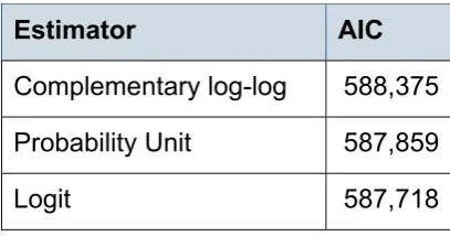
Goodness of Fit
[image:21.595.195.399.330.437.2]Table 5 summarises the Akaike Information Criterion (AIC) for the three fitted estimators. The AIC is a measure of how well an estimator fits a dataset, while adjusting for the ability of that estimator to fit any dataset, no matter how complex. The aim is to minimise the AIC.
Table 5: AIC values for each of the three fitted models
Estimator AIC
Complementary log-log 588,375
Probability Unit 587,859
Logit 587,718
It can be seen from the results presented in table 6, and tables 8 and 9 in annex A, that the parameter estimates are not too dissimilar and that the same variables are statistically significant in each. It is thus natural to choose the estimator which has the lowest value of the AIC, as this is regarded as having the best fit.
Results
This section describes the results of the analysis, concentrating on the estimator found to have the best fit. Results for the other estimators tested are set out in annex A. A guide to interpreting the results is set out below.
Estimate
22
The coefficient tells us whether the probability increases or reduces, but because the model is complex we cannot use the coefficient on its own to estimate the size of the change in probability. Instead we must take the exponential of the coefficient. In the example above the exponential of 0.743 is 2.012, implying that the odds of being in highly skilled employment or further study are more than twice as high for a graduate of computer science as they are for a graduate of a combined honours degree.
As a guide, coefficients of 0.5 or lower increase the odds of HSE by up to 65%, and coefficients of 0.1 or lower only increase the odds of HSE by up to 10%. The opposite applies for negative coefficients. The application of results section on pages 26-27 provides a fuller illustration of the effect of the coefficients.
In table 6, within each broad variable grouping, terms are ordered by coefficient estimate, from highest to lowest.
P-value
The ‘p-value’ represents the probability (between 0 and 1) that any association found between a variable and HSE (in relation to the baseline level for categorical variables) is just the result of chance, rather than reflecting a true relationship. Thus, a large p-value indicates a high probability that the estimated association is due to chance. On the other hand, a small p-value increases our confidence that the estimated association is due to a true relationship existing between the variables.
Significance
The p-value allows the statistical significance of an association between variables and HSE to be determined. In this report we use 0.05 as the critical level. In other words, all associations for which the p-value is smaller than 0.05 are defined as statistically
significant. We also distinguish different levels of statistical significance because the smaller the p-value, the more confident we can be in the validity of the association found.
The significance column in table 6 provides a visual representation of the p-value and the associated level of statistical significance. The relevant levels of significance are:
‘*’ = p-value of less than 0.05 (5% level of statistical significance)
‘**’ = p-value of less than 0.01 (1% level of statistical significance)
‘***’ = p-value of less than 0.001 (0.1% level of statistical significance)
23
Frequency
This information shows the number of graduates who exist within the dataset for each term included in the final specification.
[image:23.595.53.527.222.771.2]Table 6 shows the results of the binomial generalised linear model fit to the dataset with the logit link function.
Table 6: Results of logit model
Variable Term Estimate p-value Significance Frequency
Intercept Parameter -1.760 0.000 ***
Gender Baseline: Male 212,144
Female -0.143 0.000 *** 256,066
Age Age 0.046 0.000 ***
Ethnicity Baseline: White 377,980
Other -0.121 0.000 *** 20,856
Unknown -0.213 0.000 *** 3,632
Black -0.265 0.000 *** 19,279
Asian -0.284 0.000 *** 55,486
Subject Baseline: Combined Honours
1,795
Medicine 3.909 0.000 *** 10,725
Veterinary 1.561 0.000 *** 1,083
Medicine (allied) 1.391 0.000 *** 30,995
Architecture 1.038 0.000 *** 9,770
Education 1.033 0.000 *** 20,880
Computer Science 0.743 0.000 *** 16,497
Engineering 0.583 0.000 *** 23,484
Mathematical
Sciences
0.327 0.000 *** 12,679
24
Variable Term Estimate p-value Significance Frequency
Law 0.269 0.000 *** 21,046
Physical Sciences 0.034 0.517 26,212
Social Studies 0.034 0.506 49,070
Arts -0.033 0.519 56,060
Biological Sciences -0.046 0.358 56,471
Communications -0.070 0.179 17,022
Languages -0.106 0.038 * 36,974
Agriculture -0.194 0.001 ** 3,693
History -0.240 0.000 *** 27,811
Disability Baseline: No
Disability 425,161
Unknown 0.303 0.065 224
Learning Difficulty 0.050 0.000 *** 30,979
Hearing Impairment -0.037 0.578 1,038
Other -0.037 0.257 4,403
Visual Impairment -0.089 0.291 642
Health Condition -0.108 0.000 *** 5,071
Physical Impairment -0.161 0.004 ** 1,395
Two or More
Conditions
-0.172 0.000 *** 2,200
Mental Health
Condition
-0.221 0.000 *** 4,853
Autistic Spectrum
Disorder -0.466 0.000 *** 1,265
Domicile Baseline: North East 18,799
East of England 0.229 0.000 *** 53,496
25
Variable Term Estimate p-value Significance Frequency
South East 0.209 0.000 *** 82,410
West Midlands 0.188 0.000 *** 46,361
Scotland 0.179 0.000 *** 2,504
South West 0.167 0.000 *** 39,978
Yorkshire and the
Humber
0.095 0.000 *** 40,820
Wales 0.094 0.001 *** 9,521
London 0.028 0.120 80,012
North West -0.004 0.831 60,447
Northern Ireland -0.019 0.584 4,855
Polar quintile
5th (highest quintile) 0.624 0.000 *** 160,173
4th 0.468 0.000 *** 114,875
3rd 0.312 0.000 *** 91,295
2nd 0.156 0.000 *** 67,524
1st (lowest quintile) 0 0.000 *** 43,366
Entry tariff Individual student tariff
0.002 0.000 ***
Degree Obtained
Baseline: Honours Undergraduate Degree
448,735
Master’s degree 0.605 0.000 *** 24,757
Ordinary
Undergraduate degree
-0.520 0.000 *** 3,741
Research
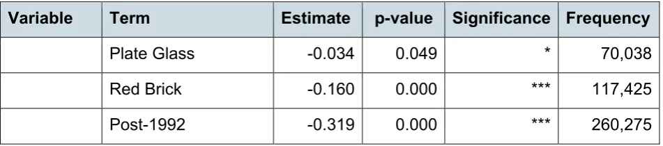
Excellence Research excellence score 0.209 0.000 ***
Era of
University Baseline: Ancient University
26
Variable Term Estimate p-value Significance Frequency
Plate Glass -0.034 0.049 * 70,038
Red Brick -0.160 0.000 *** 117,425
Post-1992 -0.319 0.000 *** 260,275
In terms of existing benchmark factors used in the employment and further study UKPI, Table 6 confirms that gender, age, ethnicity, entry tariff and subject studied all have a statistically significant impact on HSE. Specifically a graduate is more likely to be in highly skilled employment or further study if they are male, older, white, have better school results (higher entry tariff) and studied certain subjects such as medicine or business.
The results also suggest other factors are important: region of domicile, social
disadvantage (measured by POLAR), disability19 and type of degree obtained. Specifically
a graduate is more likely to be in highly skilled employment or further study if they lived in certain regions such as the South East or East Midlands before studying, lived in an area with a higher level of HE participation (higher POLAR quintile) before studying and
graduated with a higher level of degree.
Finally, the reputation of the provider appears to have a significant impact on HSE. A graduate is more likely to be in highly skilled employment or further study if they attended an institution with a higher research excellence score or if they attended an older institution (though attending a Plate Glass era institution leads to better outcomes than attending a Red Brick era institution).
Application of results
This section provides an illustration of how the results can be used to construct the probability of a graduate with certain characteristics obtaining a highly skilled job or entering further study.
[image:26.595.51.527.84.189.2]The example set out in Table 7 draws in general upon the modal (most common) value or category for each variable.
Table 7: Example of highly skilled employment or further study outcome
Variable Graduate A Coefficient
Gender Female -0.143
19 Interestingly, the analysis suggests that, unlike all the other disability categories, having a learning
27
Variable Graduate A Coefficient
Age 22 years old 0.046
Ethnicity White 0
Subject studied Business 0.285
Disability None 0
Domicile South East 0.209
POLAR quintile 5th (top) 0.624
Entry tariff 340 0.002
Degree obtained Honours undergraduate 0
Institution’s REF score 2.75 0.209
Era of institution Post-92 -0.319
To find the overall estimate, we use equation 3 from Annex B, remembering to include the intercept of -1.76.
The estimated odds of being in highly skilled employment or further study six months after graduation are equal to the exponential of the sum of coefficients from Table 7:
𝑂𝑂𝑂𝑂1 = exp{−1.76 − 0.143 + 0.046 ∗ 22 + 0.285 + 0.209 + 0.624 + 0.002 ∗ 340 + 0.209
∗ 2.75 − 0.319}
𝑂𝑂𝑂𝑂1 = 3.20
This indicates that the odds of graduate A being in highly skilled employment or further study six months after graduation are a little over 3 to 1.
To convert the odds into a probability,𝜃1, the following transformation is made:
𝜃1 = 1 + exp {3.20}exp {3.20}
𝜃1 = 0.762
This indicates that the probability of graduate A being in highly skilled employment or further study six months after graduation are 0.762 or 76.2%.
Discussion
28
benchmarking approach for the highly skilled employment metric in TEF. However, as explained in the introduction, statistical association is only one condition a benchmarking factor needs to meet. Other conditions include:
• The factor must vary between providers.
• The factor must not be within the control of the provider.
• The factor must not be related to teaching quality.
The rest of this section covers some of the other analytical issues that might need to feed into this thinking, focusing on the factors not currently employed by the UK Performance Indicators – reputation, social disadvantage and regions. It also suggests some areas for further work.
Reputation
The positive coefficients for research excellence score (REF score) and era of university can be interpreted in more than one way. If we believe that these variables are good, reliable proxies for reputation then the results support the theory that employment is driven by reputation, and that we should consider controlling for this through benchmarking.
However, other factors need to be considered before incorporating it into the
benchmarking methodology. Starting with the REF variable, its positive coefficient could be interpreted as evidence in support of the theory that excellent research fosters or facilitates excellent teaching, which then leads to better employment outcomes. If so, this would seem to rule REF score out as a potential benchmark factor because we must avoid controlling for any factor that is linked to teaching when considering applicability to TEF.
Alternatively, it might be argued that while research rating does help to drive reputation, employers are focusing on this not because it has any reliable link to teaching quality, but because the information is more readily available. If this were true then there would
nevertheless be a different risk to including REF as a benchmark factor for TEF because it would create a tension between the two programmes. A provider that improved its REF score would be faced with a higher benchmark, and might therefore receive a lower TEF award even with no change to its teaching quality. This could create a disincentive for institutions to invest in research capacity, which would be an undesirable outcome.
The era of institution variable is not a measure of the research ability of current staff, so does not suffer from the two issues described above. However there is a third issue which affects both the REF and era of institution variables. Reputation influences not only
students, but academic staff too. If the best academics are attracted to the institutions with the highest reputation, then good teaching could be correlated with measures of
29
On the other hand, if the keenest researchers are attracted to the most reputable institutions, but are bad teachers, poor teaching could be correlated with measures of reputation. Either way there is a potential link between measures of reputation and
teaching which means it may not be appropriate to include them as benchmark factors for HSE. See annex C for a summary of further analytical investigation into this particular issue.
A further argument related to era of institution is that older universities have had time to build up and perfect a method of teaching unique to them and that, therefore, era could be a measure of teaching quality as well as reputation.
Social Disadvantage
The high degree of significance demonstrated for the POLAR variable suggests that a measure of social disadvantage should be considered as a benchmark factor for the HSE metric.
This analysis has focused on the use of POLAR, which is perhaps the most widely accepted measure of social disadvantage in a higher education context. There are,
however, other measures of social disadvantage – with their own particular pros and cons – that could be considered in more depth in the longer term. These include the Social Mobility Index, the Index of Multiple Deprivation, and Socio-Economic Classifications.
Regional variables
We initially considered three regional variables. Employment region was excluded from the final specification since it was judged to be more of a co-factor of HSE rather than a causal factor. Due to the high degree of correlation between institution region and domicile region, we deemed it appropriate to exclude one from the final specification. Analysis of DLHE data20 suggests that more graduates work in their region of domicile than their region of
study. Therefore we included domicile region in the final model and it was found to be a statistically significant factor.
However, suitability of a regional indicator for inclusion as a benchmark factor depends upon additional considerations. There are two potential drawbacks that should be
considered in particular. Firstly, regions are an imperfect, blunt way of accounting for local labour market conditions. Employment rates, for instance, can vary significantly within regions, particularly between large cities and rural areas. Therefore effects aggregated to the regional level may not be representative of the prevailing employment prospects a graduate faces in the specific area they live or study in.
Secondly, the relatively large number of categories of region (12) may reduce the effectiveness of the benchmarking. The more benchmark categories we include, the
30
smaller become the groups of comparable students. This makes comparison of institutions’ performance less meaningful.
Conclusion
We used a binomial generalised linear model to test the relationship between the probability of being in highly skilled employment or further study six months after
graduating, and a number of explanatory variables. We found that the factors used in the benchmarking for the employment UK Performance Indicator: gender, age, ethnicity, entry tariff and subject of study, were all statistically significant drivers of highly skilled
employment and further study. We also found that region of domicile, POLAR quintile (a measure of HE participation in a local area), disability and type of degree obtained were statistically significant factors.
We tested three proxy variables for the reputation of the provider attended. The variable for Russell Group membership was excluded from the final model due to correlation with several other explanatory variables. However variables based on the Research Excellence Framework and age of institution were found to be statistically significant.
31
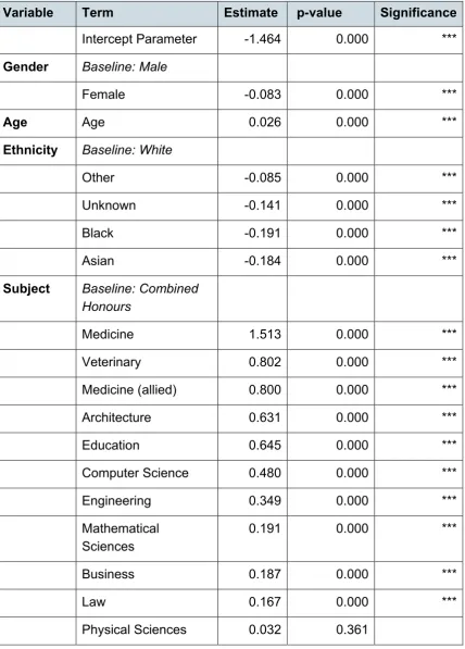
Annex A
[image:31.595.54.483.179.777.2]Results from alternative models
Table 8: Results of complementary log-log model
Variable Term Estimate p-value Significance
Intercept Parameter -1.464 0.000 ***
Gender Baseline: Male
Female -0.083 0.000 ***
Age Age 0.026 0.000 ***
Ethnicity Baseline: White
Other -0.085 0.000 ***
Unknown -0.141 0.000 ***
Black -0.191 0.000 ***
Asian -0.184 0.000 ***
Subject Baseline: Combined Honours
Medicine 1.513 0.000 ***
Veterinary 0.802 0.000 ***
Medicine (allied) 0.800 0.000 ***
Architecture 0.631 0.000 ***
Education 0.645 0.000 ***
Computer Science 0.480 0.000 ***
Engineering 0.349 0.000 ***
Mathematical Sciences
0.191 0.000 ***
Business 0.187 0.000 ***
Law 0.167 0.000 ***
32
Variable Term Estimate p-value Significance
Social Studies 0.024 0.474
Arts -0.037 0.274
Biological Sciences -0.045 0.185
Communications -0.071 0.044 *
Languages -0.062 0.070
Agriculture -0.143 0.001 ***
History -0.150 0.000 ***
Disability Baseline: No Disability
Unknown 0.171 0.059
Learning Difficulty 0.028 0.001 ***
Hearing Impairment -0.022 0.617
Other -0.028 0.179
Visual Impairment -0.076 0.169
Health Condition -0.068 0.001 ***
Physical Impairment -0.112 0.003 **
Two or More Conditions
-0.122 0.000 ***
Mental Health Condition
-0.152 0.000 ***
Autistic Spectrum Disorder
-0.330 0.000 ***
Domicile Baseline: North East
East of England 0.138 0.000 ***
East Midlands 0.132 0.000 ***
South East 0.125 0.000 ***
West Midlands 0.113 0.000 ***
33
Variable Term Estimate p-value Significance
South West 0.100 0.000 ***
Yorkshire and the Humber
0.055 0.000 ***
Wales 0.055 0.001 **
London 0.012 0.327
North West -0.003 0.776
Northern Ireland -0.010 0.669
Polar
quintile 5
th (highest quintile) 0.392 0.000 ***
4th 0.294 0.000 ***
3rd 0.196 0.000 ***
2nd 0.098 0.000 ***
1st (lowest quintile) 0.000 0.000 ***
Entry Tariff
Tariff 0.002 0.000 ***
Degree
Obtained Baseline: Honours Undergraduate Degree
Master’s degree 0.315 0.000 ***
Ordinary
Undergraduate degree
-0.336 0.000 ***
Research
Excellence Research excellence score
0.144 0.000 ***
Era of University
Baseline: Ancient University
Plate Glass 0.031 0.002 **
Red Brick -0.059 0.000 ***
34
Table 9: Results of probit model
Variable Term Estimate Pr(>|z|) Significance
Intercept Parameter -1.069 0.000 ***
Gender Baseline: Male
Female -0.086 0.000 ***
Age Age 0.027 0.000 ***
Ethnicity Baseline: White
Other -0.076 0.000 ***
Unknown -0.131 0.000 ***
Black -0.164 0.000 ***
Asian -0.174 0.000 ***
Subject Baseline: Combined Honours
Medicine 1.936 0.000 ***
Veterinary 0.897 0.000 ***
Medicine (allied) 0.830 0.000 ***
Architecture 0.631 0.000 ***
Education 0.632 0.000 ***
Computer Science 0.458 0.000 ***
Engineering 0.352 0.000 ***
Mathematical Sciences
0.197 0.000 ***
Business 0.175 0.000 ***
Law 0.164 0.000 ***
Physical Sciences 0.023 0.473
Social Studies 0.021 0.502
Arts -0.023 0.464
35
Variable Term Estimate Pr(>|z|) Significance
Communications -0.048 0.142
Languages -0.063 0.045 *
Agriculture -0.122 0.001 **
History -0.147 0.000 ***
Disability Baseline: No Disability
Unknown 0.182 0.060
Learning Difficulty 0.030 0.000 ***
Hearing Impairment -0.024 0.555
Other -0.023 0.243
Visual Impairment -0.059 0.255
Health Condition -0.065 0.000 ***
Physical Impairment -0.100 0.004 **
Two or More Conditions
-0.107 0.000 ***
Mental Health
Condition -0.137 0.000 ***
Autistic Spectrum Disorder
-0.289 0.000 ***
Domicile Baseline: North East
East of England 0.138 0.000 ***
East Midlands 0.133 0.000 ***
South East 0.126 0.000 ***
West Midlands 0.114 0.000 ***
Scotland 0.102 0.000 ***
South West 0.101 0.000 ***
Yorkshire and the Humber
36
Variable Term Estimate Pr(>|z|) Significance
Wales 0.057 0.001 ***
London 0.015 0.165
North West -0.003 0.814
Northern Ireland -0.011 0.608
Polar quintile
5th (highest quintile) 0.38 0.000 ***
4th 0.285 0.000 ***
3rd 0.19 0.000 ***
2nd 0.095 0.000 ***
1st (lowest quintile) 0.095 0.000 ***
Entry Tariff
Tariff 0.002 0.000 ***
Degree
Obtained Baseline: Honours Undergraduate Degree
Master’s degree 0.352 0.000 ***
Ordinary
Undergraduate degree
-0.313 0.000 ***
Research Excellence
Research excellence score
0.130 0.000 ***
Era of University
Baseline: Ancient University
Plate Glass -0.006 0.563
Red Brick -0.086 0.000 ***
37
Annex B
Binomial Generalised Linear Model
All generalised linear models feature the following three components (Dobson and Barnett, 2008):
1. Random component: Response variables 𝜃1, … , 𝜃𝑛, independently identically
distributed according to a distribution belonging to the exponential family of distributions, where 𝑛 is the number of observations for a given dataset.
2. Systematic component: A linear predictor of 𝑘 covariates and 𝑘 + 1 parameters:
𝜂𝑖 = 𝛼 + 𝛽1𝑋𝑖1+ 𝛽2𝑋𝑖2+ ⋯ + 𝛽𝑘𝑋𝑖𝑘 ,
where 𝑋𝑖𝑖 is the 𝑗th covariate of the 𝑖th subject, with 𝛽𝑖 the coefficient of the 𝑗th
covariate and 𝛼 the intercept parameter.
3. Link function: A monotone link function 𝑔, such that:
𝑔(𝜇𝑖) = 𝜂𝑖 ,
where 𝜇𝑖 = 𝐸(𝜃𝑖).
The response variable of interest for a binomial dataset is the probability of binomial
success. As a simple example, suppose that we are interested in the factors that influence whether or not a statistics student passes or fails their Bayesian Statistics module. The response of interest is binary (0/1); pass or fail. The predictor variables of interest might be the number of hours spent revising for the exams, the number of lectures attended and the mark achieved in the coursework.
Suppose that, for the 𝑖th student enrolled on the Bayesian Statistics module, 𝑥𝑖1 is the
number of hours spent revising, 𝑥𝑖2 is the number of lectures attended and 𝑥𝑖3 is the
percentage mark achieved on the coursework. The response of interest is 𝜃𝑖, the
probability of success. For this particular type of data, the three link functions of interest are the logistic, probability unit (probit) and complementary log-log. So for this example data, the models we could fit are:
• Logistic:
𝜃𝑖 = 1+exp {𝛼+𝛽exp {𝛼+𝛽1𝑥1𝑖1𝑥𝑖1+𝛽+𝛽2𝑥2𝑖2𝑥𝑖2+𝛽+𝛽3𝑥3𝑖3𝑥𝑖3}},
Equation 1
Equation 2
38
where 𝛼 is the intercept parameter and 𝛽1, 𝛽2 and 𝛽3 are the coefficients of 𝑥𝑖1, 𝑥𝑖2 and 𝑥𝑖3
respectively;
• Probit:
𝜃𝑖 = 𝜙(𝛼 + 𝛽1𝑥𝑖1+ 𝛽2𝑥𝑖2+ 𝛽3𝑥𝑖3) ,
where 𝜙(. ) is the cumulative distribution function of the Normal distribution with a mean of
0 and a standard deviation of 1; and
• Complementary log-log:
𝜃𝑖 = 1 − exp{− exp{𝛼 + 𝛽1𝑥𝑖1+ 𝛽2𝑥𝑖2+ 𝛽3𝑥𝑖3}} .
One of the reasons these three link functions are ideal for binomial data is that the
probability of success must be in the interval 𝜃 ∈ [0,1]. The value of 𝜃 will always be in this interval when one of these link functions is used, unlike many other link functions such as the log link (𝜃 = exp {𝜂}).
Equation 4
39
Annex C
Further analysis relating to REF score variable
In the Discussion section on pages 28-29 of the main report, the issue of correlation between measures of research and teaching was raised. Because of this issue, we
investigated the impact of excluding the REF score variable from the analysis. The results revealed little difference in the size of coefficients or levels of significance for the variables tested. Therefore, overall, the other conclusions in this report remain valid even if we decide that REF is not a suitable factor to include. There is one exception: the coefficients for the era of institution variable changed notably. Without REF included, the coefficient for red brick era institutions changed from negative to positive (compared to the baseline of ancient era institutions). The coefficient for Post-92 era institutions remained negative but is substantially smaller.
40
References
Basnett, Y. & Sen, R. 2013. What do empirical studies say about economic growth and job creation in developing countries. Overseas Development Institute.
Berk, R.A., 2005. Survey of 12 Strategies to Measure Teaching Effectiveness.
International Journal of Teaching and Learning in Higher Education, 17(1).
BIS. 2013. Learning from Futuretrack: The Impact of Work Experiences on Higher Education Student Outcomes. BIS Research Paper No. 143
BIS. Forthcoming. Planning for Success: Graduates’ Career Planning and its Effect on Graduate Outcomes.
BIS. 2016. Teaching Quality in Higher Education: Literature Review and Qualitative Research
Connor, H., Hirsh, W. and Barber, L. 2003. Your graduates and you: effective strategies for graduate recruitment and development, Institute for Employment Studies.
De Vries, R. 2014. Earning by Degrees: Differences in the career outcomes of UK graduates. The Sutton Trust.
Dobson and Barnett, 2008. Generalized Linear Models, ch. 3. An Introduction to Generalized Linear Models. 3rd edition. Chapman and Hall/CRC.
Macmillan, L., Tyler, C., Vignoles, A. 2013. Who gets the Top Jobs? The role of family background and networks in recent graduates’ access to high status professions. Department of Quantitative Social Science Working Paper, No. 13-15.
Mason, G. et al., 2006. Employability Skills Initiatives in Higher Education: What Effects Do They Have On Graduate Labour Market Outcomes? National Institute of Economic and Social Research.
Purcel, K. 2012. Futuretrack 4: Transitions into employment, further study and other outcomes.
Ramsey, A. 2008. Graduate Earnings: An Econometric Analysis of Returns, Inequality and Deprivation across the UK. Department for Employment and Learning, Northern Ireland Executive
41
Reference: DFE-RR572
ISBN: 978-1-78105-667-7
You may re-use this document/publication (not including logos) free of charge in any format or medium, under the terms of the Open Government Licence v2.0. To view this licence, visit www.nationalarchives.gov.uk/doc/open-government-licence/version/2 or email: psi@nationalarchives.gsi.gov.uk.
Where we have identified any third party copyright information you will need to obtain permission from the copyright holders concerned.
The views expressed in this report are the authors’ and do not necessarily reflect those of the Department for Education.
Any enquiries regarding this publication should be sent to us at:
TEF.queries@bis.gsi.gov.ukor www.education.gov.uk/contactus
This document is available for download at