White Rose Research Online URL for this paper:
http://eprints.whiterose.ac.uk/124908/
Version: Accepted Version
Article:
Bashir, F. and Wei, H.-L. orcid.org/0000-0002-4704-7346 (2017) Handling missing data in
multivariate time series using a vector autoregressive model-imputation (VAR-IM)
algorithm. Neurocomputing. ISSN 0925-2312
https://doi.org/10.1016/j.neucom.2017.03.097
Article available under the terms of the CC-BY-NC-ND licence
(https://creativecommons.org/licenses/by-nc-nd/4.0/).
[email protected] https://eprints.whiterose.ac.uk/ Reuse
This article is distributed under the terms of the Creative Commons Attribution-NonCommercial-NoDerivs (CC BY-NC-ND) licence. This licence only allows you to download this work and share it with others as long as you credit the authors, but you can’t change the article in any way or use it commercially. More
information and the full terms of the licence here: https://creativecommons.org/licenses/
Takedown
If you consider content in White Rose Research Online to be in breach of UK law, please notify us by
Accepted Manuscript
Handling missing data in multivariate time series using a vector
autoregressive model-imputation (VAR-IM) algorithm
Faraj Bashir, Hua-Liang Wei
PII:
S0925-2312(17)31551-5
DOI:
10.1016/j.neucom.2017.03.097
Reference:
NEUCOM 18914
To appear in:
Neurocomputing
Received date:
25 January 2016
Revised date:
25 January 2017
Accepted date:
12 March 2017
Please cite this article as: Faraj Bashir, Hua-Liang Wei, Handling missing data in multivariate time
series using a vector autoregressive model-imputation (VAR-IM) algorithm,
Neurocomputing
(2017),
doi:
10.1016/j.neucom.2017.03.097
A
CCE
P
T
E
D
M
A
N
U
S
CRIP
T
Handling missing data in multivariate time series using a vector autoregressive
model-imputation (VAR-IM) algorithm
Faraj Bashira, Hua-Liang Weib,c,∗
aUniversity of Shffield, Department of Automatic Control and Systems Engineering, Mapping Street, S1 4DT UK bUniversity of Shffield, Department of Automatic Control and Systems Engineering, Mapping Street, Shffield, S1 3JD UK
cUniversity of Shffield, INSIGNEO Institute for in Silico Medicine, Mapping Street, Shffield, S1 3JD UK
Abstract
Imputing missing data from a multivariate time series dataset remains a challenging problem. There is an abundance of research on using various techniques to impute missing, biased, or corrupted values to a dataset. While a great amount of work has been done in this field, most imputing methodologies are centered about a specific application, typically involving static data analysis and simple time series modelling. However, these approaches fall short of desired goals when the data originates from a multivariate time series. The objective of this paper is to introduce a new algorithm for handling missing data from multivariate time series datasets. This new approach is based on a vector autoregressive (VAR) model by combining an expectation and minimization (EM) algorithm with the prediction error minimization (PEM) method. The new algorithm is called a vector autoregressive imputation method (VAR-IM). A description of the algorithm is presented and a case study was accomplished using the VAR-IM. The case study was applied to a real-world data set involving electrocardiogram (ECG) data. The VAR-IM method was compared with both traditional methods list wise deletion and linear regression substitution; and modern methods multivariate autoregressive state-space (MARSS) and expectation maximization algorithm (EM). Generally, the VAR-IM method achieved significant improvement of the imputation tasks as compared with the other two methods. Although an improvement, a summary of the limitations and restrictions when using VAR-IM is presented.
Keywords: Missing data, EM algorithm, VAR Model, ECG
1. Introduction
Throughout the literature, many imputation methods for miss-ing data have been proposed. The methods fall primarily into two broad classifications: traditional and modern techniques. Traditional techniques such as simple deletion, averaging, or regression estimation are limited but still used in many cases. On the other hand, modern approaches such as multiple im-putation (MI) and maximum likelihood (ML) routines, have proved superior and are have gained favour. In fact modern data imputation algorithms that use these approaches are very prevalent and can be easily administered in standard statistical packages such as Statistical Package for Social Sciences (SPSS) and Multivariate Autoregressive State-Space (MARSS or even standalone applications such as NORM. [1, 2]. The MI ap-proach first imputes multiple data sets from random samples of the population using techniques such as bootstrapping [3] or data augmentation [4]. Then, using Rubins rules, the results from the imputed data sets are combined [5]. The ML technique for handling missing data is becoming commonplace in micro-computer packages. Specifically, ML algorithms are currently available in many existing software packages (e.g. EM
algo-∗Corresponding author
Email addresses:[email protected](Faraj Bashir),
[email protected](Hua-Liang Wei)
rithm) [6]. When conducted properly, both ML and MI tech-niques enable researchers to make valid statistical inferences when data are missing at random [7]. However, these tech-niques either have limitations or are difficult to carry out for dynamic systems modelling [8]. For example, many dynamic models involve autoregressive variables and the output is nor-mally a linear or nonlinear combination of a lagged variable. The estimation of autoregressive models requires that the data be fully observed. With the existence of missing values, this is not possible, rendering it impossible to estimate the model. Furthermore, these methods often lead to bias in the estimates. In this paper, a new method is proposed for missing data impu-tation in multivariate time series datasets. The new algorithm utilizes a vector autoregressive model (VAR) to handle missing data by combining the prediction error minimization (PEM) [9] with an EM algorithm. The new algorithm is called a vector autoregressive imputation method (VAR-IM). A description of the algorithm is presented and a case study was accomplished using the VAR-IM. The case study involved electrocardiogram waves that contain multivariate time series data. Also the ad-vantages and limitations of the proposed method are analysed. Finally a simulation study of the proposed algorithm is com-pared to traditional and modern imputation methods.
A
CCE
P
T
E
D
M
A
N
U
S
CRIP
T
2. Overview of Traditional and Modern Data Imputation Techniques
Obtaining good, reliable, and complete data for a research study is often taken for granted, however, without good data; the results of a research project will be incorrect and could lead to significant errors in model development. For various reasons the obtained data may be corrupted with missing, incorrect, or distorted values. These anomalies may occur during or after the data collection process. The problem of how to deal with corrupted data has been a significant problem throughout many research fields for many years. Data imputation is the process of replacing missing, abnormal and distorted values of dataset. Many techniques of imputing missing data have been devel-oped as it constitutes a central part of data mining and analysis [10]. For this study, two of the traditional and modern meth-ods were selected as baseline comparisons to the proposed new algorithm. These are list wise deletion, linear regression impu-tation, MARSS package and EM algorithm.
2.1. Listwise Deletion
List wise deletion is among the simplest techniques for im-puting missing data. Specifically, in this technique, all mea-sured values at a specific time point, are ignored if one of the variables has a missing value for that specific measurement. Because this method removes the data with missing values, it decreases the number of variables and the length of sequences resulting in a reduced sample size. In dynamic modelling where all values are important for estimating the current values, the list wise deletion approach can significantly affect the autoregres-sive model estimation. Although even with these weaknesses, this approach is still being used for missing data analysis due to its simplicity. In some mainstream statistical programming such as R and SAS, this method is the most popular one for dealing with missing values, especially when analysing time series. However, there is no obvious indication that list wise deletion is adequate for handling missing data involving multi-variate time series modelling [8].
2.2. Linear regression imputation
Linear regression imputation is a very general technique for dealing with missing values in time series analysis. Linear re-gression imputation uses the available data (observed data) to estimate the missing values by using a linear model:
Y1=B10+B11Y2+B12Y3+....B1nYn+e
Y2=B20+B21Y1+B22Y3+....B2nYn+e
Yn=Bn0+Bn1Y1+Bn2Y2+....BnnYn−1+e
{Y1}={Z1}{B}+{e}
where{Y1}contains the imputation data,{B}is the parame-ters of the linear model,{e}is the error vector at each data point, and [Z1] is regression matrix withntime series andmlength of observed data:
Z1=
1 Y21 Y31 Y1n
1 Y22 Y32 Yn2
1 .. .. ..
1 Y2m Y3m Bnm
The main advantage of this method is that it does not de-crease the variation of data as compared to mean substitution.
The main drawback of this method is that it handles the avail-able data as static, thus eliminating the property of autoregres-sion.
2.3. Multivariate Auto-Regressive State-Space (MARSS) Model
The Multivariate Auto-Regressive State Space (MARSS) model was introduced in 2012 as the first complete package for handling missing data in multivariate time series data [11]. MARSS incorporates an expectation-maximization (EM) algo-rithm. It is an R package employing a special formula of vector autoregressive state-space models to fit multivariate time series with missing data via an EM algorithm. A MARSS model has the following matrix structure:
xt=Atxt−1+Btbt+εt
yt=Ctxt−1+Dtdt+µt
(1)
whereεt∼MV N(0,Qt),µt∼MV N(0,Rt)
andx1 ∼MV N(π,Λ) orx0∼MV N(0,Λ)
The state vector is represented byxtand the measured value
is designated byyt. Driven by data, the model evolves but it
is possible that some value may be missing when measuring y. The variablesbtanddtare inputs representing for example
some indicators or exogenous variables. At,Bt,Ct, andDtare
system matrices,εtandµtare process and non-process error
re-spectively,QtandRtarem×mandn×nvariance-covariance
ma-trices respectively, wheremis number of states andnthe num-ber of time series. Compared with the traditional approaches, MARSS can generate better results especially for multivariate time series modelling [12].
2.4. EM Algorithm
The expectation-maximization (EM) algorithm is an itera-tive algorithm for parameter estimation using maximum like-lihood parameter values when the information (e.g. measure-ments) of some variables are incomplete [13, 14, 15]. The EM algorithm is achieved through two basic steps: estimation step (aka E-step) which replaces missing values by estimated val-ues, and the maximization step (aka M-step) which estimates the parameters. These two steps alternately iterate until conver-gence [16, 17]. The conditional expectations of missing data in observed series and estimates of model parameters in the E-step are calculated by:
Q(Bn|Bn+1)=E(xm|X0),Bn+1[logL(B;X0,Xm)] (2)
where,L(B;X0,Xm) is the likelihood function, Bis the
pa-rameter vector, Bn+1 is the estimate of the model parameters, X0 is observed data, Xm is the missing data. In the M-step,
the model parameters can be calculated using (2) to maximize completedata log likelihood function from the E-step:
A
CCE
P
T
E
D
M
A
N
U
S
CRIP
T
3. Overview of Stationary Multivariate Time Series
A time-series is a sequence of measured values arranged by their sequential time order. The time-series may be in ei-ther discrete or continuous time units. Multivariate time series processes are of considerable interest in a variety of fields of engineering, sciences, and medicine. By studying many related variables together rather than a single variable a better under-standing of the observed process is often obtained. Nowadays, improved data collection methods permit large amounts of time series multivariate data to be collected from various application domains. For ntime series random variablesy1t,y2t, .,ynt, let
Ytdenote a multivariate time series for ann-dimensional time
series vector, where eachyittime series representsithraw ofYt
vector, that is, for any timet,Yt =(y1t,y2t, .,ynt)T One of the
fundamental objectives of multivariate time series analysis of Ytis to fit the data to a model and demonstrate the dynamic
re-lationships among univariate time series. The selection of each time series model, included inYt depends on the dynamic
in-terrelationships between these time series variables which are affected directly by time lags between the data points for each time series. The multivariate time series data setYtis stationary
time series if at arbitrary time intervalst1,t2, .,tkthe probability
distributions of the component time series variablesyt1,yt2, .,ytk
andyt1−p,yt2−p, .,ytk−pare the same, where k is the number of
the measured valuesprepresents the lag. That means cross time intervals t1,t2, .,tkthroughout the stationary multivariate time
series, has a random probability distribution of the observed data points with respect to the time lags. Consequently, any stationary multivariate time series should have the same mean valueMat any time intervals where:
M=E(Yt)=
m1 m2 .. mn (4)
In addition, the covariance matrix,P
Y, of a stationary time
seriesYtis a constant matrix [18]:
X
Y
=E[(Yt−M)(Yt−M)T].
4. Filtering of Multivariate Time Series
A multivariate linear (time-invariant) filter relating an l di-mensional input seriesUtto n-dimensional output seriesYt
of-ten formulated as:
Yt=
∞
X
N=−∞
Ut−NBN (5)
whereBNaren×1 matrices. The filter is physically
realiz-able or causal ifBN =0 forN<0 leading toYt=P∞N=0Ut−NBN,
which means thatYtcan be characterized by past values of the
inputUt. The filter is said to be stable, ifYt =P∞N=−∞kBNk<
∞.Under the stability condition, together with an assumption
that the input random vectorsUt have uniformly bounded
sec-ond moments, the output random vectorYtdefined by (5), exists
uniquely and represents the limit:
limr−→∞
r
X
N=−r
Ut−NBN (6)
such that asr−→ ∞
Yt=E[(Yt− r
X
N=−r
Ut−NBN)(Yt− r
X
N=−r
Ut−NBN)T].
When the filter is stable and the input seriesUt is stationary
with cross-covariance matricesΓU(p), (5) is a stationary
cess [19]. The cross-covariance matrices of the stationary pro-cessYtare then given by
ΓU(p)=Cov(Yt,Yt−p)= i=∞
X
i=−∞
j=∞
X
j=−∞
BiΓU(p+i−j)BTj (7)
5. Vector Autoregressive Model (VAR)
The vector autoregressive model (VAR) is commonly used model for the analysis of multivariate time series. In many ap-plications where the variables of interest are linearly each re-lated to each other the VAR model has shown to be a good choice for representing and predicting the behaviour of dynamic multivariate time series[20]. It primarily provides good fore-casts as compared to models from univariate time series and many other models. Because the VAR model can make condi-tions on the prediction paths of specified time series within the model itself, the forecasts from this model are relatively easy to derive [20]. In addition to time series analysis and prediction, the VAR model is additionally utilized for causality inference and strategy investigation of the multiple time series. In causal-ity analysis, specific hypotheses of the causalcausal-ity of the time se-ries under analysis are assumed, and the subsequent causal ef-fects of each time series are outlined. This chapter concentrates on the use of the VAR model to analyse stationary multiple time series datasets with missing data.
5.1. Vector Autoregressive State Space Model
State-space models are models that use state variables to de-scribe a system by a set of differential or difference equations. State variables can be reconstructed from the measured input-output data, but the variables themselves are not measured dur-ing an experiment. A state-space models can be estimated us-ing in either time and frequency domains. In this paper, the discrete-time state-space model is used to present the multivari-ate time series data set, having the following structure [21]:
X(t+T s)=AX(t)+BU(t)+E(t) (8)
Y(t)=CX(t)+DU(t)+e(t) (9)
A
CCE
P
T
E
D
M
A
N
U
S
CRIP
T
wherex(t) is the vector of state values,Ais the state matrix, Bis the input matrix,Cis the output matrix, D is the feedfor-ward matrix,YandU are the input and output vectors respec-tively, andε(t) are state errors as specified with the matrixq. Matrixrcontains the output errors,e(t).
5.2. VAR Model for Stationary Time Series
LetYt=(y1t),y2t, ....,ymt)T be an (m×1) time series vector.
AV AR(p) model for the multiple time series can be represented by:
Yt=A0+
p
X
i=1
AiYt−i+ε(t) (10)
Yt=A0+A1Yt−1+A2Yt−2+...+ApYt−pε(t) (11)
wheret=1, ...,T,AiareM×coefficient matrices andε(t)∈
(0,P
) denotes anM×1 vector of white noise. (11) can be written in lagged notation:
Ap(L)Yt=A0+ε(t) (12)
where
Ap=Im−A1L−...−ApLp (13)
The stability of the VAR model is depended on the roots of (14)
|Im−A1z−...−Apzp|=0 (14)
6. VAR-IM algorithm
The proposed algorithm for imputing missing data into a multivariate time series dataset is to use a Vector Autoregressive-Imputation (VAR-IM) method combined with an EM algorithm together with a prediction error minimization (PEM) algorithm. The method based on a combination of these algorithms can significantly improve the imputation performance for dealing with missing data problem. Specifically, in the first step, the traditional linear interpolation estimate is made for an initial guess of the missing data. Then a VAR(p) model is estimated by selecting the best lag value p. Finally, the parameters of the VAR(p) model are estimated by alternatively using EM and PEM algorithms resulting in an improved value for the data im-putation. Basically, the alternation of the two algorithms be-tween imputing missing data and estimating models, improves the model performance by applying PEM algorithm in a way similar to the EM algorithm. The flow chart for the proposed VAR-IM algorithm is shown in Figure 1.
The VAR-IM method formalizes an intuitive idea for iden-tifying a best VAR model for imputing missing data:
• Calculate the initial values to start the algorithm.
• Check the causality of time series.
• Select the order of the identifiedV AR∗Model.
• Impute the missing values by usingV AR∗.
• Identify the newV ARmodel.
• If no convergence, go to step III, otherwise, go to step VII
• Perform PEM algorithm to update the missing values.
• Impute the missing values.
Figure 1: VAR-IM algorithm flow chart.
For more details, assume that Xt represents a multivariate
data set and a set ofV ARmodels can simulateXtwith different
lags p=1,2,3,. and parametersAp. If there is no missing values,
it is of interest to calculate the least squares estimate ofApbased
on:
Xt=φA+E (15)
A
CCE
P
T
E
D
M
A
N
U
S
CRIP
T
the initial values are required; the simple way to determine these initial values is using a simple traditional method such as linear interpolation. We will denote this by expressing Xt
as (Xtmiss,Xtobs), whereXtmissdenotes the multivariate data set
with missing values, andXtobs represents the multivariate data
set with replacing missing values by initial values (imputed by interpolation technique).
Consequently (15) becomes [22]:
ˆ
Xt=φkApk+E=⇒Xˆt=φ0Ap0+E (16)
Apk=(φTkφk)−1φkTXk=⇒Ap0=(φT0φ0)
−1φT
0X0 (17)
whereφ0 is the initial regression matrix, k = 0,1,2,, and Ap0is the initial coefficients matrix of the selectV AR(pk) model.
The order of the modelpkis updated until the differenceApk−
Ap(k+N)is less thanξ, whereξis a prescribed small value [22].
6.1. Model Order Selection
The model selection for theV AR(p) model is usually speci-fied utilizing model selection criteria. The basic idea is to iden-tify models with different lags values p = 0,1,2, ..,pmax and
select the plag value that can minimizes the model selection criteria [23]. Model order selection formula is represented by:
IC(p)=ln|X(p)|+ST.ϕ(m,p) (18)
where|P
(p)|is the covariance matrix of the residual errorST
are the indexed values sequence (1, ...,T), and the penalty func-tionϕ(m,p) which impedes the large models order. The term |P
(p)| is non-growing function whereas the function ϕ(m,p) increases with the orderP. The basic idea of the model order selection depends on balancing these two functions. There are five techniques for model order selection in the appliedV AR(P) model literature generally broadly utilized:
• Akaikes information criterion (AIC) [24].
AIC(p)=ln|X(p)|+ 2
Tpm 2
(19)
Where the penalizing functionϕ(m,p)=pm2andS
T =
2 T
• Schwarz criterion (S C) [25].
S C(p)=ln|X(p)|+lnT
T pm 2
(20)
Where the penalizing functionϕ(m,p) = pm2 andST =
lnT T
• Hannan-Quinn criterion (HQ) [26].
S C(p)=ln|X(p)|+2ln(lnT)
T pm
2
(21)
For which the penalizing functionϕ(m,p)=pm2andS
T =
2ln(lnT) T
Note that for all the three criteria, the penalty functionϕ(m,p) has the same formula.
• Final Prediction Error (FPE) [27].
FPE(p)=[T +mp+1 T −mp+1]
m|X
(p)| (22)
• Likelihood ratio test (LRtest) [28].
Where j = 1,2, ,(p−1) Other techniques do exist. They were not included in this study because they are not widely used in the applied VAR model literature.
7. Case study
The significance of a good data imputation process is es-pecially important in the field of medicine where discovery and imputation of missing values can help to identify abnormal con-ditions and reduce incorrect diagnosis [22]. Hence, interest has risen considerably in this and associated fields where it is im-portant to effectively model and analyze multivariate time series data. Therefore to examine the performance of the proposed algorithm for handling a real-world missing data problem, a case study involving Electro-Cardio Gram (ECG) signals was accomplished. An ECG dataset without missing values was ob-tained from the Physionet website (http://www.physionet.org/
physiobank/data
base/ptbdb). Then two datasets were created by randomly re-moving data elements. A 10% missing completely at random (MCAR) and a 20% MCAR dataset was created. The initial Physionet dataset included 290 patients with 549 records (aged between 17 and 87, mean 57.2; 209 men, mean age 55.5, and 81 women, mean age 61.6; ages were not recorded for 1 female and 14 male subjects). Each subject is represented by one to five records. There are no subjects numbered 124, 132, 134, or 161. Each record includes 15 simultaneously measured signals: the conventional 12 leads (i,ii,iii,avr,avl,av f,v1,v2,v3,v4,v5,v6) together with three Frank lead ECGs (vx, vy, vz). Each signal is digitized at 1000 samples per second, with 16-bit resolution over a range of 16.384 mV. On special request to the contribu-tors of the database, recordings may be available at sampling rates up to 10KHz. More detailed discussion can be found [29, 30]. The diagnostic classes of the patients are divided into nine types; this case study considered a 12-lead ECG signals for two diagnostic classes: myocardial infarction and healthy control for two patients. Two cases of MCAR missing data mechanism with two different percentages 10% and 20% were generated. Table 1 shows the values of the four model order selection criteria. As can be seen each test indicates that the model with lag two has the highest priority. Tables 2 and 3
A
CCE
P
T
E
D
M
A
N
U
S
CRIP
T
show the recovering accuracy for the missing data in the heart rate signal using different imputation methods, under two cases of missing data mechanisms, i.e., 10% and 20% MCAR, re-spectively. In both cases, the proposed method VAR-IM gives better results comparing with the other methods.
Table 1: VAR Model order selection.
Model order AIC SC LR HQ FPE
1 4.8001 6.4028 21.4948 5.4479 0.0002 2 2.1151 3.2691 17.8260 2.5816 0.0001 3 5.1866 9.3537 91.4041 6.8710 0.0002 4 5.5062 10.956 53.7518 7.7089 0.0002
Table 2: Proposed methods for Heart-rate-10% MCAR.
The conventional 12 leads
Method i ii iii avr avl avf V1 V2 V3 V4 V5 V6
Complete-data 78.12 65.87 73.02 58.58 56.05 65.48 34.96 42.67 52.95 75.82 75.58 74.38 Missing -data 73.9 63.8 66.78 47.8 49.95 60.91 30.48 37.82 45.78 66.23 66.35 64.85 VAR-IM 79 67.08 70.13 54.58 55.08 65.48 37.73 43.58 50.48 70.97 73.51 72.13 List-wise 87.79 74.05 76.07 49.82 58.84 72.17 34.71 43.92 52.03 74.40 74.96 72.85 Linear-reg 76.82 67.80 70.28 50.07 56.57 100.40 76.32 52.65 57.55 85.47 83.57 69.87 MARSS 73.98 63.8 66.83 47.87 49.98 60.93 30.51 37.92 45.82 66.32 66.38 64.9 EM 75.37 64.05 67.33 49.3 51.27 61.38 31.31 38.6 48.95 70.57 66.36 69.6
Table 3: Proposed methods for Heart-rate-20% MCAR.
The conventional 12 leads
Method i ii iii avr avl avf V1 V2 V3 V4 V5 V6
Complete-data 78.12 65.87 73.02 58.58 56.05 65.48 34.96 42.67 52.95 75.82 75.58 74.38 Missing -data 73.90 63.80 66.78 47.80 49.95 60.91 30.48 37.82 45.78 66.23 66.35 64.85 VAR-IM 80.87 68.20 70.55 52.05 56.78 68.15 38.72 44.43 50.53 69.82 73.30 72.22 List-wise 71.63 62.55 64.85 42.27 48.17 58.17 28.43 35.63 44.35 63.57 63.35 61.85 Linear-reg 74.48 66.47 68.35 44.23 57.317 101.32 73.97 56.28 59.45 84.73 82.92 67.03 MARSS 71.67 62.55 64.93 42.32 48.22 58.15 28.50 35.68 44.42 63.63 63.38 61.90 EM 74.80 63.05 65.77 44.28 51.70 59.13 29.68 36.87 49.83 69.58 64.33 67.95
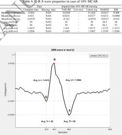
7.1. QRS Waves
The ventricular depolarization of the heart can be repre-sented by three nodes on the heart electrical wave displayed within ECG signal. These are the Q, R and S nodes, known as the QRS complex. The amplitude of QRS represents the polarization and depolarization of the ventricular. The QRS du-ration is the required time for the signal to pass through the ventricular myocardium [31]. The normality of QRS complex is measured by its duration (time interval). A normal duration of the QRS complex is between 0.08 and 0.10 seconds. An in-termediate QRS complex has an interval between 0.10 and 0.12 seconds. While an abnormal QRS time interval is more than 0.12 seconds. Important QRS properties include rise level (Lr), fall level (L f), rise duration (T r), and fall duration (T f). These factors represent the quality of a QRS wave in terms of specify-ing the ventricular depolarization. The rise and fall levels rep-resent length of edges of R peak on the right and left hand side respectively, the rise and fall durations are the required time to move from the Q peak to R peak and from R peak to S peak respectively [32].
Lr=Amplitude R peak - Amplitude Q peak Lf=Amplitude S peak - Amplitude R peak Tr=Time point R peak - Time point Q peak Tf=Time point R peak - Time point Q peak
Mean Error = mean (noisy-ECG (QRS locations) - ((filtered (QRS locations))
7.2. QRS waves and missing values
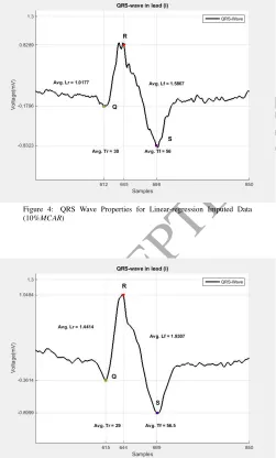
[image:8.595.296.546.343.619.2]The performance of the VAR-IM method is evaluated by comparing the effectiveness of missing data imputation on QRS wave properties, in both cases of missing data (10% and 20% MCAR) and complete data. Furthermore, the efficiency of miss-ing data imputation is considered in the filtermiss-ing processmiss-ing. Figure 2 shows the QRS complex rise level, fall level, rise time and fall time in the case of complete data. In comparison, Fig-ures 3-5 show various results with respect to the case of 10% MCAR. The four proposed techniques with VAR-IM methods were applied to solve the missing data problem here. Clearly, most approaches generated obviously different results: for ex-ample, the list wise deletion could not achieve any improvement in all features; it gave results similar to the case of missing data. on the other hand, all the other methods gave acceptable results, for some features such asLr,L f,T randT f, but the VAR-IM methods still has the highest priority to be the best methods to recover the missing values, which is similar to the real data especially the QRS peaks locations. Table.4 summarizes the re-sults of the effectiveness of missing data imputation of the four methods for the QRS wave properties.
Table 4: Q-R-S wave properties in case of 10% MCAR.
Data Imputed data 10% MCAR missing
Complete data Missing -data VAR-IM List-wise Linear-reg MARSS EM
MeanError Qwave -0.004 NAN -0.0109 - 0.1420 -0.0417 -0.006
MeanError Rwave 0.021 NAN 0.0243 - 0.0277 0.0212 -0.0068
MeanError Swave -0.0155 NAN -0.342 - -0.0576 -0.0147 -0.018
avg riseTime 29 NAN 28 - 30 28.5 28
avg fallTime 56 NAN 59 - 56 56.5 57
avg riseLevel 1.4419 NAN 1.424 - 1.0171 1.4332 1.4312
avg fallLevel 1.9204 NAN 1.9165 - 1.5867 1.9199 1.9296
A
CCE
P
T
E
D
M
A
N
U
S
[image:9.595.294.545.74.272.2]CRIP
T
Figure 3: QRS Wave Properties VAR-IM Imputed Data (10%MCAR)
Figure 4: QRS Wave Properties for Linear-regression Imputed Data (10%MCAR)
Figure 5: QRS Wave Properties for EM Imputed Data (10%MCAR)
Figure 6: QRS Wave Properties for MARSS Imputed data (10%MCAR)
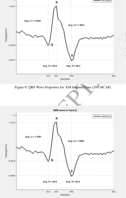
When the percentage of the missing data increases from 10% to 20%, the proposed VAR-IM method gives the best re-sults among the five methods. Table 5 summarizes the rere-sults generated from the recovered data using the five methods, as well as a comparison with that generated from the complete data. As can be noted in both cases of missing data (MCAR 10% and 20%) the MARSS package and EM algorithm have similar results. The reason may be that the MARSS depends mainly on EM algorithm in estimating an MARSS model.
Table 5: Q-R-S wave properties in case of 20% MCAR.
Data Imputed data 20% MCAR missing
Complete data Missing -data VAR-IM List-wise Linear-reg MARSS EM
MeanError Qwave -0.004 NAN -0.0067 - 0.0131 0.0016 0.0014
MeanError Rwave 0.021 NAN 0.0191 - 0.0630 0.022 0.0163
MeanError Swave -0.0155 NAN -0.018 - -0.0802 -0.0096 -0.0191
avg riseTime 29 NAN 29 - 27 28.5 28.5
avg fallTime 56 NAN 56.5 - 429.5 55.5 56.5
avg riseLevel 1.4419 NAN 1.4414 - 0.9402 1.4391 1.4445
[image:9.595.27.274.75.259.2]avg fallLevel 1.9204 NAN 1.9307 - 1.4009 1.9243 1.9341
Figure 7: QRS Wave Properties VAR-IM Imputed Data (20%MCAR)
[image:9.595.26.277.311.727.2]A
CCE
P
T
E
D
M
A
N
U
S
[image:10.595.27.277.75.259.2]CRIP
T
[image:10.595.26.276.316.501.2]Figure 8: QRS Wave Properties for Linear-regression Imputed Data (20%MCAR)
Figure 9: QRS Wave Properties for -EM Imputed Data (20%MCAR)
Figure 10: QRS Wave Properties -MARSS Imputed Data (20%MCAR)
8. Conclusion
It is extremely important to effectively handle multivari-ate data anomalies that contain missing values. This is espe-cially true for medical data, which could involve great num-ber of critical health diagnostic variables. The proposed VAR-IM method provides improvements to speed and accuracy for imputing missing values of multivariate time series datasets. It outperforms the commonly used methods such as list wise deletion, linear regression imputation, MARSS and EM algo-rithms. From the results of the case study, the VAR-IM method provides an effective alternative for the imputation of missing values in multivariate time series. While the other proposed traditional and modern methods become less effective with the increase of the proportion of missing data, VAR-IM shows less deterioration in performance with increasing percentages of miss-ing entries. In addition, the VAR-IM method is more robust than the other proposed techniques when applied to the data types discussed in the case study, and performed better on static and noisy data. There are some limitations of the proposed method. Firstly, this study only considered the scenario in which data was missing completely at random (MCAR), that is, the cause of the missing data was independent of both the observed and missing values. A less stringent assumption of missing data mechanism missing at random (MAR) may be more realistic in practice. MAR refers to the case in which missingness is related to the observed values, but not to the missing values themselves. Secondly, the validity of VAR-IM approach requires that the time series should be stationary. Finally, the percentage of miss-ing data has significant impact on most missmiss-ing data analysis methods, VAR-IM does not have the priority to be used if the percentage of missing data is quite low (say less 10%). Despite these limitations, VAR-IM provides an important alternative to existing methods for handling missing data in multivariate time series. Further extension of the method to include other types of methods will be considered in other future work.
References
[1] J. W. Graham, Missing data: Analysis and design, Springer Science & Business Media, 2012.
[2] J. Schafer, Analysis of incomplete multivariate data, New York: Chapman Hall, 1997.
[3] B. Efron, Missing data, imputation, and the bootstrap, Journal of the American Statistical Association 89 (426) (1994) 463–475.
[4] M. A. Tanner, W. H. Wong, The calculation of posterior distributions by data augmentation, Journal of the American statistical Association 82 (398) (1987) 528–540.
[5] D. Rubin, Multiple imputation for nonresponse in surveys, New York, USA: John Willey & Sons, 1987.
[6] C. K. Enders, D. L. Bandalos, The relative performance of full informa-tion maximum likelihood estimainforma-tion for missing data in structural equa-tion models, Structural Equaequa-tion Modeling 8 (3) (2001) 430–457. [7] J. W. Graham, Missing data analysis: Making it work in the real world,
Annual review of psychology 60 (2009) 549–576.
[8] S. Liu, P. C. Molenaar, ivar: A program for imputing missing data in multivariate time series using vector autoregressive models, Behavior re-search methods 46 (4) (2014) 1138–1148.
[9] L. Ljung, Prediction error estimation methods, Circuits, Systems and Sig-nal Processing 21 (1) (2002) 11–21.
[image:10.595.26.277.335.730.2]A
CCE
P
T
E
D
M
A
N
U
S
CRIP
T
[11] E. E. Holmes, E. J. Ward, K. Wills, Marss: Multivariate autoregressive state-space models for analyzing time-series data, The R Journal 4 (1) (2012) 11–19.
[12] E. Holmes, E. Ward, M. Scheuerell, Analysis of multivariate time-series using the marss package, User guide: http://cran. r-project. org/web/packages/MARSS/vignettes/UserGuide. pdf.
[13] A. P. Dempster, N. M. Laird, D. B. Rubin, Maximum likelihood from incomplete data via the em algorithm, Journal of the Royal Statistical Society. Series B (Methodological) (1977) 1–38.
[14] R. H. Shumway, D. S. Stoffer, An approach to time series smoothing and forecasting using the em algorithm, Journal of time series analysis 3 (4) (1982) 253–264.
[15] J. C. Ag¨uero, W. Tang, J. I. Yuz, R. Delgado, G. C. Goodwin, Dual time–frequency domain system identification, Automatica 48 (12) (2012) 3031–3041.
[16] T. Schneider, Analysis of incomplete climate data: Estimation of mean values and covariance matrices and imputation of missing values, Journal of Climate 14 (5) (2001) 853–871.
[17] R. Gopaluni, A particle filter approach to identification of nonlinear pro-cesses under missing observations, The Canadian Journal of Chemical Engineering 86 (6) (2008) 1081–1092.
[18] R. H. Shumway, D. S. Stoffer, Time series analysis and its applications, Studies In Informatics And Control 9 (4) (2000) 375–376.
[19] G. C. Reinsel, Elements of multivariate time series analysis, Springer Sci-ence & Business Media, 2003.
[20] E. Zivot, J. Wang, Vector autoregressive models for multivariate time se-ries, Modeling Financial Time Series with S-PlusR(2006) 385–429. [21] W. J. Tsay, Maximum likelihood estimation of stationary
multivari-ate arfima processes, Journal of Statistical Computation and Simulation 80 (7) (2010) 729–745.
[22] W. L. Wang, Multivariate t linear mixed models for irregularly observed multiple repeated measures with missing outcomes, Biometrical Journal 55 (4) (2013) 554–571.
[23] H. L¨utkepohl, New introduction to multiple time series analysis, Springer Science & Business Media, 2005.
[24] H. Akaike, A new look at the statistical model identification, IEEE trans-actions on automatic control 19 (6) (1974) 716–723.
[25] G. Schwarz, Estimating the dimension of a model the annals of statistics 6 (2), 461–464, URL: http://dx. doi. org/10.1214/aos/1176344136. [26] E. J. Hannan, B. G. Quinn, The determination of the order of an
autore-gression, Journal of the Royal Statistical Society. Series B (Methodologi-cal) (1979) 190–195.
[27] H. Akaike, Fitting autoregressive models for prediction, Annals of the institute of Statistical Mathematics 21 (1) (1969) 243–247.
[28] S. Johansen, Statistical analysis of cointegration vectors, Journal of eco-nomic dynamics and control 12 (2-3) (1988) 231–254.
[29] R. Bousseljot, D. Kreiseler, A. Schnabel, Nutzung der ekg-signaldatenbank cardiodat der ptb ¨uber das internet, Biomedizinische Technik/Biomedical Engineering 40 (s1) (1995) 317–318.
[30] A. L. Goldberger, L. A. Amaral, L. Glass, J. M. Hausdorff, P. C. Ivanov, R. G. Mark, J. E. Mietus, G. B. Moody, C.-K. Peng, H. E. Stanley, Physiobank, physiotoolkit, and physionet components of a new research resource for complex physiologic signals, Circulation 101 (23) (2000) e215–e220.
[31] N. Burns, Cardiovascular physiology, Retrieved from School of Medicine, Trinity College, Dublin. http://www. medicine. tcd. ie/physiology/assets/docs12 13/lecturenotes/NBurns% 20CVS% 20lec-ture, 2013.
[32] J. Pan, W. J. Tompkins, A real-time qrs detection algorithm, Biomedical Engineering, IEEE Transactions on (3) (1985) 230–236.
A
CCE
P
T
E
D
M
A
N
U
S
CRIP
T
Faraj Bashiris a Ph.D. candi-date at the university of Sheffield, in Automatic Control and Systems Engineering Department, United Kingdom. He re-ceived his B.Sc. and M.Sc. degrees from the University of Tripoli, Faculty of Engineering, Automatic Control and Sys-tems Engineering Department, in 2003 and 2008, respectively. His research interests concern application of missing data anal-ysis, generalised linear models, clustering, pattern recognition, regression, Gaussian processes, system identification; polyno-mial models, VAR modelling, model selection; kernel density estimation and EM algorithm.