White Rose Research Online URL for this paper:
http://eprints.whiterose.ac.uk/133860/
Version: Published Version
Article:
Haslegrave, J. and Jordan, J. (2018) Non-convergence of proportions of types in a
preferential attachment graph with three co-existing types. Electronic Communications in
Probability, 23. 54. ISSN 1083-589X
https://doi.org/10.1214/18-ECP157
© 2018 Institute of Mathematical Statistics. This is an Open Access article distributed
under the terms of the Creative Commons Attribution Licence
(http://creativecommons.org/licenses/by/4.0), which permits unrestricted use, distribution,
and reproduction in any medium, provided the original work is properly cited.
[email protected]
https://eprints.whiterose.ac.uk/
Reuse
This article is distributed under the terms of the Creative Commons Attribution (CC BY) licence. This licence
allows you to distribute, remix, tweak, and build upon the work, even commercially, as long as you credit the
authors for the original work. More information and the full terms of the licence here:
https://creativecommons.org/licenses/
Takedown
If you consider content in White Rose Research Online to be in breach of UK law, please notify us by
ISSN:1083-589X in PROBABILITY
Non-convergence of proportions of types in a preferential
attachment graph with three co-existing types
John Haslegrave
*Jonathan Jordan
†Dedicated to the memory of Chris Cannings
Abstract
We consider the preferential attachment model with multiple vertex types introduced by Antunovi´c, Mossel and Rácz. We give an example with three types, based on the game of rock-paper-scissors, where the proportions of vertices of the different types almost surely do not converge to a limit, giving a counterexample to a conjecture of Antunovi´c, Mossel and Rácz. We also consider another family of examples where we show that the conjecture does hold.
Keywords: preferential attachment; stochastic approximation; social networks; competing types.
AMS MSC 2010:Primary 05C82, Secondary 05C80; 60C05; 90B15. Submitted to ECP on May 29, 2018, final version accepted on July 25, 2018. SupersedesarXiv:1805.10071.
1 Introduction
We consider a model for randomly growing networks of agents having different types, which are not innate but are chosen based on what they see when they join the network. These types might represent social groups, opinions, or survival strategies of organisms. This model was introduced by Antunovi´c, Mossel and Rácz [1], who define a family of preferential attachment random graphs where each new vertex receives one of a fixed number of types according to a probability distribution which depends on the types of its neighbours. Using stochastic approximation methods, they fully deal with the case where there are two types of vertices, and show that the proportions of the vertices which are of each type almost surely converge to a (possibly random) limit which is a stable fixed point of a certain one-dimensional differential equation.
The case where there are more than two types is discussed in Section 3 of [1]. They conjecture (Conjecture 3.2) that the behaviour is always similar to the two-type model in that there is almost sure convergence to a limit which is a stationary point of what is now a multi-dimensional vector field. They confirm this for the case they call the linear model, where the probability each type is chosen is proportional to the number of neighbours of that type the new vertex has. However, the difficulties of a general analysis of the class of vector fields associated to models of this type make it hard for more general results to be proved.
*University of Warwick. E-mail:[email protected]
In this note, we give a model with three types which is a counterexample to Conjecture 3.2 of [1]. The type assignment mechanism in this model is inspired by the well-known game of “rock-paper-scissors”, and we show that in this model the associated vector field does not have attractive stationary points and that the proportions of the types do not converge to a limit, but approach a limit cycle of the associated vector field, so that each type in turn will have the largest proportion of the edges.
We also give a family of examples where we can show that Conjecture 3.2 of [1] does hold. This is where the new vertex chooses uniformly at random from those types represented among vertices which it connects to. In this case, we will show that there is a single stable stationary point of the vector field, which corresponds to the proportions of each type being equal, and that almost surely the proportions of the types will converge to this point asn→ ∞.
2 The Antunovi´
c-Mossel-Rácz framework
The framework introduced by Antunovi´c, Mossel and Rácz in [1] considers a standard preferential attachment graph where the new vertex connects tomexisting vertices as originally suggested by Barabási and Albert in [2], with the different vertices chosen independently as in the “independent model” of [4]. That is, we consider a random sequence of graphsG0, G1, . . .starting from some non-empty fixed graphG0. For each
t >0we choosemrandom vertices fromGt−1independently and with replacement, with
probabilities proportional to their degrees. We then add a new vertex connected bym
edges to the chosen vertices (allowing multiple edges if a vertex is chosen more than once) to formGt.
Each vertex is one ofN types{1, . . . , N}, often referred to in [1] as colours; once it has been assigned, the type of a vertex is fixed for all time. When a new vertex joins the graph, it takes a type based on the types of its neighbours in the following general way, where the notation follows section 3 of [1]. The types of themneighbours induce a vectoru ∈NN0 whose elements sum tom and whoseith element is the number of
neighbours of type i. For each possibleu, we will have a probability distribution on {1, . . . , N}, which we will describe by a vectorpu∈∆
N−1, whoseith element gives the
probability that the new vertex is of typeigiven thatuis the vector giving the numbers of its neighbours of each type. Here∆N−1denotes the(N−1)-dimensional simplex.
The special case wherepu=u/mis referred to in [1] as the linear model. For other
cases, they show (Lemma 3.4) that the sequence of vectorsxn giving the normalised total degrees of the vertices of each type is a stochastic approximation process driven by a vector fieldPwhich depends on thepu, that is we have
xn+1−xn=
1
n P(xn) +ξn+1+Rn
, (2.1)
where the ξi satisfy the martingale difference conditionE(ξn+1|Fn) = 0, withFn =
σ(x0,x1, . . . ,xn), and the Ri are remainder terms satisfying P∞i=1Ri/n < ∞ almost surely. As a result, understanding the vector field P is an important step towards understanding the behaviour of the stochastic process and applying the general results on stochastic approximation processes found in, for example, Benaïm [3] and Pemantle [9].
3 Rock-paper-scissors model
We introduce a model in the framework of [1] where the type assignment mechanism is based on the game of rock-paper-scissors. Cyclic dominance systems of this basic form have been shown to naturally occur in a variety of organisms and ecosystems, ranging from colour morphisms of the side-blotched lizard [10] to strains ofEscherichia coli [8]. Such patterns of dominance can explain biodiversity. Whereas simpler transitive relations necessarily have a single fittest phenotype which, in the absence of other factors, should eventually dominate, cyclic dominance allows for situations where no phenotype has an evolutionary advantage over all others and thus multiple phenotypes may persist.
Itoh [7] investigated a simple Moran process based on the rock-paper-scissors game. A population of fixed size consists of rock-type, scissors-type and paper-type individuals. At each time step two individuals meet and play rock-paper-scissors; the loser is removed and replaced with a clone of the winner. The population is assumed to be well-mixed, so meetings occur uniformly at random; in such a system one type must eventually take over the whole population. Similar processes have also been studied in a more structured environment, such as sessile individuals interacting on the2-dimensional lattice (see e.g. [11]). Here the limited range of interactions allows co-existence of types [8]. While a lattice model may closely approximate the interactions between bacteria growingin vitro, neither a lattice nor a well-mixed model is a good representation of the heterogeneous social interaction networks that arise among more complex organisms; here a model incorporating preferential attachment is more realistic.
Our model hasN= 3types andm= 2, the types1,2and3corresponding to “rock”, “paper” and “scissors” respectively. If the two sampled vertices are of the same type, the new vertex takes that type, whereas if they are of different types they play a game of rock-paper-scissors, playing their type, and the new vertex takes the type of the winner. In the notation above, we have
p(1,1,0)= (0,1,0), p(0,1,1)= (0,0,1), p(1,0,1)= (1,0,0),
p(2,0,0)= (1,0,0), p(0,2,0)= (0,1,0), p(0,0,2)= (0,0,1),
and the vector field P, defined by (3.1) of [1], on the triangle ∆2 is given by the
components
P1(x, y, z) =
x 2(z−y) P2(x, y, z) = y
2(x−z) P3(x, y, z) =
z
2(y−x).
3.1 Limiting behaviour of the model
LetXn,YnandZndenote the total degrees of vertices of types1,2and3respectively, normalised to sum to1. By Lemma 3.4 of [1],(Xn, Yn, Zn)follows a stochastic approxi-mation process (2.1) on the triangle∆2driven by the vector fieldP with the noise terms
ξibounded.
Lemma 3.1.The productxyzis constant on trajectories ofP.
Proof. We have
d
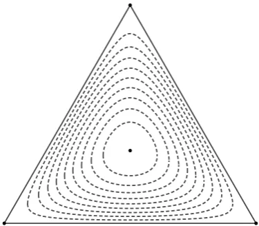
Figure 1: Trajectories on which27xyzis constant (ranging from0.1to0.9).
The vector field has four stationary points: the corners of the simplex, which are saddle points, and(1/3,1/3,1/3), which has eigenvalues±√i
27, making it an elliptic fixed
point. Together with Lemma 3.1 we can see that trajectories ofP circle the centre of the simplex on loops of constantxyz; some of these are shown in Figure 1.
LetMn =XnYnZn. Our main result is the following.
Theorem 3.2.The process(Mn)n∈Nalmost surely converges to a limitM ∈(0,1/27),
and the distribution ofM has full support on (0,1/27). Furthermore, almost surely
(Xn, Yn, Zn)fails to converge; rather its limit set is the set{(x, y, z)∈∆2:xyz=M}.
Remark 3.3.The failure to converge means that this model provides a counterexample to Conjecture 3.2 of [1].
Theorem 3.2 follows from the following three propositions, together with standard results on stochastic approximation processes.
Proposition 3.4.The process(Mn)n∈Nalmost surely converges to a limitM ∈[0,1/27],
and the distribution ofM has full support on(0,1/27).
Proposition 3.5.Almost surelyM = limn→∞Mn<1/27.
Proposition 3.6.Almost surelyM = limn→∞Mn>0.
Proof of Proposition 3.4. Letγn= 4n+ 2e0, that is the total degree inGn; heree0is the
number of edges in the initial graphG0. Then, if the two sampled vertices are both
“rock”, which has probabilityX2
n, we have that
Mn+1γ3n+1= (Xnγn+ 4)YnZnγn2 =Mnγn3+ 4YnZnγ2n,
while if one sampled vertex is “rock” and the other is “paper”, which has probability
2XnYn, we have that
Mn+1γn3+1= (Xnγn+ 1)(Ynγn+ 3)Znγn=Mnγn3+ 3XnZnγn2+YnZnγn2+ 3Znγn,
with analogous expressions for the other possibilities. Hence
E(Mn+1| Fn) =γn−+13 (Mnγ3n+ (4 + 6 + 2)Mnγn2+ (6 + 6 + 6)Mnγn)
=Mn(γn+ 4)−3(γn3+ 12γn2+ 18γn)
=Mn
1− 30
γ2
n+1
+ 56 γ3
n+1
showing that(Mn)n∈N is a supermartingale. It takes values in[0,1/27].
If we let Rn+1 = Mn
30
γ2
n+1−
56
γ3
n+1
and M˜n = Mn +Pnk=1Rk then ( ˜M)n∈N is a
martingale. The differenceM˜n−Mn is bounded, soM˜n→M˜ almost surely, whereM˜ is a random limit.
There exist positive constantsc1, c2such that−γc1n ≤Mn+1−Mn ≤γc2n. Hence there existscsuch thatVar( ˜Mn+1−M˜n | Fn)≤γc2
n and thusVar( ˜M | Fn)→0asn→ ∞.
Given an interval (r, r+ǫ) ∈ (0,1/27), for n large enough there will be positive probability ofMn ∈(r+ǫ/3, r+ 2ǫ/3). ThatVar( ˜M | Fn)→0and thatP∞k=n+1Rk→0 asn→ ∞ ensures that ifnis large enough there is then positive probability ofM ∈
(r, r+ǫ).
In order to prove Proposition 3.5, we will need better control on the variation ofMn+1
ifMnis close to1/27.
Lemma 3.7.If Mn > 271 − γcn then
Mn+1−E(Mn+1 | Fn)
< C
γn3/2
for someC which depends only oncand for sufficiently largen.
Proof. Note that if |Xn− 13| ≥ c
′
√γ
n then Mn ≤ 1 27 −
c′2
4γn +
c′3
4γ3/2
n
. Consequently, for a
suitable choice ofc′ and sufficiently largenwe have|X
n−13|,|Yn−31|,|Zn−13|<
c′
√γ n.
In turn this means that
1 Xn
< 3 1− 3c′
√γ n
= 3 +√9c′ γn +
27c′2
γn−3c′√γn
<3 + √c′′ γn
for somec′′ andnsufficiently large. Similarly we have 1
Xn >3−
c′′
√γ
n, and the same
bounds apply toYn, Zn.
Writeµn+1forE(Mn+1γn3+1| Fn); by (3.1), sinceγn+1=γn+ 4, we have
µn+1=Mnγn3+1−30Mnγn+1+ 56Mn
=Mnγn3+ 12Mnγn2+ 18Mnγn.
With probabilityX2
n we haveMn+1γ3n+1=Mnγn3+ 4YnZnγn2, giving
|Mn+1γ3n+1−µn+1| ≤
4 Xn −
12 Mnγ
2
n+ 18Mnγn
<4c′′ 27γ
3/2
n +
2
3γn< Cγ
3/2
n
for some C and sufficiently large n. With probability 2XnYn we have Mn+1γn3+1 =
Mnγn3+ 3XnZnγ2n+YnZnγn2+ 3Znγn, giving
|Mn+1γn3+1−µn+1| ≤
3 Yn −
9 + 1 Xn −
3 Mnγ
2
n+|3Zn−18Mn|γn
< 4c′′ 27γ
3/2
n + 3γn+
2
3γn< Cγ
3/2
n ,
and similar bounds apply in other cases. Thus we have
Mn+1−E(Mn+1 | Fn)
<
Cγn3/2
γ3
n+1
< C γ3n/2
We are now ready to show that almost surelyMndoes not tend to1/27.
Proof of Proposition 3.5. Suppose for the sake of contradiction that P M = 271
> 0. Then forn0sufficiently large there will be an eventA ∈ Fn0 such thatP M =
1 27 | A
≥
1−ε. Fixc1> c2>0to be chosen later, and letBbe the event that for somen∈[n0,2n0]
we haveMn ∈ 271 −cn1,271 −cn2. We claim that, for suitablec1, c2which do not depend
on n0, we have P(B | Fn0)is bounded away from 0 for n0 sufficiently large. To see
this, stop the process ifMn < 271 −nc20 or ifn= 2n0; writeτ for the stopping time. By
choice ofτ, it follows from (3.1) thatMn(τ+1) +
Pmin(n,τ) k=n0
1
γ2
k
is a supermartingale, since
30Mn(τ)≥30 271 −nc1
0
>1.
IfBfails, we must haveτ= 2n0andM2n0>
1 27−
c2
2n0, i.e.
M2(τn)0+
2n0−1
X
k=n0 1 γ2 k > 1 27+ a n0
for some constant a, which is positive for suitable choice of c2. Applying Azuma–
Hoeffding, using Lemma 3.7, this occurs with probability bounded away from1. SupposeBoccurs, withτ =n1. LetCbe the event thatMn∈ 271 −2nc1
1,
1 27−
c2
2n1
for everyn≥n1. We claim thatP(C | Fn1)is bounded away from0. The proof is similar: fix n2> n1and stop the process if it leaves the interval or ifn=n2, with stopping timeτ′.
IfCfails to hold beforen2then we have, evaluated atn=n2, either
M(τ′)
n > Mn1− c2
2n1
(3.2)
or
Mn(τ′)− n−1
X
k=n1 2 γ2
k
< Mn1− c1
n1
. (3.3)
Since the left-hand sides of (3.2) and (3.3) are respectively a supermartingale and submartingale, with variations bounded by Lemma 3.7, again by Azuma–Hoeffding this has probability bounded away from1, where the bound is independent ofn1andn2.
Finally, we show that almost surely the limitM is positive.
Proof of Proposition 3.6. First we claim that almost surelyMn = Ω(γn−1). Indeed, in a standard preferential attachment process the degree of a fixed vertexvi satisfies
dn(vi) = (1+o(1))ξi√γn, whereξiis a random variable which is almost surely positive: see Theorem 8.2, Lemma 8.17 and Exercise 8.13 of [6]. Thus the contribution of the starting vertices alone ensures thatmin(Xn, Yn, Zn) = Ω(γn−1/2)and soXnYnZn= Ω(γn−1).
As in the proof of Lemma 3.7, with probabilityX2
n we have
Mn+1γn3+1−µn+1= (4YnZn−12Mn)γn2−18Mnγn;
note that
X2
n (4YnZn−12Mn)γn2−18Mnγn
2
=O(M2
nγn4).
With probability2XnYnwe have
Mn+1γn3+1−µn+1= (3XnZn+YnZn−12Mn)γn2+ (3Zn−18Mn)γn,
and
2XnYn (3XnZn+YnZn−12Mn)γn2+ (3Zn−18Mn)γn
2
=O(Mnγn4).
Similar expressions hold for the other possibilities, giving Var(Mn+1γn3+1 | Fn) =
0.0 0.2 0.4 0.6 0.8 1.0 27M10000
0.0 0.5 1.0 1.5 2.0 2.5 3.0 3.5 4.0
Relative frequency
G0= K3
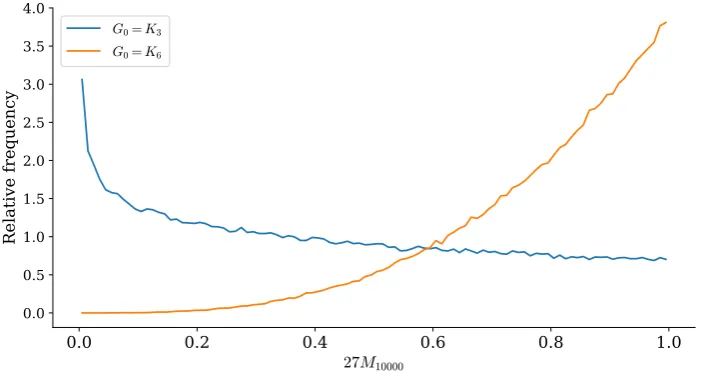
[image:8.595.122.474.102.290.2]G0= K6
Figure 2: Distributions of the value of27M10000from two different starting graphs.
SupposeMn′ <2Mn for alln′ ≥n. Then we haveVar(Mn′+1 | Fn′) =O(Mnγn−2)for eachn′ ≥ n, giving Var(M | Fn) = O(Mnγ−1
n ) =O(Mn2). Thus there is a probability bounded away from0asn→ ∞thatM is in the interval(Mn/2,3Mn/2)conditional on Fn, but ifM = 0has positive probability then for anyε >0andnsufficiently large there is an eventA ∈ FnwithP(M = 0| A)>1−ε, giving a contradiction.
We can now complete the proof of our main result.
Proof of Theorem 3.2. Propositions 3.4, 3.5 and 3.6 show that the limit setL(X, Y, Z)is, almost surely, contained within{(x, y, z)∈∆2 :xyz =M}, whereM ∈(0,1/27)is the
random variable defined in Proposition 3.4. By Theorem 5.7 of Benaïm [3],L(X, Y, Z)is almost surely a chain transitive set for the flow; here a chain transitive set for the flow is an invariant setM for the flow such that for every pair of pointsaandbinM and for anyδ >0andT >0there is a(δ, T)-pseudo-orbit fromatob, meaning a finite sequence of partial trajectories, with the first starting ataand the last starting atb, the duration of each trajectory at leastT, and the finishing point of one trajectory and the starting point of the next at mostδapart. ForM ∈(0,1/27)the only invariant set for the flow, and hence the only chain transitive set, which is a subset of{(x, y, z)∈∆2:xyz=M}is
the whole set.
The distribution ofM will naturally depend critically on the starting graphG0. Figure
2 shows approximate distributions for two particular choices ofG0, being the complete
graphs on3and6 vertices respectively, each with equal numbers of rock, paper and scissors vertices. These distributions were taken from simulations to time10000.
3.2 Rate of circling
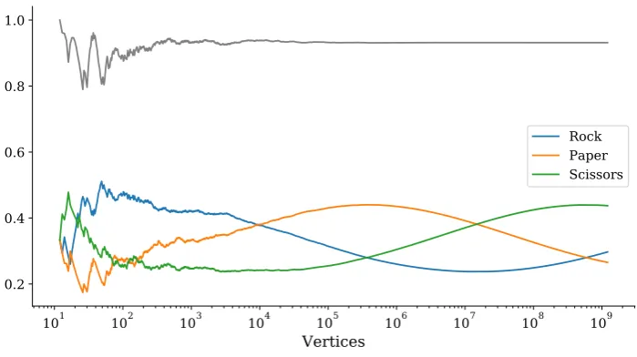
In this section we show that circling around the limiting cycle occurs on a logarithmic scale asn→ ∞, at a rate which depends only on the limit parameterM; this is consistent with the behaviour seen in Figure 3.
Theorem 3.8.Forn0sufficiently large depending onM = limn→∞Mn, with high prob-ability the process completes a circuit approximating the trajectoryMn =M at time
101 102 103 104 105 106 107 108 109
Vertices
0.2 0.4 0.6 0.8 1.0
[image:9.595.121.471.102.298.2]Rock Paper Scissors
Figure 3: Evolution ofXn, Yn, Zn from a simulation, together with27Mn(grey curve).
Proof. For (x, y, z) ∈ ∆2, write f(x, y, z)for
x(z−y) 2 ,
y(x−z) 2 ,
z(y−x) 2
. For anyδ > 0, if
min(x, y, z)∈(δ,1/3−2δ)thenf(x, y, z)is bounded away from0, since assuming without loss of generality thatxis the median value we have|x(z−y)|> δ/3, and triviallyf is also bounded above. Similarly we may bound all partial derivatives off(x, y, z)away from0whenmin(x, y, z)∈(δ,1/3−2δ).
Let CM be the curve{(x, y, z) ∈ ∆2 : xyz =M}, and letL
M be its length (in the Euclidean metric). Fixδ >0such thatM ∈(δ,1/27−δ). Letε∈(0, δ2)be arbitrary, and
supposen0is sufficiently large that|Mn−M|< ε2for alln > n0with high probability.
Note that, conditioned on this event, we must havemin(Xn, Yn, Zn)∈(δ,1/3−2δ)for all
n > n0and sof(Xn, Yn, Zn)is bounded away from0.
Writeni+1=⌊(1 +ε)ni⌋fori≥0and consider the process(Xn, Yn, Zn)forn∈[n0, n1].
Think of this as an urn process, where balls represent edge-ends; for each vertex we draw two balls from the urn, replace them and add four new balls depending on the draw. For the moment, only reveal the information of whether each ball drawn was in the urn at timen0or not; call a vertex “typical” if both balls drawn for that vertex were in at timen0.
The number of atypical vertices is dominated by a binomial(⌊εn0⌋,2ε)random variable,
so we have at least(ε−3ε2)n
0 typical vertices with high probability. Now the type of
new balls added for each typical vertex are independent and identically distributed, contributing on average4εn0Xn0 1 +
Zn0−Yn0
2
rock,4εn0Yn0 1 +
Xn0−Zn0
2
paper and
4εn0Zn0 1 +
Yn0−Xn0
2
scissors to the urn, so the variance of numbers of each type contributed by typical vertices isO(εn) =o(ε2n2). Consequently with high probability at
timen1the number of balls of type rock is at least4n0Xn0+ 4εnXn0 1 +
Zn0−Yn0
2
−4ε2n
and at most4n0Xn0+ 4εnXn0 1 +
Zn0−Yn0
2
+ 4ε2n
0, and similarly for paper and scissors.
It follows that the distance from (Xn0, Yn0, Zn0) to (Xn1, Yn1, Zn1) is within 12ε
2
of 2(1+εε)f(Xn0, Yn0, Zn0), and similarly for eachi the distance from (Xni, Yni, Zni)to
(Xni+1, Yni+1, Zni+1) is within12ε
2 of ε
2(1+ε)f(Xni, Yni, Zni), both with high probability.
Note that, since partial derivatives off are bounded away from 0, f(Xni, Yni, Zni)− 1
is withinO(ε2) of f(x
i, yi, zi)−1, where we define(xi, yi, zi) to be the closest point to
(Xni, Yni, Zni)onCM.
[(1 +ε)b/εn0,(1 +ε)B/εn0], i.e. in[ebn0,eBn0].
Lettingε→0gives the required result withA= exp 2LMRt∈CMf(t)−1dt.
3.3 Affine preferential attachment
A natural extension of the model of [1], considered briefly in that paper, is where we have affine preferential attachment so that a vertexvis chosen for attachment with probability proportional tod(v) +αfor someα >−2. Affine preferential attachment was introduced by Dorogovtsev, Mendes and Samukhin in [5]. It turns out that the behaviour of the rock-paper-scissors model is similar in this modified setting. LetXn, Yn, Zn be the probabilities of selecting rock, paper and scissors vertices respectively by a single preferential choice at timen, letMn=XnYnZn, and writeγn=Pv(dn(v) +α). Now with probabilityX2
nwe haveγn3+1Mn+1= (γnXn+ 4 +α)γnYnγnZn, with probability2XnYn we haveγ3
n+1Mn+1= (γnXn+ 1)(γnYn+ 3 +α)γnZn, and so on, giving
E(Mn+1| Fn) =γn−+13 (Mnγn3+ (12 + 3α)Mnγn2+ (18 + 6α)Mnγn)
=Mn(γn+ 4 +α)−3(γn3+ (12 + 3α)γn2+ (18 + 6α)γn)
=Mn
1−(30 + 18α+ 3α
2)γ
n
γ3
n+1
−(4 +α)
3
γ3
n+1
.
As in the proof of Proposition 3.4, noting that30 + 18α+ 3α2≥3, we have that(M
n)n∈Nis
a supermartingale with the appropriate variance properties, meaning that Propositions 3.4 and 3.5 apply as in the standard model. Forα >0, however, the proof of Proposition 3.6 does not translate to this setting, since the degree of a given vertex grows as
γ1n/(2+α/2).
IfM = 0then{(x, y, z)∈∆2:xyz = 0} is a chain transitive set, but the stationary
points at the corners of the triangle are also chain transitive sets. However, we can prove that the corners are limits with probability zero. Without loss of generality, assume
(Xn, Yn, Zn)→(1,0,0). Then, fornsufficiently largeXn>1/2, meaning that conditional onFnthe probability that vertexn+1is of type2(paper),Y2
n+2XnYn> Yn. Consequently we can boundYn below by the proportion of black balls in a coupled standard Pólya urn process, showing thatP(Yn→0) = 0on the eventXn>1/2fornlarge enough. Hence
P(L(X, Y, Z) = (1,0,0)) = 0. Thus we have the following slight weakening of Theorem 3.2 for this setting.
Theorem 3.9.For affine preferential attachment, the process(Mn)n∈Nalmost surely
converges to a limitM ∈[0,1/27), and the distribution ofM has full support on(0,1/27). Furthermore, almost surely(Xn, Yn, Zn)fails to converge; rather its limit set is the set {(x, y, z)∈∆2:xyz=M}.
4 Pick random visible type
We now consider another natural, simple rule for choosing types; instead of copying the type of a random neighbour, as in the linear model, we choose uniformly at random between types present in the neighbourhood. This method gives common types slightly less advantage than the linear model, and instead of almost sure convergence to a random limit, here we obtain almost sure convergence to a deterministic limit.
Theorem 4.1.Suppose we have N ≥ 2 types and each new vertex chooses m ≥ 3
neighbours, and adopts a type chosen uniformly at random from those present among its neighbours. Then the proportion of each type converges almost surely to1/N.
Remark 4.2.Ifm= 2then this model reduces to the linear model of [1].
to show that lim infn→∞Xn(N) ≥ 1/N almost surely, since by symmetry of the model the same will apply to all other types, implying thatXn(i) →1/N; convergence of the proportions of vertices follows by considering the vertices added once|Xn(i)−1/N|< ε for eachi.
We couple the process with a two-type process as follows. Treat all types other than typeN as indistinguishable, forming a single supertype∗, and letYn be the proportion of edge-ends of typeN at timen. Join each new vertex tomvertices as before. If each of the chosen vertices has the same type, assign that type to the new vertex. Otherwise, ifkvertices are chosen from type∗andm−kfrom typeN with0< k < m, samplek
independent variables from the uniform distribution on{1, . . . , n−1}and letZ(k)be the number of different values seen; now assign typeN to the new vertex with probability
1
Z(k)+1.
By Lemma 4.3 below, for everykandj we have
P(Z(k)≥j)≥P(An+1≥j|Bn+1=k,Fn),
whereAn+1is the number of types other thanNamong neighbours ofvn+1in the original
process, andBn+1is the number of neighbours not of typeN; it follows that
E 1
Z(k) + 1
≤E 1
An+1+ 1
Bn+1=k,Fn
.
ProvidedXn(N)≥Yn, we have
P(vn+1has typeN | Fn) =
m−1
X
k=0
P(Bn+1=k)E
1
An+1+ 1
Bn+1=k,Fn
≤ m−1
X
k=0
m k
(1−Yn)k(Yn)m−kE
1
Z(k) + 1
,
and so it is possible to couple the two processes such thatXn(N)≥Yn. Writing
f(y) =
m−1
X
k=0
m
k
(1−y)kym−k
E 1
Z(k) + 1
−y,
we have
Yn+1−Yn =
f(Yn) +ξn+1
γn+1
,
whereγn is the number of edge-ends at timenandξnis a random variable satisfying
E(ξn | Fn) = 0 and |ξn| < m+ 1. It is straightforward to check that this is a one-dimensional stochastic approximation process satisfying the conditions of Pemantle [9], Section 2.4, and hence Corollary 2.7 of [9] implies thatYnconverges to a zero off.
We claim thatf(y)>0for0< y <1/N. To see this, note thatf(y)is the difference in probability of the new vertex selecting typeN in the linear model (copying the type of a random neighbour) over this model, assuming that the proportion of type-N edge ends isy, and proportions of other types are equal. We condition on the types represented in the neighbourhood; the only cases which contribute are those whereN is represented. Given that typeN andkspecified other types are represented, the expected number of neighbours of typeN is at most that of each other type, so is at mostkm+1. Thus the probability of selecting typeN, given which types are represented, is no greater in the linear model than in this model. This inequality is strict provided0 < k < m−1 (if
N ≥2, the inequality is strict in at least one case with positive probability of occurring, and sof(y)>0.
ThusYn →0orlimYn≥1/N, so it suffices to show thatYn6→0. This follows since if
Yn →0then we haveYn<1/N fornsufficiently large, and sincef(y)≥0ify≤1/N we can couple to a standard Pólya urn.
We conclude by proving the inequality required for the two-type coupling.
Lemma 4.3.Fixn≥1,m≥0andk≥0, and letpbe a probability distribution on[n]. Then the probabilitypn,m,k(p)that a sample ofmindependent variables with distribution pincludes at leastkdifferent elements of[n]is maximised whenp= (1/n, . . . ,1/n), and moreover whenn, m≥k≥2that is the unique maximiser.
Proof. The statement is trivial unlessn, m≥k≥2since ifmin(n, m)< kthenpn,m,k(p)≡
0 and if n, m ≥ k < 2 then pn,m,k(p) ≡ 1. When n, m ≥ k ≥ 2, we prove that if p=p1, . . . , pnis a non-uniform probability distribution then it does not maximisepn,m,k(p) by induction onn, with base casen= 2; in this case we havepn,m,k(p) = 1−pm1 −(1−p1)m
and it is easy to see (e.g. by calculus) that this is uniquely maximised whenp1= 1/2.
Supposen >2but the result holds for smaller values ofn; note that any distribution with full support gives pn,m,k(p) > 0, and so we may assume that pi 6= 1for each i. If additionally pis non-uniform, there exists some i for which pi > 0 and the other probabilities are not all the same; without loss of generality, assumei=n. We condition on the number of timesnappears in the sample, so that
pn,m,k(p) = (1−pn)mpn−1,m,k(q) + m X
j=1
m j
pjn(1−pn)m−jpn−1,m−j,k−1(q),
whereq= p1
1−pn, . . . ,
pn−1
1−pn
is the conditional distribution ifnis not selected. Applying the induction hypothesis toq, equalisingp1, . . . , pn−1will not decrease any term, and will
strictly increase at least one term (the initial term ifn > kor thej= 1term otherwise), sopdoes not maximisepn,m,k(p).
References
[1] T. Antunovi´c, E. Mossel, and M. Rácz,Coexistence in preferential attachment networks, Combinatorics, Probability and Computing25(2016), 797–822. MR-3568948
[2] A.-L. Barabási and R. Albert,Emergence of scaling in random networks, Science286(1999), 509–512. MR-2091634
[3] Michel Benaïm,Dynamics of stochastic approximation algorithms, Séminaire de Probabilités, XXXIII, 1–68, Lecture Notes in Math.1709(1999). MR-1767993
[4] N. Berger, C. Borgs, J. Chayes, and A. Saberi,Asymptotic behaviour and distributional limits of preferential attachment graphs, Annals of Probability42(2014), 1–40. MR-3161480 [5] S. N. Dorogovtsev, J. F. F. Mendes, and A. N. Samukhin,Structure of growing networks with
preferential linking, Physical Review Letters85(2000), 4633–4636.
[6] R. van der Hofstad,Random graphs and complex networks. Vol. 1, Cambridge Series in Statistical and Probabilistic Mathematics43. Cambridge University Press, 2017. MR-3617364 [7] Y. Itoh,On a ruin problem with interaction, Ann. Instit. Statst. Math.25(1973), 635–641.
MR-0346951
[8] B. Kerr, M. A. Riley, M. W. Feldman, and B. J. M. Bohanna,Local dispersal promotes biodiver-sity in a real-life game of rock-paper-scissors, Nature418(2002), 171–174.
[9] R. Pemantle,A survey of random processes with reinforcement, Probability Surveys4(2007), 1–79. MR-2282181
[11] G. Szabó, A. Szolnoki, and R. Izsák,Rock-scissors-paper game on regular small-world net-works, J. Physics A37(2004), 2599–2609. MR-2047229
Acknowledgments.The first author was supported by the European Research Council