Terrestrial laser scanning for building information modelling (BIM) development and application

University of Southern Queensland

Faculty of Engineering and Surveying

Terrestrial Laser scanning for Building

Information Model (BIM) Development and

Application

A dissertation submitted by

Mr Brenton Light

In fulfilment of the requirements of

Bachelor of Spatial Science

i

ABSTRACT

Terrestrial laser scanners (TLS) offer the ability to collect highly accurate high density 3D point clouds. This dissertation looks into errors evident in TLS scans, such as edge effects, ranging errors, noise, and effect of surface reflectivity with the project scanner (which is a Trimble TX5). It then goes on to analyse the magnitude of these errors and ultimately concludes that the TLS is a suitable tool for use in Building Information Modelling (BIM)

ii

University of Southern Queensland Faculty of Health, Engineering and Sciences

ENG4111/ENG4112 Research Project

LIMITATIONS OF USE

The Council of the University of Southern Queensland, its Faculty of Health, Engineering & Sciences, and the staff of the University of Southern Queensland, do not accept any responsibility for the truth, accuracy or completeness of material contained within or associated with this dissertation.

Persons using all or any part of this material do so at their own risk, and not at the risk of the Council of the University of Southern Queensland, its Faculty of Health, Engineering & Sciences or the staff of the University of Southern Queensland.

iii

University of Southern Queensland Faculty of Health, Engineering and Sciences

ENG4111/ENG4112 Research Project

CERTIFICATION OF DISSERTATION

I certify that the ideas, designs and experimental work, results, analyses and conclusions set out in this dissertation are entirely my own effort, except where otherwise indicated and acknowledged.

I further certify that the work is original and has not been previously submitted for assessment in any other course or institution, except where specifically stated.

iv

ACKNOWLEDGEMENTS

This research project was carried out under the principal supervision of Dr Zhenyu Zhang. His assistance in this project has been greatly appreciated.

This project has taken extensive research and implementation. It has taken great effort from not only myself but my wife in picking up the slack at home whilst I spend countless hours working on this project. For this I thank her. I also thank both my daughters for their endless patience throughout this year.

This project would also not have been possible without the generosity of Ultimate Positioning Group who made the TX5 laser scanner available for use, for this I thank them.

TABLE OF CONTENTS

ABSTRACT I

LIMITATIONS OF USE II

CERTIFICATION OF DISSERTATION III

ACKNOWLEDGEMENTS IV

TABLE OF CONTENTS 1

LIST OF FIGURES 4

LIST OF TABLES 5

CHAPTER 1–INTRODUCTION 6

1.1 Introduction ... 6

1.2 The problem ... 7

1.4 Research Objectives ... 7

CHAPTER 2–LITERATURE REVIEW 8 2.1 Introduction ... 8

2.2 Building Information Modelling ... 8

2.1.1 Definition ... 9

2.1.2 BIM for existing buildings ... 9

2.1.3 Industry Foundation Classes ... 10

2.1.4 Level of Development ... 10

2.2 Terrestrial Laser Scanners ... 11

2.2.1 Types of Terrestrial Laser Scanner ... 12

2

2.2.4 Combining BIM with Terrestrial Laser Scanners ... 19

CHAPTER 3–METHODOLOGY 20 3.1 The Laser Scanner ... 20

3.2 Accuracy Testing ... 21

3.2.1 Ranging ... 22

3.2.2 Noise ... 22

3.2.3 Edge effects ... 23

3.2.4 Surface Reflectivity ... 24

3.3 Building Information Modelling Software ... 25

3.4 The Sites ... 26

3.3.1 Site 1 – Modern Office Building ... 26

3.3.2 Site 2 – Industrial Shed ... 26

3.3.3 Site 3 – Homestead ... 27

CHAPTER 4–RESULTS AND ANALYSIS 27 4.1 Accuracy Testing ... 28

4.1.1 Ranging ... 28

4.1.2 Noise ... 32

4.1.3 Edge Effects ... 36

4.1.4 Surface reflectivity ... 39

4.2 The Building Scans ... 42

4.2.1 Site 1: Modern Office Building... 43

4.2.2 Site 2 – Industrial Shed ... 46

4.2.3 Site 3 – Homestead ... 49

4.2.4 Conclusions ... 51

4.3 Building Information Modelling ... 55

4.3.1 Converting and Importing the Cloud ... 55

3

4.3.3 Accuracy of the Model ... 57

CHAPTER 5–CONCLUSION 59

5.1 Further Work ... 60

REFERENCES 61

APPENDIX 1 A

APPENDIX 2 B

APPENDIX 3 C

APPENDIX 4 D

APPENDIX 5 E

APPENDIX 6 F

4

LIST OF FIGURES

Figure 1- Fundamental LOD Definitions - BIMForum.org ... 11

Figure 2- Faro Laser Scanner with rotating mirror highlighted ... 16

Figure 3- Edge Detection ... 17

Figure 4- Trimble TX5 Laser Scanner - http://www.trimble.com/3d-laser-scanning/3d-scanners.aspx ... 20

Figure 5- Colour Test Board ... 24

Figure 6- Manual Survey BIM of Strathneath Homestead ... 27

Figure 7. Angle Testing - Traverse Layout ... 28

Figure 8. Angle Testing - Sphere 2 ... 29

Figure 9. Angle Testing - Sphere 3 ... 30

Figure 10- Noise Testing at a Distance - Noise vs Quality ... 33

Figure 11- Noise Testing up Close ... 35

Figure 12- Edge Effect - Accuracy x2 ... 37

Figure 13- Edge Effect - Accuracy x3 ... 37

Figure 14- Edge Effect - Accuracy x4 ... 38

Figure 15- Edge Effect - Accuracy x6 ... 38

Figure 16- 3D View of Colour Test Board Scan... 40

5

LIST OF TABLES

6

CHAPTER 1 – INTRODUCTION

1.1

Introduction

Building information model (BIM) provides detailed information on building components, geometry, spatial relationships, and other properties in three-dimensional (3D) space. BIM helps understand geometric properties of buildings and provides the base for a number of forms of functional analysis and has many applications in areas such as facility management, maintenance, heritage protection, deformation monitoring, town planning and the support of construction decisions. The key idea behind a BIM is to obtain accurate 3D building data in order to adequately describe the buildings structure.

Terrestrial laser scanners (TLS) offer the ability to collect highly accurate high density 3D point clouds. Applications of TLS in BIM have not yet been extensively tested. Moreover, effective methods and workflows for efficiently extracting building structure information from large TLS data sets have yet to be developed.

7

1.2

The problem

Terrestrial laser scanners have not been a technology that has caught on very quickly in the more conventional side of the surveying industry. With historically high startup costs for field equipment, and the very high demands on computing power required to process the immense data sets. Surveyors have been put off delving into this realm for quite a while.

Building information modelling has been the realm of the architects and engineers since its inception in in the late 1970’s (Epstein 2012). Surveyors have been reluctant to enter into this new field, opting to stay with the more familiar CAD arena and three dimensional cad modelling.

1.4 Research Objectives

8

CHAPTER 2 – LITERATURE REVIEW

2.1 Introduction

This chapter will review the literature for both Building Information Modelling and Terrestrial Laser Scanners in order to obtain an understanding of the two and how they might be used together. It will look at an understanding of these two relatively new technologies and what is being done to use these technologies and streamline the process of collecting and processing data.

2.2 Building Information Modelling

9

2.1.1DEFINITION

In ISO 29481-1:2010 the International Standards Organisation defines a building construction information model as:

Shared digital representation of physical and functional characteristics of any built object (including buildings, bridges,

roads, etc.) which forms a reliable basis for decisions.

This is a very vague and broad reaching definition. One that seems to recur endlessly when researching the topic of BIM.

Essentially when looking at the definition, is it seems that BIM reflects the change from the use of analog tools to digital ones (Epstein 2012). Perhaps the most important thing to take from the inability to find a definitive definition of BIM is that it is many different things to many people. To a surveyor the BIM should be whatever the end client desires, not what the surveyor wants to create.

2.1.2 BIM FOR EXISTING BUILDINGS

10

2.1.3 INDUSTRY FOUNDATION CLASSES

Industry Foundation Classes (IFC) provide software applications in the field of architecture, engineering and construction that are IFC compliant with a platform for the exchange of information (Bazjanac & Crawley 1997). Whilst an important, and widely discussed topic, it is outside of the scope of this project. The only thing we need to consider is, when choosing a software package later in the project, it is important that the package be IFC compliant in order to ensure maximum compatibility with potential clients.

2.1.4 LEVEL OF DEVELOPMENT

11 Figure 1- Fundamental LOD Definitions - BIMForum.org

For the purposes of this research project LOD will not be considered, however it is important that the purpose of this project is to investigate construction building information models at a level that will include simple architecture such as walls, floors, and ceilings. In addition it will look at modelling locations of things like windows and doors. It will not look into modelling accurate models of individual components from TLS point clouds such as light fittings, furniture, or other detailed information.

2.2 Terrestrial Laser Scanners

12

Historically, this was probably correct, with TLS costing in the multiple hundreds of thousands of dollars and the processing power required to handle such large datasets costing similarly prohibitive amounts. This has resulted in TLS being slow to be embraced by the general surveying industry, and as such remained the domain of some of the larger more specialized architectural, engineering and construction companies.

Vast leaps in technology has brought the computer power required to handle the large datasets into the realm available in normal office PC’s. At the same time the cost of TLS is now in similar price brackets to the more conventional survey equipment like RTK GPS’ and Robotic Theodolites. Such that many surveyors are starting to look to this equipment to deliver their end customers with new and exciting products.

2.2.1 TYPES OF TERRESTRIAL LASER SCANNER

Terrestrial laser scanners can be broken up into two broad categories based on the method with which they determine the distance to the point being scanned. These are known as time-of-flight laser scanners and phase-shift laser scanners (Vandezande, Krygiel & Read 2013).

Time of Flight Laser Scanner

13

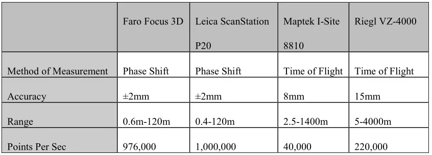
return to the optical sensor. Time of Flight laser scanners have a very long range, with units like the Reigl VZ-4000(Riegl 2013) and Maptek(Maptek 2013) stating on their brochures that they are capable of distances into the multiples of kilometers with precisions of approximately 8-10mm.

Scanning rates for time of flight laser scanners are generally considered slower than those of phase based laser scanners, however the speed of time of flight scanners is rapidly increasing, with the Reigl VZ-4000 capable of up to 220,000 points per second (Riegl 2013).

Phase Shift Laser Scanner

Phase shift laser scanners measure the shift of phase between an emitted laser pulse compared to the light that it receives back to the sensor once it has bounced off the target being measured (Vandezande, Krygiel & Read 2013). When compared to time of flight laser scanners, the distance ranges are considerably shorter. With ranges of 120m for the Leica ScanStation P20 (Leica-Geosystems 2013) out to 330m for the Faro Focus3D X 330 (Faro 2013).

Scan rates for phase shift laser scanners are a lot higher than for those of time of flight scanners, with measurement rates nearing 1 million points per second typical in this class of scanner.

14

As a quick comparison of the different laser scanners and their specifications, see the Table 1 – Comparison of different Laser Scanners below.

Table 1 – Comparison of different Laser Scanners

Faro Focus 3D Leica ScanStation P20

Maptek I-Site 8810

Riegl VZ-4000

Method of Measurement Phase Shift Phase Shift Time of Flight Time of Flight

Accuracy ±2mm ±2mm 8mm 15mm

Range 0.6m-120m 0.4-120m 2.5-1400m 5-4000m

Points Per Sec 976,000 1,000,000 40,000 220,000

2.2.3 ACCURACY OF LASER SCANNERS/POTENTIAL ERRORS

Before using a laser scanner in a BIM situation a surveyor must first fully understand the errors and limitations inherent in a laser scanner. This is because the surveyor must fully understand the data the laser scanner and its software outputs, so that it can be utilized correctly.

15

Studies into the Accuracy of Laser Scanners

There have been many investigations into the accuracy of laser scanners and the way they perform under different conditions.

Boehler, Bordas Vicent, & Marbs (2003) investigated the accuracy of laser scanners extensively. They looked into a number of errors and accuracies inherent in laser scanners. They investigated such potential errors as angular accuracy, range accuracy, resolution, edge effects, and surface reflectivity. Their analysis of the laser scanners available at the time of the study was extensive and well laid out, however these results may potentially no longer be applicable with the advances in scanner technology over the last decade. This will be investigated later on in the practical section of this project.

16

Angular Accuracy

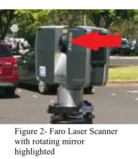
In a terrestrial laser scanner the laser pulse is deflected by a small rotating device (Figure 2- Faro Laser Scanner with rotating mirror highlightedsuch as a mirror or prism and sent to the object being measured, the second angle is usually changed by a mechanical axis or other optical device. These two angles, similar to a conventional total station are used to compute the three dimensional coordinates. Any errors inherent in the laser scanners angular measurement, will obviously be extrapolated perpendicular to the pulse (Boehler, Bordas Vicent & Marbs 2003).

Range Accuracy

As previously stated, terrestrial laser scanners compute their range using either time of flight or phase comparison principles. When scanners don’t have a defined reference point as is often the case when using modern scanners, then it is not possible to measure direct range errors of the instrument. It is only possible to measure range differences between targets (Boehler, Bordas Vicent & Marbs 2003).

Figure 2- Faro Laser Scanner with rotating mirror

17

Resolution

Resolution of a laser scanner is quoted differently by manufacturers and their respective products, it generally a variable setting, up to a maximum value. Maximum resolution of a terrestrial laser scanner is essentially a function of the minimum angular increment possible by the instrument between consecutive points, and the size of the laser spot being produced by the instrument (Boehler, Bordas Vicent & Marbs 2003).

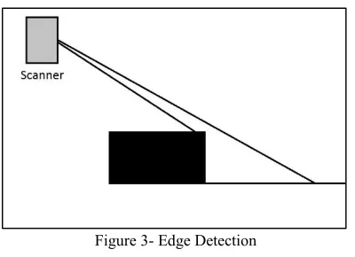
Edge Effects

Edge effects occur when the focused laser spot hits an object edge. Since the laser has a finite size, part of the laser is reflected by the object and part of it reflected by the surface behind the edge, or nothing at all. As depicted in Figure 3- Edge Detection. This can produce incorrect points being calculated as part of a scan. The

range error in these points can vary in magnitude from a fraction of a millimeter to several decimeters (Boehler, Bordas Vicent & Marbs 2003).

18

Effect of Surface Properties

Much like the reflector-less measurement of a total station, laser scanners rely on the laser pulse they emit to be reflected back from the surface they are measuring. The strength of the return of this pulse is dependent on many factors including distance, atmospheric conditions, angle of incidence, and the reflective properties of the object being scanned (Boehler, Bordas Vicent & Marbs 2003).

Environmental Considerations

As mentioned previously, atmospheric conditions play a part in the accuracy of a terrestrial laser scanner. The environmental conditions can also play a part in accuracy of the scanner.

As with any other high accuracy electronic equipment, scanners will only work when used within a specific temperature range (Boehler, Bordas Vicent & Marbs 2003). For example the Faro Focus 3D is stated to work in an ambient temperature range of 5º - 40 ºCelcius (Faro 2013).

19

2.2.4 Combining BIM with Terrestrial Laser Scanners

There already exists research and studies into the automatic extraction of building features from point cloud data sets that have been created by terrestrial laser scanners.

More traditional methods (not utilizing terrestrial laser scanners) for as-built building information modelling mainly involve creating a two dimensional manual reconstruction of the layout from conventional surveying techniques. Then simply elevating this to a certain height to create a three dimensional model (Pu & Vosselman 2006).

Automatic Feature Reconstruction

A number of studies have been carried out regarding automatic extraction of features from laser scanned point clouds. The idea of as-constructed building information models is now a possibility with the rise of cost effective terrestrial laser scanners (Tang et al. 2010).

20

CHAPTER 3 –METHODOLOGY

3.1 The Laser Scanner

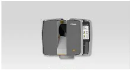
The research component of this project is going to involve investigating the accuracy and suitability of a terrestrial laser scanner for building information modelling. For this project I will be using a Trimble TX5 Laser Scanner (Figure 4) which has been generously supplied by Ultimate Positioning. The TX5 Scanner uses a phase shift measurement technique, has a stated ranging error of ±2mm and can measure point at rates up to 976,000 per second (Trimble 2012). The TX5 does not require an external data collector or laptop and holds its battery within itself. Which makes for a very small, and light unit, weighing only 5.0kg,

21

3.2 Accuracy Testing

For the purposes of this project, we are not interested in testing every accuracy criteria as discussed earlier as some, such as resolution and angular accuracy, are extremely time consuming to test and not really relevant to this project.

The errors we will be considering as a part of this research will be:

 Ranging – in order to determine potential errors in measuring distances

between object in scans. This is important as it will give an indication of potential error in room sizes, wall thicknesses, and any other measurements created as part of the BIM.

 Noise – this will be an important error to get an understanding of, it

will give an indication of deviations from a plane we can expect when modelling surfaces.

 Edge Effects – important to consider as it will directly affect

calculations when trying to calculate edges such as building walls and corners.

 Surface reflectivity – important to consider, as in any building site,

22

3.2.1 RANGING

To test the ranging accuracy of the laser scanner, a simple scan was carried out that included three spherical targets mounted on solid mounts. These were scanned using a number of various levels of accuracy within the scanner to see if this had any effect. These three targets were then swapped standard reflector style targets and coordinated with a calibrated and adjusted Trimble S6 total station from the same station as the scanner and then again from an independent station. These measurements were then put into the Liscad SEE adjustment package to gain coordinates and error ellipses for each of the stations for comparison with the results from the laser scanner.

Two of the targets within the homestead scan were also coordinated with the total station from two points and adjusted to calculate horizontal and vertical distance for comparison to the TLS data.

3.2.2 NOISE

Noise At A Distance

The test for noise in scanned data was carried out by scanning a flat piece of wood, approximately 300mm wide and 3.6m long. The scanner was set up at distance of approximately 10 metres away, approximately square out from the centre of the wood.

23

Noise Up Close

To test for noise variances, up close and to determine whether angle of incidence plays any part in the noise present within the point cloud the same piece of wood was scanned as was used in the distance noise test. However, this time the scanner was set up approximately 3 metres from the scanner, square out from one end of the piece of wood.

The reason for setting up like this was that for a section of the scan the surface of the wood would be perpendicular to the beam from the scanner, but at the other end of the wood, the beam would then be at approximately 45º to the beam. This is in order to get a good indication of noise that can be expected at varying angles of incidence within a scan. Also, as with the noise at a distance scan, it was carried out at a number of different quality setting within the scanner to ascertain whether this would affect the noise evident within the scan.

3.2.3 EDGE EFFECTS

24

3.2.4 SURFACE REFLECTIVITY

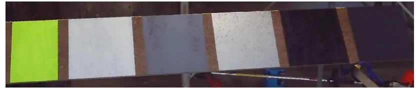
To test the effect of surface reflectivity on the TX5 a flat board was setup approximately 2.5m from the scanner facing approximately at the scanner. On the board were a number of different colour sections to ascertain the effect of colour and surface reflectivity on the accuracy and noise of the laser scanner. The different surface colours were (from right to left). Matt black, gloss black, silver, grey, white, and finally retro-reflective yellow (Figure 5).

Figure 5- Colour Test Board

25

3.3 Building Information Modelling Software

There are many building information modelling packages available on the market today. With offerings ranging from Graphisoft’s Archicad, Trimble’s Tekla, Bentley’s Buildings, Autodesk’s Revit, and many more it is very difficult to choose a package to use. When considering which package to use for this project I was looking for one that was going to be cheap to implement for the life of the project. It would also have to be IFC compliant, have plenty of assistance available online, and have powerful point cloud tools available.

I took the obvious choice in my opinion, Autodesk’s Revit. Not only does Autodesk offer free three year software licenses to students, have masses of online forums, tutorials and help desks. It is also IFC compliant and has a number of available plugins to handle point cloud data as well as its own point cloud engine.

Whilst researching software for this project and hardware requirements, it became very evident that when handling even medium to small size data sets that computer speed, processing cores, memory and solid state drives are very important handle the datasets in reasonable timeframes. Faro recommends 2.5GHz 64bit Multicore-processors, 16GB or more of RAM, and solid stated hard drives (Faro). For the sake of completeness, all point cloud processing will be carried out using on a system running the following:

 Intel Core i7-3770 CPU @3.40GHz (4 physical – 8 virtual processing cores)

 16GB Ram

 128GB Samsung 840 Pro Solid State Hard Drive

26

 Nvidia GeForce GT 640 Graphics Card

 Windows 8.1

3.4 The Sites

For this project, I have selected 3 different sites to try and analyse work flows and the suitability of terrestrial laser scanners in building information modelling. Each one is quite different and has been selected to present common scenarios that are given to a surveyor when carrying out surveys.

3.3.1 SITE 1–MODERN OFFICE BUILDING

The first site that has been chosen is a typical office building. It has been chosen due to its simple architecture, and the fact that it is a modern building, built to industry standards and it is expected that the walls, floors and ceilings will be relatively square and plumb. This will make extracting data from the point clouds a reasonably simple exercise.

3.3.2 SITE 2–INDUSTRIAL SHED

27

3.3.3 SITE 3–HOMESTEAD

The third and final site chosen for this project is an old stone homestead known as Strathneath. It was built circa 1860. It has thick stone walls, a full return verandah, a valleyed roof and lots of non-standard (in today’s terms at least) architecture, making it near on impossible to model accurately with more conventional survey methods. With pressed tin ceilings and many walls and features that are not quite square it should present quite a challenge to turn the laser scan point cloud into a suitable building information model. This site is also surrounded by a number of trees, and lush garden which will have the potential to make it difficult to get adequate scans of the outside of the building.

28

CHAPTER 4 – RESULTS AND ANALYSIS

4.1 Accuracy Testing

4.1.1 RANGING

Ranging testing went very simply, with the least squares adjustment carried out in the least squares module of Liscad and coordinates calculated for comparison. The results from angle readings can be found in Appendix 2 as an ISO Rounds report and the results from the least squares adjustment can be found in Appendix 3.

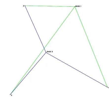
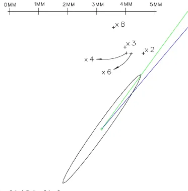
The traverse layout for the ranging test can be seen in Figure 7. In order to calculate a least squares adjusted solution, and to gain an orientation, the bearing from base 1 to sphere 1 was fixed, and all analysis done from here. This meant that distance only can be compared for sphere 1, and angle and distance can be compared on spheres 2 and 3.Diagrammatic representation of the error ellipse and the calculated position for each of the spheres from each accuracy setting can be seen in Figure 8 and Figure 9.

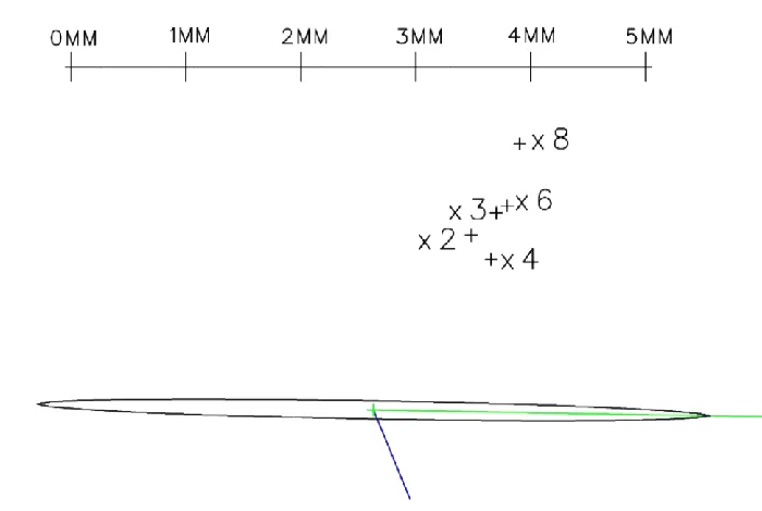
30 Figure 9. Angle Testing - Sphere 3

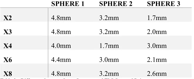
As can clearly be seen by the diagrams none of the calculated coordinates fell within the error ellipses from the total station observations. There are also no readily obvious patterns in the errors produced when the accuracy of the TLS is increased. Direct linear differences between the least square adjusted point and the points from the TLS can be seen in Table 2 - Difference between Least Squares and TLS Scanned Point.

SPHERE 1 SPHERE 2 SPHERE 3

X2 4.8mm 3.2mm 1.7mm

X3 4.8mm 3.2mm 2.0mm

X4 4.0mm 1.7mm 3.0mm

X6 4.4mm 3.0mm 2.1mm

X8 4.8mm 3.2mm 2.6mm

31

the TLS can be seen in Table 2 - Difference between Least Squares and TLS Scanned Point.

SPHERE 1 SPHERE 2 SPHERE 3

X2 4.8mm 3.2mm 1.7mm

X3 4.8mm 3.2mm 2.0mm

X4 4.0mm 1.7mm 3.0mm

X6 4.4mm 3.0mm 2.1mm

X8 4.8mm 3.2mm 2.6mm

Table 2 - Difference between Least Squares and TLS Scanned Point

Further analysis of the result, shows that the accuracy of the scanner is quite reasonable but in this case, not quite at the same accuracy as stated from Trimble. However, to ascertain if this was always the case more testing would be required. It is also clear from these results, that increasing the accuracy of the TLS does not necessarily increase the accuracy of points calculated from scanned spheres.

32

4.1.2 NOISE

Noise Testing at a Distance

Field testing for noise went without a hitch. In order to test the amount of noise evident when scanning the surface, initial results were gained by selecting a region within the scan point cloud and using the Scene software to get standard deviations of the distance scan points from the calculated plane. The results from this can be seen in (Figure 1010).

0.959

0.802 0.802

0.635

0.596

0.000 0.200 0.400 0.600 0.800 1.000 1.200

x2 x3 x4 x6 x8

Plan

e St

an

d

ar

d

De

viat

ion

(m

m

)

Quality

34

Noise Testing Up Close

Noise testing up close went exactly as expected, scans were carried out and data imported to Scene software. Once the data had been verified, the points within the cloud that were on the plane under scrutiny, were exported separately to the engineering calculation package Liscad SEE for modelling and comparison.

In Liscad, the point clouds which were not normalized to any particular plane were normalized so that the length and width of the board were the X and Y axes respectively and therefore the noise could be modelled and visually analyzed for any patterns by simply creating a terrain model and seeing if any patterns emerge. The results of this modelling can be seen in (Figure 11).

36

Visual analysis of this reveals a number of interesting observations in relation to noise created within the scan. Initial visual perusal indicates as the accuracy of the instrument is increased the noise that is evident in the scan decreases (as would be expected). It also initially appears that as the angle of incidence of the beam increases the amount of noise in the scan decreases significantly. Visual inspection of the models however does not tell the whole story. Point density also needs to be considered. To the far left of the scan, point spacing’s are approximately 1mm along the Y axis and as small as 0.5mm along the X axis. This resulted in a much higher impact of noise on the model when compared to the point spacing’s to the far right of the scan, where spacing in the Y axis was around 3mm and spacing of around 7mm along the X axis created a much lower point density.

Without further testing of the effect of the angle of incidence on the noise within a scan it is difficult to say with complete certainty what the effect is. However for the purposes of this project it can be concluded that the angle of incidence has no significant effect on the noise seen within a point cloud.

4.1.3 EDGE EFFECTS

37 Figure 12- Edge Effect - Accuracy x2

38 Figure 14- Edge Effect - Accuracy x4

Figure 15- Edge Effect - Accuracy x6

39

the scan. Further analysis of the number of erroneous points which don’t fall on either of the scanned planes confirms the results from the initial visual inspection. These results can be seen in Table 3 - Erroneous Points in Edge Effect Scan.

ACCURACY SETTING APPROX NUMBER OF POINTS

X2 1092

X3 1141

X4 1105

X6 1190

Table 3 - Erroneous Points in Edge Effect Scan

Analysis of the above table shows that the average number of erroneous points within the different scans is 1132. With the highest variance from the average only 5%, and the fact there is no clear reduction in erroneous points as the accuracy is increased. It is clear that the increase in accuracy of the TX5, has no significant effect on the edge effects evident within a TLS point cloud.

4.1.4 SURFACE REFLECTIVITY

Going into surface reflectivity, I initially had some preconceived notions about the results that were to be expected. Based on previous experiences with reflectorless electronic distance measurement techniques. The different surfaces were placed in roughly the order that the accuracy was expected. With the expected most accurate surface being the retro reflective yellow on the far left and the worst the matt black on the far right.

40

inspection of the three dimensional point cloud (Figure 163) quickly presented an obvious problem that the distance measured to the retro reflective tape was grossly in error and considerably outside of acceptable tolerances, in fact it was out by approximately 1m. Due to this large and unexpected error in the retro reflective surface results, it will be left out of any further result analysis in this portion.

Figure 16- 3D View of Colour Test Board Scan

White Grey

Silver

Matt Black Gloss Black

0 1 2 3 4 5 6 7

x1 x2 x3 x4 x6

Figure 17- Standard Deviation vs Colour and Quality

42

The results from this clearly show that there is a definite change in noise when either the colour (therefore reflectivity) being scanned or the accuracy of the scan varied. An observation that is supported by Boehler, Bordas Vicent and Marbs (2003). In respect to its application to BIM using TLS, the data from this test is rather inconclusive. However, it does give an indication of how a TLS operator or someone using the point cloud to create a BIM would need to be aware of the varying accuracies from differing surfaces, and that highly reflective surfaces such as signs, mirrors, and windows would need to be treated with extreme caution. If not deleted entirely from point clouds, however this will be investigated later on in the project when we look at the results from actual building scans.

4.2 The Building Scans

The process of scanning the buildings in this project was an extremely intensive learning process. With no prior experience with TLS, BIM or the associated software, it was very much a trial and error progression.

Following the accuracy testing carried out in the previous sections, it was deemed that the suggested settings in the software for the TX5 were generally an excellent balance between accuracy and speed. Hence these settings were used during all laser scans.

43

Artificial References

These include spheres, and checkerboard targets. They are placed around an area of a scan and are of a very specific nature, which makes them easily identifiable to the Scene software.

Natural References

Natural references include planes, slabs, pipes, corner points and rectangles. They are specific features that may be visible from a number of scanner locations that can then be used in place of artificial references to assist in registering scans in Scene (Reinhard Becker 2014).

Tensions

The term tension within Scene refers to the divergence in overall coordinate system between positioning of two relating reference objects in corresponding scans (Reinhard Becker 2014). It is an important value to the registration process, and is a good indicator of how well scans are being stitched together.

4.2.1 SITE 1:MODERN OFFICE BUILDING

The office building to be scanned was located at 6 Graves St in the township of Kadina, and is the local office of Mosel Steed, a medium sized surveying firm in South Australia.

44

In initial processing to start with I tried the auto registration available in Scene, allowing it to attempt to automatically recognize all the artificial targets that were placed in the office, and then place the scans automatically, by calculating between respective scans. The automatic target identification successfully identified all but one of the artificial targets in all 14 scans. It was a sphere located only a couple of metres from the TLS in scan number 4. This was quickly rectified by marking each of the missed targets within the software which then recognized the sphere.

Once all the targets were recognized, automatic placement of scans was attempted. This failed initially due to a lack of targets in a few key points. Scene managed to adequately tie together the first 10 scans and the final 3 scans as two individual clusters. However, there were insufficient artificial targets to adequately tie it all together. Further investigation revealed that scan number 10 (the one sitting out on its own) was an integral scan which should have tied both ends of the building together, with no overlap between the front and back parts of the office (being scans 12-14 and 1-11 respectively).

In order to try and tie all the scans together I then tried the automatic recognition of planes in the Scene software. It came up with quite a number of false planes, or ones that concerned me enough to not use this method initially.

45

Once this was done, an acceptable registration was achieved where all scans were successfully placed in reference to each other.

The entire registration process took approximately one hour and was relatively simple, whilst still allowing for some control and continuing quality control to be carried out during the process.

As a test to compare time of processing data for registration and placement of scans, the scans were reprocessed using the full automatic option, allowing Scene to automatically detect all spheres, checkerboard targets, planes, rectangles, edges, and corner points. It was then told to place all scans using fine registration in order to optimize tensions between all scans. This process was timed, to see how long it took the computer to process to use as a comparison for processing techniques in comparison to the semi-manual techniques described earlier. The automatic processing took approximately 22 minutes, and ultimately failed miserably. It initially split the scans into two separate scan clusters, but couldn’t tie them together. After a lot of looking through the results, and the dozens of natural references that scene had identified during the automated process. Trying to make these scans register with all the automatically recognized references had to be abandoned as it had taken considerably longer than using the semi-manual process described earlier.

46

Reflective Surfaces

Considering the results that became evident in the surface reflectivity testing in section 4.1.4 and the issues that became evident with the scanning of the retro-reflective yellow tape causing gross errors within the scan, it was clear that any highly reflective surfaces within the point cloud needed to be inspected and dealt with if errors were found to evident. In this case, the only highly reflective surface that fit this description was a mirror in the bathroom, which had only been partially scanned. Upon inspection, it was found that the mirror which was mounted directly to the wall had its scan points approximately 1.26 metres further away from the scanner than the wall itself. To deal with the scan points over the relatively small mirror, they were deleted from the scan entirely. This reflectivity issue causing problems will be dealt with again in the scanning of the Strathneath household, along with some illustrations of the problem.

4.2.2 SITE 2–INDUSTRIAL SHED

The industrial shed to be scanned was of a medium size, being approximately 20 metres long by 14 metres wide. It has 4.5 metre high walls with a gable roof. Its construction is with steel beams and columns, wooden purlins, and galvanized iron cladding, primarily, it is used as a small workshop and storage shed. As a result of its current usage it is very cluttered, and had quite a number of “in progress” projects, making it difficult for good coverage of all the areas inside with only a small number of scans.

47

approximately 368 million points. Of which 77 million were internal points and the remaining 291 million were external. Scanning took approximately 2 hours, and went relatively without a hitch.

Following the results from the attempted fully automatic registration from the office software, it was deemed that the similarly timed (although more labour intensive) semi-automatic registration process was to be adopted. As it provided a more hands on approach, and also means less time needs to be applied with respect to quality checking the registration and target recognition later, as this is carried out whilst marking the targets.

The scans were split into two separate clusters being inside and outside before being placed together for one homogenous point cloud. The inside point cloud was initially attempted to be registered with only the artificial targets that were placed around the shed which consisted of a total of 6 reference spheres and one checkerboard target. However, a problem presented when in a number of the scans some targets were either partially obscured from the scan, or were too far away from the scanner to give adequate points to be recognized at the resolution that had been scanned.

48

Following successful registration of the inside of the shed, attention was then turned to the scans that were carried out on the exterior. Initial attempts at registration involved only 10 spherical targets around the shed that were not a part of the inside scans, and also 4 of the spherical targets that were used for the inside scans so that the two clusters could eventually be tied together.

Initial thoughts were that the number of targets and their placement would have been adequate to carry out a successful registration. However it quickly became evident that this was not going to be the case. The reason for this is that a number of the smaller spherical targets were not close enough to some of the scanning stations, and hence were not able to be recognized by the software (due to the insufficient number of points scanned on their surface). This presented a challenge to try and get the scans to have an sufficient number of references to adequately tie the scans together. The solution was to look around the rest of the scans and locate enough planar surfaces within the scans to effectively tie them together.

Once the registration of both the inside and outside clusters were completed, the two clusters were placed together with Scene and resulted in mean tensions of less than 2mm.

49

not have been the case and may have resulted in the scans having to be carried out again.

4.2.3 SITE 3–HOMESTEAD

The homestead to be scanned was a relatively large single story house, with full return verandah. Excluding verandahs, the building is approximately 21m long by 12m wide. It has a central corridor, with a number of rooms running off both sides. The total number of scans was 34. This included 26 inside and 8 outside. This number could have been reduced by removing two scans inside which were not necessary to adequately scan all the rooms, but were added to get extra coverage in two of the larger rooms.

Registration of the scans within Scene on this particular site presented the greatest number of challenges within this project. Once extraneous points around the outside of the building were deleted from the data set, the scan totaled in excess of 2 billion points, of which 351 million were measured from the external scans, and the remainder were on the internal scans..

50

should be a very accurate model in this area of the house. However, issues arose with the registering of the scans of the separate rooms that came off the passage.

51

be forced to manually match, and then all internal scans managed to successfully register, with mean target tensions for all 26 scans at around 2mm or less.

Registration of the outside of the homestead was much simpler, with sight lines available down all four sides of the building, and the use of the reference spheres. It was a very simple process of marking the artificial targets within each of the scans and Scene then easily tied them all together with mean reference tensions below 1.5mm.

Once both the inside and outside clusters had been successfully registered, Scene was then used to tie both the clusters together. This went relatively smoothly with a total of 5 reference spheres tying the two clusters together, means tensions were 0.5mm for the two scans.

4.2.4 CONCLUSIONS

Whilst carrying out the scans a number of natural workflows and observations developed. Whilst analysing the work processes that were being carried out as each project scan developed, it became very evident how each problem that was faced and overcome could be applied to the final workflows in order to minimize problems in future large projects.

Artificial Reference Spheres

52

coordinate systems or for quality assurance checks. For more information see Appendix 4.

Whilst the targets are extremely accurate, care must be taken to place them in suitable positions for use in the registration process. The biggest problem that came about during the process of this project was that at times spheres were placed too far away from the scanner, and therefore unable to be recognized due to insufficient number of scan points falling on the sphere. In order to avoid this problem within the workflows of a business, it would be highly recommended to carry out some simple tests on any new scanners or targets to ascertain and tabulate both ideal and maximum distances for artificial targets. This could then be taken in the field for an operator to quickly refer to when placing targets to ensure there are no errors. It would simply be a resolution vs distance table for each type of reference. Indicating maximum distances to targets before recognition within the processing software, is outside of optimum range or unrecognizable all together. In the case of the TX5 used in this experiment. It appears that whilst this testing has not been done specifically (as it will vary between instruments and targets) it would be highly recommended and could potentially save a lot of problems with registration of scans in the office after leaving the field.

Large Sites

53

An excellent example that comes to mind, would be if one were to undertake a project such as providing a point cloud of an entire multi story hotel. It is very likely that there are quite a number of rooms with almost identical geometry, if not whole floors with potentially similar geometry. With narrow halls, doorways and corners in passages and rooms it would be highly likely that similar problems to those experienced when scanning the homestead would appear. In that references would appear to correspond with references that in reality they don’t correspond too.

The solution to this, prior to carrying out any scanning project, is to consider how scans will be clustered for processing once they have all been completed. Then once the scan project is underway, it would be beneficial to keep field notes on targets, and scan stations. It would also be highly recommended for any project where the scans did not form a closed loop (but had more of an open traverse) to be coordinated by some other form survey method such as total station or RTK GPS for quality assurance purposes.

Computer Power

A full analysis of the workflows involved in registering and working with the point clouds cannot be complete without a look at the processing power and process times required. As the saying goes, “Time is Money” and as surveyors we find ourselves constantly pushed for time, and any time saved in computer processing is money saved in the long term.

54

point cloud creation and point colourisation, all 8 logical cores within the CPU were operating at 100% for extended periods of time and memory usage was extremely high. In fact when creating the point cloud for the homestead, memory usage was up over 97% of the available 16 gigabytes. Such high usage of system resources renders the computer almost unusable for other tasks whilst these resource intensive processes run.

55

4.3 Building Information Modelling

Following the field work, testing, and registration of all the necessary laser scans. It was determined, with the testing and subsequent results that had been carried out to this point, that the laser scanners were still potentially suitable for building information modelling. As long as the data is treated with caution keeping consideration for the errors, and inherent attributes of the cloud produced from the laser scan as previously discussed.

4.3.1CONVERTING AND IMPORTING THE CLOUD

The first step in working with the point cloud in BIM is to have it converted to a format that the BIM software being used can handle. In previous versions of Autodesk’s Revit software it was necessary to use third party add-ons to handle point clouds. However in recent revisions Revit has added the ability to natively handle indexed point clouds within the Revit environment. The format required by Revit are either rcs or rcp files.

To enable the point cloud to be used within Revit each cloud was exported from Scene to the E57 file format. The E57 file format is a compact open source data exchange format that is vendor neutral and used for storing point clouds, images and metadata from 3D imaging systems such as the TLS used in this project (libE57: Software Tools for Managing E57 files 2010).

56

Once converted, the point cloud was inserted into Revit so that it may be used to create a building model.

4.3.2BUILDING THE MODEL

As stated earlier, to create the BIM the Revit add-on from Imaginit Technologies known as Scan to BIM was to be used. Scan to BIM has a number of tools available for BIM creation. However the main one that was to be investigated for its suitability was the wall creation tool.

In order to create a wall using the tools available within Scan to BIM, a user simply selects three points on a plane that they would like to recreate, and the tool automatically searches for points found within a tolerance as set by the user to fall within that plane and it reports back on the points found. Once the plane has been found, the user then selects what type of wall to create, hence specifying its thickness and then it’s done.

57

discovered that the most efficient and accurate way to determine wall thickness, was to measure from a cross section of the point cloud. This was then used to determine the wall thickness, and then the assumption was made that the wall had an even thickness throughout each plane.

The other major problem inherent in this work process is that it assumes walls are perfectly flat. Whilst this is generally true in modern buildings such as the office scanned, it is obviously not the case in buildings such as the homestead in this project. Therefore, walls created using this work process will have inherent inaccuracies in their model. Whilst, measurements could be made on the point cloud directly, this is not ideal due to the large size of point cloud datasets, and large computing power required for handling such datasets.

4.3.3ACCURACY OF THE MODEL

To compare accuracy of the building models, a number of rooms in sites 1 and 3 were measured using tape measures and laser distance meters. A number of both diagonal room measurements and cross-sectional measurements were taken for comparison. The dimensions chosen to be compared varied, between measurements that had walls that were measured from the same scan, to others where some walls had been created from scans on the far side of the wall.

Dimensions that were to be compared were also measured in the Scene software in order to compare results for the plane fit algorithms in both Scene and Scan to Bim. The results can be seen tabulated in (Figure 14)

58

but one of the compared measurements falling under 10mm, and an average difference of 4mm, it is clear that the TLS accuracy and the subsequent registration are extremely accurate and producing the results that would be expected given the specs of the TLS. In fact the only result over 10mm, can be accounted for as the measurement that is being compared, is in a room where the distance comparison used in the laser scan data was measured at approximately 2m above the floor level. due to a door blocking part of the laser scan, whereas the tape measured distance was measured approximately 1m above the floor. With the varying wall thicknesses and walls not being square, this result can therefore be discounted. This brings the average difference in distance comparisons to only 3mm.

59

CHAPTER 5 – CONCLUSION

The purpose of this project was to ascertain the suitability of TLS in BIM. Whilst this project’s ultimate conclusion is that TLS are indeed suitable for BIM it should be made clear that they need to be treated with caution. It is very important to remember when producing point clouds and building models from TLS that they have inherent errors due to the way in which they work and are produced. All of these errors have been discussed in earlier sections.

The initial aims of this project were to investigate not only the suitability of TLS in BIM, but to also develop workflows for extracting geometric and structural information from laser scanning point cloud data. The workflows have come a long way, but as stated in many online blogs and websites, the reconstruction of structural and geometric information is an extremely complex and difficult group of tasks. Whilst it is relatively simple to recreate structural elements such as walls, floors and ceilings from point clouds. It is a much more difficult task to recreate more complex components of buildings such as columns, windows, doors, and fixtures.

60

5.1 Further Work

61

REFERENCES

Bazjanac, V & Crawley, DB 1997, 'The implementation of industry foundation classes in simulation tools for the building industry'.

BIMForum 2013, Level of Development Specification.

Boehler, W, Bordas Vicent, M & Marbs, A 2003, 'Investigating laser scanner accuracy', The International Archives of Photogrammetry, Remote Sensing and Spatial Information Sciences, vol. 34, no. Part 5, pp. 696-701.

Campbell, RJ & Flynn, PJ 2001, 'A survey of free-form object representation and recognition techniques', Computer Vision and Image Understanding, vol. 81, no. 2, pp. 166-210.

De Luca, L, Véron, P & Florenzano, M 2006, 'Reverse engineering of architectural buildings based on a hybrid modeling approach', Computers & Graphics, vol. 30, no. 2, pp. 160-76.

Epstein, E 2012, Implementing successful building information modeling, Artech

House, Boston,

<http://ezproxy.usq.edu.au/login?url=http://site.ebrary.com/lib/unisouthernqld/Doc?i d=10583832>.

Faro FARO Laser Scanner Software, viewed 07/09/2014, < http://www.faro.com/en-us/products/faro-software/scene/system-requirements#main>.

Faro 2013, 'Laser Scanner Focus 3D- Faro', p. 4.

Leica-Geosystems 2013, Leica ScanStation P20, Heerbrugg, Switzerland, <

http://hds.leica- geosystems.com/downloads123/hds/hds/ScanStation_P20/brochures-datasheet/Leica_ScanStation_P20_DAT_en.pdf>.

libE57: Software Tools for Managing E57 files, 2010, 3D Imaging System File Format Committee, viewed 18/10/14, <http://www.libe57.org/>.

62

Pu, S & Vosselman, G 2006, 'Automatic extraction of building features from terrestrial laser scanning', International Archives of Photogrammetry, Remote Sensing and Spatial Information Sciences, vol. 36, no. 5, pp. 25-7.

Reinhard Becker, JG, Susanne Schweigert, Daniel Flohr, Stefan Bertele, Joachim Vollrath, Thomas Hermle 2014, Scene 5.2, Faro Technologies.

Riegl 2013, Riegl VZ-4000,

< http://www.riegl.com/uploads/tx_pxpriegldownloads/10_DataSheet_VZ-4000_23-09-2013.pdf>.

Steel, J, Drogemuller, R & Toth, B 2012, 'Model interoperability in building information modelling', Software & Systems Modeling, vol. 11, no. 1, pp. 99-109.

Tang, P, Huber, D, Akinci, B, Lipman, R & Lytle, A 2010, 'Automatic reconstruction of as-built building information models from laser-scanned point clouds: A review of related techniques', Automation in Construction, vol. 19, no. 7, pp. 829-43.

Trimble 2012, Datasheet - Trimble TX5 Scanner,

< http://trl.trimble.com/dscgi/ds.py/Get/File-628869/022504-122_Trimble_TX5_DS_1012_LR.pdf>.

Tucker, C 2002, 'Testing and verification of the accuracy of 3D laser scanning data', in Symposium on Geospatial Theory, Processing and Applications, Ottawa:

proceedings of theSymposium on Geospatial Theory, Processing and Applications, Ottawa.

Vandezande, J, Krygiel, E & Read, P 2013, Mastering Autodesk Revit Architecture 2014, John Wiley & Soncs Inc, Indianapolis, Indiana.

ENG 4111/ENG4112 Research Project

PROJECT SPECIFICATION

FOR: BRENTON LIGHT

TOPIC: Terrestrial laser scanning for building information model (BIM) development and application

SUPERVISOR: Dr Zhenyu Zhang

SPONSORSHIP: Ultimate Positioning, Mosel Steed

PROJECT AIM: To investigate the use of terrestrial laser scanning for building information modelling as an alternative to conventional survey techniques.

PROGRAMME: Issue A, 7th April 2014

1. Research background information relating to building information modelling

2. Research background information relating to Terrestrial laser scanners 3. Analyse suitability of laser scanners in building information modelling. 4. Design workflows to implement terrestrial laser scanning in

as-constructed data capture by taking on a real world project. 5. Analyse workflows and ascertain whether they may be viable and

necessary in today’s market. If time permits:

B

ISO Rounds Report

Project BAL ANGLE TEST Date 19.06.2006

Instrument Trimble S6 3 DR 300+ Distance unit Metres

Serial Number 13367 Angle unit DMS Degrees

Firmware

Version R12.5.37 Temperatureunit Celsius

Pressure unit hPa Trimble Survey Controller v12.49

Project Properties

Latitude Origin ?

Longitude Origin ?

False Easting ?

False Northing ?

Scale 1.000000

Datum Transformation

Type No Datum

Earth radius ?

Flattening ?

Scale ? ppm

Corrections

Distances as Ground

South azimuth No

Grid Orientation Increasing NE

Magnetic Declination 0°00'00"

Neighborhood

Adjustment Off

Instrument Station

Stationing Type Station Setup

Atmospheric Settings

Station BASE Temperature 18.0°C

Code Pressure 1011.4hPa

Instrument

Horizontal Circle

Mode Set To Azimuth

Standard Deviations

Hz 0°00'03"dms

V 0°00'03"dms

EDM constant 3mm

EDM ppm 2ppm

Centering Error 0mm

Backsight Points

Point Name Easting Northing Elevation

1 5003.1965 9991.2177 98.4817

Measurements

Point Name Code SD [m] HA [dms] VA [dms] th [m] PC [mm]

1 SPHERE 9.4689 160°00'00" 99°13'32" 0.0000 -34 1 SPHERE 9.4690 339°57'36" 260°46'10" 0.0000 -34 1 SPHERE 9.4684 160°00'00" 99°13'25" 0.0000 -34 1 SPHERE 9.4674 339°59'55" 260°46'15" 0.0000 -34

Result

Coordinates Std.Dev. Std.Dev.

Easting 5000.0000 ?m Orientation 0°01'12" ?

Northing 10000.0000 ?m Scale 1.000000 ?

Elevation 100.0000 ?m

Multiple Rounds

1. Horizontal Angles

1 2 3 4 5 6 7 8 9 10

Station Target Face 1 Face 2 _L1+L2Mean _ReducedMean _{of all sets}Mean out Diff._(D) Res._(R) R²

dms dms dms dms dms sec sec sec²

BASE 1 160°00'00" 339°57'36" 159°58'48" 0°00'00" 0°00'00" 00.0 -29.7 879.382 2 213°30'41" 33°32'00" 213°31'20" 53°32'32" 53°33'17" 44.8 15.1 228.027 3 270°59'26" 91°00'02" 270°59'44" 111°00'56" 111°01'40" 44.2 14.6 211.813

29.7

1 160°00'00" 339°59'55" 159°59'57" 0°00'00" 00.0 29.7 879.382 2 213°33'27" 33°34'31" 213°33'59" 53°34'02" -44.8 -15.1 228.027 3 271°02'04" 91°02'40" 271°02'22" 111°02'24" -44.2 -14.6 211.813

-29.7

Sum 00.0 2638.444

Number of sets 2

Number of targets 3

Std.Dev. of a direction measured in

both faces 36.3 sec

Std.Dev. of a direction averaged over 2

sets 25.7 sec

2. Vertical Angles

1 2 3 4 5 6 7 8 9

Station Target Face 1 Face 2 _IndexV- _L1+L2Mean _{of all sets}Mean out Res._(R) R²

dms dms sec dms dms sec sec²

BASE 1 99°13'32" 260°46'10" -09.1 99°13'41" 99°13'38" -03.1 09.735 2 92°48'39" 267°10'55" -13.2 92°48'52" 92°48'47" -05.1 25.621 3 91°24'26" 268°34'59" -17.3 91°24'43" 91°24'41" -02.7 07.102

-39.6

1 99°13'25" 260°46'15" -09.6 99°13'35" 03.1 09.735 2 92°48'22" 267°10'58" -20.1 92°48'42" 05.1 25.621 3 91°24'19" 268°35'03" -19.0 91°24'38" 02.7 07.102

-48.7

Sum 00.0 84.915

Mean Index Correction -14.7 sec

Number of sets 2

Number of targets 3

Number of degrees of freedom 3

Std.Dev. of a vertical angle measured

in both faces 05.3 sec

Std.Dev. of a vertical angle averaged

over 2 sets 03.8 sec

3. Distances

1 2 3 4 5 6 7 8 9 10

Station Target Face 1 Face 2 out of allMean sets

Res.

(R1) Res.(R2) Sum(R²) Std.Dev Std.Dev.Mean

m m m mm mm mm² mm mm

BASE 1 9.4689 9.4690 9.4684 -0.5 -0.6 0.59 0.8 0.5

2 11.5190 11.5196 11.5195 0.4 -0.1 0.20 0.3 0.2

3 4.9158 4.9159 4.9157 -0.2 -0.2 0.09 0.3 0.2

1 9.4684 9.4674 0.0 1.1 1.13

2 11.5194 11.5198 0.1 -0.4 0.15

3 4.9152 4.9157 0.4 0.0 0.20

Sum 0.31 -0.31 2.36

Number of sets 2

Number of targets 3

Std. Dev. of a distance measured in 1 face - see column 9 above

Std. Dev. of the mean of all sets - see column 10 above

Std. Dev. for all distances (1 obs only) 0.5 mm

Std. Dev. for all distances (mean) 0.4 mm

4. Averaged Data Sets

Point

Name Code HA VA SD ih/th PC Temp[°C] Press[hPa]

BASE 0.000

1 SPHERE 0°00'00" 99°13'38" 9.4684 0.000 -34.0 18.0 1011.4 2 SPHERE 53°33'17" 92°48'47" 11.5195 0.000 -34.0 18.0 1011.4

3_SPHERESMAL111°01'40" 91°24'41" 4.9157 0.000 -34.0 18.0 1011.4

Point

Name Code Az VA SD ih/th

BASE 0.000

1 SPHERE 160°00'00" 99°13'38" 9.4684 0.000 2 SPHERE 213°33'17" 92°48'47" 11.5195 0.000

3_SPHERESMAL271°01'40" 91°24'41" 4.9157 0.000

Point

Name Code Az HD VD

BASE

1 SPHERE 160°00'00" 9.346 -1.518 2 SPHERE 213°33'17" 11.506 -0.565

3_SPHERESMAL271°01'40" 4.914 -0.121

Point

Name Code Easting Northing Elevation

BASE 5000.0000 10000.0000 100.0000

1 SPHERE 5003.1954 9991.2167 98.4816 2 SPHERE 4993.6404 9990.4123 99.4334

3 SMAL

SPHERE 4995.0830 10000.0907 99.8770

Instrument Station

Stationing Type Standard Resection

Atmospheric Settings

Station BASE2 Temperature 18.0°C

Code Pressure 1011.4hPa

Instrument

Height 0.000 RefractionConst. 0.142

Mode Set To Azimuth

Standard Deviations

Hz 0°00'03"dms

V 0°00'03"dms

EDM constant 3mm

EDM ppm 2ppm

Centering Error 0mm

Backsight Points

Point Name Easting Northing Elevation

1 5003.1965 9991.2177 98.4817

2 4993.6405 9990.4117 99.4347

Measurements

Point Name Code SD [m] HA [dms] VA [dms] th [m] PC [mm]

1 SPHERE 7.2073 122°00'48" 98°59'55" 0.0000 -34 2 SPHERE 5.7783 217°32'28" 91°44'50" 0.0000 -34

Residuals

Point Name Code Station_[m] Offset [m] delta Hz_[dms] delta E_[m] delta N_[m] delta El_[m]

1 SPHERE 0.0006 0.0000 -0°00'00" 0.0005 -0.0003 -0.0009

2 SPHERE 0.0005 0.0000 0°00'00" -0.0003 -0.0004 0.0009

Result

Coordinates Std.Dev. Std.Dev.

Easting 4997.1600 0.001m Orientation 0°00'00" 0°00'15"

Northing 9994.9917 0.000m Scale 1.000000 ?

Elevation 99.6099 0.001m

Multiple Rounds

1. Horizontal Angles

1 2 3 4 5 6 7 8 9 10

Station Target Face 1 Face 2 _L1+L2Mean _ReducedMean _{of all sets}Mean out Diff._(D) Res._(R) R²

dms dms dms dms dms sec sec sec²

BASE2 2 217°32'13" 37°33'43" 217°32'58" 0°00'00" 0°00'00" 00.0 24.0 573.749 3 337°51'26" 157°51'58" 337°51'42" 120°18'44" 120°18'09" -35.8 -11.9 141.128 1 122°01'51" 302°02'07" 122°01'59" 264°29'01" 264°28'25" -36.0 -12.1 145.765

-24.0

2 217°33'11" 37°33'42" 217°33'27" 0°00'00" 00.0 -24.0 573.749 3 337°49'00" 157°52'59" 337°50'59" 120°17'33" 35.8 11.9 141.128 1 122°01'08" 302°01'23" 122°01'16" 264°27'49" 36.0 12.1 145.765

Sum 00.0 1721.283

Number of sets 2

Number of targets 3

Number of degrees of freedom 2

Std.Dev. of a direction measured in

both faces 29.3 sec

Std.Dev. of a direction averaged over 2

sets 20.7 sec

2. Vertical Angles

1 2 3 4 5 6 7 8 9

Station Target Face 1 Face 2 _IndexV- _L1+L2Mean _{of all sets}Mean out Res._(R) R²

dms dms sec dms dms sec sec²

BASE2 2 91°44'50" 268°14'33" -18.7 91°45'08" 91°45'02" -06.2 38.477 3 87°13'09" 272°46'17" -17.1 87°13'26" 87°13'24" -02.1 04.263 1 99°00'18" 260°59'24" -08.9 99°00'27" 99°00'24" -02.6 06.922

-44.7

2 91°44'54" 268°15'02" -01.8 91°44'56" 06.2 38.477 3 87°13'28" 272°46'45" 06.4 87°13'22" 02.1 04.263 1 99°00'09" 260°59'25" -13.3 99°00'22" 02.6 06.922

-08.7

Sum 00.0 99.323

Mean Index Correction -08.9 sec

Number of sets 2

Number of targets 3

Number of degrees of freedom 3

Std.Dev. of a vertical angle measured

in both faces 05.8 sec

Std.Dev. of a vertical angle averaged

over 2 sets 04.1 sec

3. Distances

1 2 3 4 5 6 7 8 9 10

Station Target Face 1 Face 2 out of allMean sets

Res.

(R1) Res.(R2) Sum(R²) Std.Dev Std.Dev.Mean

m m m mm mm mm² mm mm

BASE2 2 5.7780 5.7788 5.7784 0.4 -0.4 0.30 0.4 0.3

3 5.5128 5.5122 5.5123 -0.5 0.1 0.25 0.5 0.3

1 7.2078 7.2079 7.2076 -0.2 -0.3 0.10 0.3 0.2

2 5.7781 5.7786 0.3 -0.2 0.14

1 7.2073 7.2075 0.3 0.1 0.11

Sum 0.10 -0.10 1.29

Number of sets 2

Number of targets 3

Number of degrees of freedom 3

Std. Dev. of a distance measured in 1 face - see column 9 above

Std. Dev. of the mean of a