Structural Dynamics of Complex Molecules by Ultrafast Electron Diffraction: Concepts, Methodology and Applications

Full text

(1)Structural Dynamics of Complex Molecules by Ultrafast Electron Diffraction: Concepts, Methodology and Applications. Thesis by. Ramesh Srinivasan. In partial fulfillment of the requirements for the degree of Doctor of Philosophy. California Institute of Technology Pasadena, California 2005 (Defended December 1, 2004).

(2) ii. © 2005 Ramesh Srinivasan All Rights Reserved.

(3) iii. Dedicated with love and gratitude to. Bhagawan Sri Sathya Sai Baba and to my dearest parents. Aruna and N.V. Srinivasan.

(4) iv. Acknowledgements In my native land of India, every person is regarded as having two births–the first, birth into the physical world, and the other, birth into the world of knowledge. Indian tradition emphasizes that for the former birth, we are eternally indebted to our parents, and for the latter, we are ever beholden to our teacher. It is in that spirit of my ancestors that I write these words of gratitude to my teacher and mentor, Prof. Ahmed Zewail. The human language, while a wondrously marvelous gift, often fails at times such as these to adequately express the whole gamut of one’s emotions. Yet, standing as I am at the end of a long and arduous period of graduate school, it is but natural that I seek to acknowledge his profound influence on my growth as a scientist and as a human being. My entry into the Zewail group came about under very unusual circumstances, the details of which will have to wait for another day. Over the course of my studentship, I have been struck and inspired by his passion for science and his insatiable curiosity about the natural world. The award of the Nobel Prize in 1999 was certainly one of the high points of my tutelage under him. I am reminded of an anecdote that Isidor Isaac Rabi once shared, “My mother made me a scientist without ever intending to. Every other Jewish mother in Brooklyn would ask her child after school, ‘So? Did you learn anything today?’ But not my mother. ‘Izzy,’.

(5) v. she would say, ‘did you ask a good question today?’ That difference–asking good questions–made me become a scientist.” It has been my singular fortune to learn from Prof. Zewail the art of asking the right questions. I have enjoyed our numerous discussions on the history of science, on the role of science and technology in bridging the gap between the ‘haves’ and the ‘havenots’, on the cultural mores of our respective ancient civilizations, and on the art of communicating science to non-scientists and especially to young, budding scientists. While he has been a wonderful teacher, I hope I have been a worthy disciple. I am also grateful to his wife, Dema, and his sons, Hani and Nabeel, for giving me a home away from home, for many wonderful evenings of joy and laughter. I have had the privilege of working with a team of brilliant and superbly accomplished colleagues over the years, not only in the diffraction sub-group but also in the larger Zewail group. My earliest foray into femtochemistry, albeit for an all-too-brief period, was with Chaozhi Wan and Spencer Baskin. I was soon lured into the challenging world of ultrafast diffraction. It was here that Udo Gomez and Vladimir Lobastov, two remarkable postdoctoral scholars, took me under their wings and taught me all I know about diffraction and equipment design. Vladimir, in particular, has been a tremendous mentor and colleague, and I will always cherish the experience of working with and learning from him. Hyotcherl Ihee and Jim.

(6) vi. Cao, both members of the UED-2 team, shared generously from their wealth of experience and honed my skills in the theoretical analysis of the molecular diffraction signatures. The UED-3 team has, over the years, benefited from many outstanding personnel, each of whom brought their unique perspective and expertise to bear upon this discipline. Chong-Yu Ruan, Boyd Goodson, Jon Feenstra, Sang Tae Park, and Shoujun Xu have all been an integral part of this exciting endeavor. Jon and I have worked particularly closely for nearly 4 years, and it has been a wonderful experience having him as a colleague and as a friend. All of the work that is discussed in this dissertation bears their unmistakable imprint, and to each one of them, I owe many thanks. All present and former members of the Zewail group not only provided me with a stimulating intellectual ambience, but they have also been wonderful friends. I can never forget the amazing secretaries we have had over the years, who made life in the sub-basement far easier than it otherwise might have been. Mary Sexton, Sylvia Jacoby, Janet Davis, and De Ann Lewis have all been an inexhaustible source of cheer and comfort. I also wish to thank all the faculty of the Chemistry and Chemical Engineering Division for their formal and informal guidance over the years. In particular, I wish to thank Prof. George Gavalas for his mentorship during my master’s thesis. Prof. Vince McKoy always evinced great personal interest.

(7) vii. in my research, and his constant encouragement has been one of the abiding memories of my graduate career. The National Science Foundation and the Air Office of Scientific Research are gratefully acknowledged for their generous financial support of this work. To my parents, I owe all that I am and hope to be. Their unstinting support, words of comfort and wisdom, and their unshakable belief in me helped me push myself harder when I didn’t think I could do any better. This dissertation is more a testimony to their love than to my abilities. To Bhagawan Sri Sathya Sai Baba, my dearest friend and guide, I offer this labor of love in a spirit of humble dedication.. Ramesh Srinivasan Pasadena, California November 23, 2004.

(8) viii. Abstract The central theme in ultrafast electron diffraction (UED) is the elucidation of the structural dynamics of transient molecular entities. With properly timed sequences of ultrafast electron pulses, it is now possible to image complex molecular structures in the four dimensions of space and time with resolutions approaching 0.01 Å and 1 ps, respectively. Reaching this spatiotemporal resolution on the atomic scale has been the driving force behind the development and application of the third generation UED instrument–the subject of this dissertation. The current state-of-the-art in resolutions and sensitivity, together with theoretical advances, has made possible the direct determination of transient structures, leading to studies of diverse molecular phenomena hitherto not accessible to other techniques. By freezing structures on the ultrafast timescale, we are able to develop concepts that correlate structure with dynamics. Examples include structure-driven radiationless processes, dynamics-driven reaction stereochemistry, and nonequilibrium structures exhibiting negative temperature, bifurcation, or selective energy localization in bonds. These successes in the studies of complex molecular systems, even without heavy atoms, establish UED as a powerful method for mapping out temporally changing molecular structures in chemistry, and potentially, in biology..

(9) ix. Table of Contents. Acknowledgements…………………………………………………………...……iv Abstract……………………………………………………………..………….….viii List of Figures…………………………………………………...………………..xiv List of Schemes……………………………………………………..………..…xxiii List of Tables……………………………………………………..……………..xxiv 1. Introduction…………………………………………………………………………1 Figures……………………………………………………………………...10 References...........................................................................................12 2. UED Theory……………………………………………………………………….18 2.1. Introduction........................................................................................18. 2.2. The Diffraction-Difference Method: Transient Structures…………22. 2.3. Ground-State Structures...................................................................27. 2.4. Structure Search and Refinement.....................................................28 Figures……………………………………………………………………...32 References...........................................................................................35. 3. Third Generation UED Instrumentation……………………………………..36 3.1. Introduction........................................................................................36. 3.2. Femtosecond Laser System...............................................................37. 3.3. Vacuum Chambers and Molecular Beams........................................39. 3.4. Electron Gun.......................................................................................40. 3.5. CCD Camera System.........................................................................41. 3.6. Time-of-Flight Mass Spectrometer....................................................44 References...........................................................................................45 Figures……………………………………………………………………...46.

(10) x. 4. UED Methodology……………………………………………………………….64 4.1. Introduction………………………………………………………………64. 4.2. Streaking: Electron Pulse Characterization.....................................65. 4.3. Clocking: Zero of Time………………………………………..……….....70. 4.4. Temporal and Spatial Overlap: Velocity Mismatch……..…………..73. 4.5. Calibration of CCD Camera…………………………………..………...76. 4.6. CCD Image Processing……………………………………........……….76. 4.7. Normalization of Time-Dependent Diffraction Signals………..…...81. 4.8. Analysis of 1D Diffraction Data: Ground-State Structures……..…82. 4.9. Time-Resolved Experiments: The Diffraction-Difference Method……………………………………………………………………...84. 4.10. Least-Squares Fitting........................................................................88. 4.11. Estimation of Spatial Coherence.......................................................90 References...........................................................................................91 Figures…………………………………………………………………..….92. 5. Reactive Intermediate Structures: A Case Study…………………..……...111 5.1. Introduction......................................................................................111. 5.2. Experimental………………………………………………………........114. 5.3. Results and Discussion A. Ground-State Structures of C2F4I2……………………...………..115 B. Structural Dynamics of the C2F4I2 Reaction.............................116 C. Structural Change, Intermediate to Product: The C2F4I → C2F4 + I Process………………….................................................122 D. Structure of the C2F4I Radical Intermediate……………………124. 5.4. Conclusions………………………………………………………………132 Figures…………………………………………………………………….133 References……………………………………………………….……….146.

(11) xi. 6. Dark Structures in Nonradiative Processes…………………..…………….148 6.1. Introduction………………………………………………………………148. 6.2. Ground-State Structures A. Pyridine………………………………………………………….…..158 B. 2-Picoline……………………………………………………..……..160 C. 2,6-Lutidine…………………………………………………………160. 6.3. Transient Structures A. Pyridine……………………………………………………………...161 B. 2-Picoline…………………………………………………………....165 C. 2,6-Lutidine………………………………………………………....166. 6.4. Photochemistry A. Pyridine…………………………………………………………...…166 B. 2-Picoline………………………………………………………..…..174 C. 2,6-Lutidine…………………………………………………...…….177. 6.5. Photophysics……………………………………………………………..178. 6.6. Conclusions……………………………………………………………....182 Figures…………………………………………………………………….184 References……………………………………………………………..…210. 7. Non-Equilibrium Structures………………………………………..…………216 7.1. Introduction………………………………………………………………216. 7.2. Concepts of Equilibrium vs. Non-equilibrium Structures………...217. 7.3. Experimental Methodology…………………………………………….220. 7.4. Data Processing and Analysis A. Background Subtraction……………………………………….…220 B. Generation of “Product-Isolated” Curves from Diffraction Difference Signals.......................................................................221 C. Novel Aspects of the Product Structure Analysis Used for “Hot” HT Product........................................................................224.

(12) xii. D. The Generalized Monte Carlo Method: A Complementary Analysis.......................................................................................229 7.5. Results and Discussion A. Ground States of CHT and CHD................................................231 B. Structural Dynamics of CHT………………………………….....232 C. Structural Dynamics of CHD………………………………….…234. 7.6. Review of Previous Studies in Light of Our UED Results A. The Resonance Raman Studies of Mathies and co-workers…243 B. The Initial Work of Sension and co-workers……………………246 C. The Work of Fuss, Kompa, and co-workers……………………248. 7.7. Implications of UED Studies on Understanding IVR……………..251. 7.8. Conclusions………………………………………………………………258 Figures…………………………………………………………………….259 References………………………………………………………………..277. 8. Conformational Dynamics on Complex Energy Landscapes…………......280 8.1. Introduction………………………………………………………………280. 8.2. Methodology…………………………………………………………...…282. 8.3. Structure Refinement…………………………………………………..283. 8.4. DFT Calculations………………………………………………………..284. 8.5. Monte Carlo Global Structural Optimization…………………...….285. 8.6. Results and Discussion A. Structures of Cope Rearrangement………………………….….285 B. Ring Opening Reactions…………………………………………..289 C. The Observation of Non-equilibrium Configurations in OT….291. 8.7. Conclusions…………………………………………………………..…..299 Figures…………………………………………………………………….301 References……………………………………………………….........….313.

(13) xiii. 9. Hydrogen-Bonding in Acetylacetone……………………………..……….….315 9.1. Introduction…………………………………………………………..….315. 9.2. Experimental…………………………………………………………….318. 9.3. Ground State………………………………………………………….….318. 9.4. Structural Dynamics…………………………………………...……….322. 9.5. Results and Discussion…………………………………………………323. 9.6. Conclusions…………………………………………………………..…..329 Figures…………………………………………………………………….330 References………………………………………………………………..343. 10. Conclusions and Future Directions……………………..……………………347 Figures…………………………………………………………………….351 References………………………………………………………………..352.

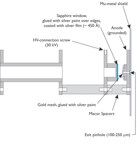
(14) xiv. List of Figures 1-1. Example of diffraction with two scattering centers................................ 10. 1-2. The UED experiment............................................................................... 11. 2-1. Concept of ultrafast electron diffraction ................................................. 32. 2-2. The diffraction-difference method ........................................................... 33. 2-3. Isolation of transient species through choice of tref ................................ 34. 3-1. Third-generation UED-3 apparatus........................................................ 46. 3-2. Layout of beam path for the femtosecond laser pulses .......................... 47. 3-3a Schematic front view of the UED-3 apparatus....................................... 48 3-3b Schematic side view of UED-3 apparatus............................................... 49 3-4. Schematic of UED-3 electron gun assembly ........................................... 50. 3-5. Detailed view of the electron generation and acceleration assembly .................................................................................................. 51. 3-6. Equipotential lines in extraction region of electron gun........................ 52. 3-7. Detailed view of magnetic lens assembly ............................................... 53.

(15) LIST OF FIGURES. xv. 3-8. Detailed view of the electron streaking and deflection assembly.......... 54. 3-9. UED-3 detector assembly ........................................................................ 55. 3-10 Individual components of the custom-made detector assembly............. 56 3-11 Photographs of selected detector components ........................................ 57 3-12 Schematic of time-of-flight mass spectrometry apparatus .................... 58 3-13 The linear TOF-MS chamber .................................................................. 59 3-14 Acceleration and detector assembly for time-of-flight apparatus.......... 60 3-15 Geometry of time-of-flight mass spectrometer ....................................... 61 3-16 Arrangement and synchronization of electrical pulses in TOF-MS ...... 62 3-17 Typical mass spectrum obtained in the TOF-MS apparatus ................. 63 4-1. Calibration of electron gun via streaking experiments.......................... 92. 4-2. Typical X-Y profile of the nearly circular electron beam ....................... 93. 4-3. Results of in situ streaking experiment for electron pulse measurement ........................................................................................... 94. 4-4. Calibration of electron pulse width ......................................................... 95. 4-5. Improvement in electron gun performance ............................................ 96.

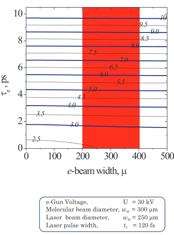
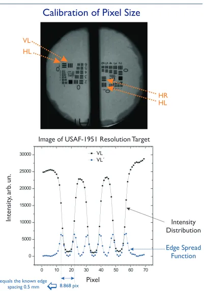
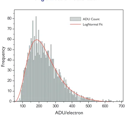
(16) LIST OF FIGURES. xvi. 4-6. Pulse-to-pulse stability of the electron gun ............................................ 97. 4-7. Lensing experiment to determine in situ the zero-of-time..................... 98. 4-8. Photoionization-induced ‘lensing’ effect for measuring time-zero ......... 99. 4-9. Geometry of crossed-beam experiment ................................................. 100. 4-10 Angular dependence of temporal broadening due to velocity mismatch ............................................................................................... 101 4-11 Overall temporal resolution (including velocity mismatch) as a function of spatial and temporal width of the electron pulses ............ 102 4-12 Calibration of pixel size on phosphor screen using Group 0, Element 1 of the USAF-1951 resolution target.................................... 103 4-13 Determination of mean pixel size on phosphor screen......................... 104 4-14 Modulation Transfer Function for the ICCD camera........................... 105 4-15 Calibration of single electron events on the detector ........................... 106 4-16 Inverse atomic ratio method.................................................................. 107 4-17 Processing procedure for 2-D diffraction images and ground-state data analysis.......................................................................................... 108 4-18 Diffraction-difference analysis for time-resolved experiments ............ 109.

(17) LIST OF FIGURES. xvii. 4-19 Divergence of electron beam.................................................................. 110 5-1. Ground-state molecular diffraction image of C2F4I2 ............................ 135. 5-2. Refined ground-state structure of C2F4I2 .............................................. 136. 5-3. Time-resolved 2D diffraction-difference images of C2F4I2 ................... 137. 5-4. Effect of Fourier filtering on raw diffraction-difference curves ........... 138. 5-5. Time-resolved structural changes in the elimination of iodine from C2F4I2 ............................................................................................. 139. 5-6. Time-resolved structural changes involving only the C2F4I → C2F4 + I contribution to the diffraction-difference signal .................... 140. 5-7. Time dependence of the formation of C2F4 molecules from the decay of C2F4I transient structures ...................................................... 141. 5-8. Structural determination of the transient C2F4I intermediate ........... 142. 5-9. Refinement of the C2F4I radical structure ............................................ 143. 5-10 Complete structural determination of the C2F4I2 elimination reaction .................................................................................................. 144 6-1. Ground-state molecular diffraction image of pyridine ......................... 185. 6-2. Comparison between experimental and refined theoretical sM(s) and f(r) curves for ground-state pyridine ............................................. 186.

(18) LIST OF FIGURES. xviii. 6-3. Refined ground-state structural parameters of pyridine ..................... 187. 6-4. Ground-state molecular diffraction image of picoline .......................... 188. 6-5. Refined ground-state structural parameters of picoline ...................... 189. 6-6. Ground-state molecular diffraction image of 2,6-lutidine.................... 190. 6-7. Comparison of ground-state structures of the three azines................. 191. 6-8. Refined ground-state structural parameters of lutidine ...................... 192. 6-9. Time-resolved 2D diffraction-difference images of pyridine ................ 193. 6-10 Time-resolved 1D radial distribution curves for pyridine.................... 194 6-11 Possible structures from reaction of pyridine....................................... 195 6-12 Comparisons of the experimental radial distribution curve with normalized theoretical curves for possible pyridine channels............. 196 6-13 Structural parameters of the pyridine ring-opened product................ 197 6-14 Refinement of ring-opened pyridine structure ..................................... 198 6-15 Pyridine structure and population change with time .......................... 199 6-16 Temporal dependence of the pyridine product fraction........................ 200 6-17 Possible structures from reaction of picoline ........................................ 201.

(19) LIST OF FIGURES. xix. 6-18 Structural parameters for the picoline ring-opened product ............... 202 6-19 Temporal dependence of the picoline product fraction......................... 203 6-20 Time-resolved 1D radial distribution curves for lutidine .................... 204 6-21 Possible structures from reaction of lutidine........................................ 205 6-22 Comparisons of the experimental radial distribution curve with normalized theoretical curves for possible lutidine channels ............. 206 6-23 Lutidine structure and population change with time .......................... 207 6-24 Temporal dependence of the lutidine product fraction ........................ 208 6-25 Photochemistry of azines elucidated by UED....................................... 209 7-1. Calculated diffraction curves for a single bond in the equilibrium regime .................................................................................................... 261. 7-2. Calculated diffraction curves for a single bond in the nonequilibrium regime ................................................................................ 262. 7-3. Observed ground-state diffraction image and corresponding f(r) curve for CHT ........................................................................................ 263. 7-4. Observed ground-state diffraction image and corresponding f(r) curve for CHD........................................................................................ 264. 7-5. Refined structural parameters of ground-state CHT ........................... 265.

(20) LIST OF FIGURES. xx. 7-6. Refined structural parameters of ground-state CHD........................... 266. 7-7. Non-equilibrium ‘negative temperature’ in CHT as reflected in the transient-only sM(s) curves ............................................................ 267. 7-8. Non-equilibrium ‘negative temperature’ in CHT ................................. 268. 7-9. Evolution of transient non-equilibrium structure in CHT................... 269. 7-10 Time-resolved 2D diffraction-difference images of CHD...................... 270 7-11 Time-resolved formation of hot HT structures after CHD ring opening................................................................................................... 271 7-12 Temporal evolution of hot HT structures following ring opening of CHD ....................................................................................................... 272 7-13 Structural refinement of ring-opened HT structure............................. 273 7-14 Evolution of transient far-from-equilibrium structure in CHD........... 274 7-15 Potential energy landscape relevant to the formation of HT............... 275 8-1. Diffraction of ground-state COT3 and BCO structures in thermal equilibrium ............................................................................................ 304. 8-2. Ground-state molecular scattering curves for COT3 and BCO ........... 305. 8-3. Ground-state radial distribution curves for COT3 and BCO............... 306.

(21) LIST OF FIGURES. xxi. 8-4. Diffraction-difference images of light-mediated reaction of COT3 ...... 307. 8-5. COT3 molecular scattering diffraction-difference curves .................... 308. 8-6. COT3 radial distribution diffraction-difference curves........................ 309. 8-7. Potential energy landscape for OT conformer structures .................... 310. 8-8. Refined transient-only OT structures ................................................... 311. 9-1. 2D ground-state diffraction image of acetylacetone ............................. 332. 9-2. Structural refinement of ground-state acetylacetone .......................... 333. 9-3. Refined structural parameters of the AcAc enol tautomer ................. 334. 9-4. Observed structural dynamics of acetylacetone ................................... 335. 9-5. Experimental and theoretical diffraction-difference data for different reaction pathways of acetylacetone....................................... 336. 9-6. Refinement of “product only” data in acetylacetone............................. 337. 9-7. Refined structural parameters of the 2-penten-4-on-3-yl radical ........ 338. 9-8. Evolution of OH loss products for all experimental time slices .......... 339. 9-9. Difference-difference data to discriminate between singlet and triplet structures ................................................................................... 340.

(22) LIST OF FIGURES. xxii. 9-10 Structures involved in the dynamics of the OH elimination reaction .................................................................................................. 341 9-11 Power-dependence studies of acetylacetone photochemistry............... 342 10-1 Phenomena and concepts elucidated by UED ...................................... 351.

(23) xxiii. List of Schemes 5-1. Non-concerted elimination reaction of C2F4I2 with the hitherto unknown reaction intermediate............................................................ 133. 5-2. Dihalide elimination reactions involving C2R4X radical intermediates......................................................................................... 134. 6-1. Pyridine reaction with multiple reaction pathways ............................. 184. 7-1. Nonradiative decay of excited 1,3,5-cycloheptatriene to ‘vibrationally hot’ ground state............................................................. 259. 7-2. Ring opening of 1,3-cyclohexadiene to form 1,3,5-hexatriene.............. 260. 8-1. Thermal Cope rearrangement of 1,3,5-cyclooctatriene to bicyclo[4.2.0]octa-2,4-diene ................................................................... 301. 8-2. Light-mediated electrocyclic ring opening of 1,3,5-cyclooctatriene to 1,3,5,7-octatetraene........................................................................... 302. 8-3. Thermal equilibrium of 1,3,6-cyclooctatriene, 1,3,5cyclooctatriene, and bicyclo[4.2.0]octa-2,4-diene ................................ 303. 9-1. Structures of enolic acetylacetone......................................................... 330. 9-2. Acetylacetone enol-keto tautomerization by hydrogen shift................ 330. 9-3 Possible reactions of acetylacetone following UV excitation................. 331.

(24) xxiv. List of Tables 5-1. Experimental and theoretical values of structural parameters for the classical C2F4I radical intermediate............................................... 145. 7-1. Refined structural parameters of the far-from-equilibrium HT structure ................................................................................................ 276. 8-1. Structural coordinates of COT3 obtained from least-squares partial refinement of UED data............................................................ 312.

(25)

(26) 1 INTRODUCTION* The twentieth century has been witness to major advances in our ability to peer into the microscopic world of molecules, thereby giving us unparalleled insights into their static and temporal behavior.1 Beginning with X-rays at the turn of the 20th century, diffraction techniques have allowed determination of equilibrium three-dimensional structures with atomic resolution, in systems ranging from diatoms (NaCl) to DNA, proteins, and complex assemblies such as viruses.2 For dynamics, the time resolution has similarly reached the fundamental atomic-scale of motion. With the. *. From Srinivasan, R.; Lobastov, V.A.; Ruan, C.-Y.; Zewail, A.H., Helv. Chim. Acta, 2003, 86,. 1762..

(27) CHAPTER 1 INTRODUCTION. 2. advent of femtosecond time resolution nearly two decades ago, it has become possible to study—in real time—the dynamics of non-equilibrium molecular systems, also from the very small (NaI) to the very large (DNA, proteins, and their complexes).3 Armed with this ability to capture both the static architecture as well as the temporal behavior of the chemical bond, a tantalizing goal that now stimulates researchers the world over is the potential to map out, in real time, the coordinates of all individual atoms in a reaction, as, for example, when a molecule unfolds to form selective conformations, or when a protein docks onto the cell surface. These transient structures provide important insights into the function of chemical and biological molecules. As function is intimately associated with intrinsic conformational dynamics, knowing a molecule’s static structure is often only the first step toward unraveling how the molecule functions, especially in the world of biology. Thus, elucidating the real-time ‘structural dynamics’ of far-from-equilibrium conformations at atomic scale resolution is vital to understanding the fundamental mechanisms of complex chemical and biological systems. Time-resolved experiments with femtosecond time resolution have been performed in the past with probe wavelengths ranging from the ultraviolet to the infrared and far-infrared. On this time scale, one is able to freeze localized structures in space (wave packets) and observe their.

(28) CHAPTER 1 INTRODUCTION. 3. evolution in time—thus elucidating the elementary processes of bond transformation via transition states, in chemistry and biology.3-9 Recent advances have been made in multidimensional spectroscopy to correlate frequencies of optical transitions with temporal evolution, thereby probing structural changes in different relaxation processes.10,. 11. For complex. molecular structures, however, the positions of all atoms at a given time can only be obtained if the probe is able to ‘see’ interferences of all atoms. Diffraction methods using X-rays or electrons have the unique ability of revealing all internuclear coordinates with very high spatial resolution, thus providing a global picture of structural change on the ultrafast time scale with atomic level detail. Electron or X-ray pulses can, in principle, be used to obtain timevarying molecular structures. These pulses must be short enough to freeze the atomic motions, yet bright enough to provide a discernible diffraction pattern. In the case of X-rays, photons are scattered by electrons in the molecular sample, so the diffracted intensity depends directly on the electronic density. Because most electrons are centered on atoms, these electron densities reflect the positions of nuclei, especially for heavy atoms. At present, ultrafast pulsed X-ray sources12 include third-generation synchrotron radiation, laser-produced plasma sources, high-order harmonics production in gases and on solid surfaces, and free-electron lasers. While.

(29) CHAPTER 1 INTRODUCTION. 4. high-flux X-ray pulses from synchrotron sources are relatively long (tens of picoseconds; dictated by the duration of electron bunches in a storage ring), the sub-picosecond X-ray pulses from other generation schemes suffer from rather low fluxes.13 As a result, ultrafast X-ray diffraction studies have primarily focused on solid samples14 where the intrinsic long-range order enhances the signal-to-noise ratio of the interference patterns. X-ray absorption spectroscopy (XAS) techniques such as extended X-ray absorption fine structure (EXAFS) and X-ray absorption near-edge structure (XANES) spectroscopies have been used to obtain local structural information in solutions on the nanosecond timescale,15, 16 and on the ultrafast timescale, in gases17 and liquids.18 The method of choice in our laboratory has been ultrafast electron diffraction (UED), which has unique advantages. First, unlike X-ray photons, which are scattered by the electron distribution (Thompson scattering), electrons are scattered by both the atomic nuclei and the electron distribution (Fig. 1–1). Because of Coulomb scattering, electron-scattering cross-section is some six orders of magnitude stronger than X-ray scattering from molecules.19 It was this feature of electron–matter interaction that prompted Mark and Wierl in 1930 to use electrons (instead of X-rays) to study gasphase molecular structures; they produced a diffraction pattern20 from CCl4 that was more distinct than similar X-ray scattering exposures obtained.

(30) CHAPTER 1 INTRODUCTION. 5. earlier by Debye and co-workers21 and required a fraction of the exposure time (1 s compared to 20 h for the X-ray pattern). Second, UED experiments are ‘tabletop’ scale and can be implemented with ultrafast laser sources. Third, electrons are less damaging to specimens per useful scattering event. For example, using electrons in microscopy22 has shown23 that the ratio of inelastic/elastic scattering events for 80–500 keV electrons is 3, and that for 1.5-Å X-rays is 10. The energy deposited per inelastic scattering event for 1.5Å X-rays is 400 times that of electrons, thus implying that the energy deposited per useful (elastic) scattering event is 1000 times smaller for 80– 500 keV electrons. Fourth, electrons, because of their short penetration depth arising from strong interaction with matter, are well-suited for surface characterization, gases, and thin samples. Imaging transient molecular structures on ultrafast time scales demands not only the marriage of ultrafast probing techniques with those of conventional diffraction, but also the development of new concepts for reaching simultaneously the temporal and spatial resolutions of atomic scale. Following the development of femtochemistry in the mid 1980s, the Zewail group embarked upon the challenge of achieving time-resolved electron diffraction in the sub-picosecond and picosecond regime. In 1991, it was proposed that replacing the ‘probe’ laser pulse in femtochemistry experiments with an electron pulse (Fig. 1–2) would open up new vistas in our.

(31) CHAPTER 1 INTRODUCTION. 6. understanding of structural dynamics.24, 25 A year later, diffraction patterns with picosecond electron pulses were reported, but without recording the temporal evolution of the reaction.26 Since those first images, technical and theoretical advances in our laboratory27-45 have culminated in the thirdgeneration UED apparatus (UED-3) with spatial and temporal resolution of 0.01 Å and 1 ps, respectively. Moreover, we can now detect chemical change as low as 1%. As a result of these advances, a wide variety of phenomena has been studied in our laboratory.27-45 Historically,. the. first. gas-phase. electron. diffraction. (GED). investigation of a molecular structure, that of CCl4, was reported by Mark and Wierl in 1930,20 only three years after the discovery of electron diffraction by Davisson and Germer for a crystal of nickel,46 and by Thomson and Reid for a thin film of celluloid.47 The utility of gas-phase electron diffraction was recognized by several research groups, beginning with that of Linus Pauling and his graduate student, Lawrence Brockway,48 at Caltech. GED was further refined to elucidate the precise arrangement of atoms in molecules for understanding the static nature of the chemical bond.19,. 49, 50. The original method for analyzing GED data, initiated by Mark and Wierl, and further developed by Pauling and Brockway, was called the ‘visual method’ because the patterns were analyzed simply by measuring the positions of maxima and minima, and by estimating their relative height and.

(32) CHAPTER 1 INTRODUCTION. 7. depth by eye, thanks to the extraordinary ability of the human eye to correct for the steeply falling background. Soon, however, a more direct method of determining bond distances was proposed by Pauling and Brockway51—the so-called radial distribution method—that invoked the Fourier transform of the estimated intensity data. A significant advance in the quantitative measurement of the intensity distribution was the introduction of the ‘rotating sector’ into the diffraction apparatus, proposed by Trendelenbur,52 Finbak,53 and Debye54 in the 1930s, which obviated the use of visual estimates. This rotating sector (a metallic disk of special shape)—which attenuates the inner, more intense part of the pattern, effectively enhancing the outer, weaker signals—was a crucial step in the development of what came to be known as the ‘sector-microphotometer’ method. Until the early 1970s, diffraction patterns were recorded exclusively with photographic film. The replacement of these film-based detectors with an electronic detector by Fink and Bonham55 was a turning point towards electronic microdensitometry—evolving from scintillator-photomultipliers56, 57 to linear array detectors.58 The introduction of 2D area detectors—chargecoupled device (CCD) with fiber optic coupling and image intensification—in our laboratory26,. 30, 35. diffraction imaging.. represents the current state-of-the-art in digital.

(33) CHAPTER 1 INTRODUCTION. 8. It is not surprising that the earliest attempts at introducing time resolution into electron diffraction mirrored the development of digital detection techniques. Ischenko et al.59 created microsecond electron pulses by chopping a continuous electron beam with an electromagnetic chopper to study the IR multiphoton dissociation of CF3I (see ref.50 for a critique). Rood and Milledge60 conducted diffraction studies on the decomposition of ClO2 with 100-µs electron pulses, while Bartell and Dibble61 studied phase change in clusters produced in supersonic jets, with a time-of-flight resolution of ca. 1 µs. Ewbank et al.62 advanced the temporal resolution to nanoseconds (and later shorter63) by combining a laser-initiated electron source with a linear diode array detector and investigated the photofragmentation of small molecules (e.g., CS2). Mourou and Williamson64 pioneered the use of a modified streak camera to generate 100-ps electron pulses to record diffraction images from thin aluminum films in transmission mode; they subsequently. produced. 20-ps. electron. pulses. to. study. the. phase. transformation in these films before and after irradiation with a laser.65 Elsayed-Ali and co-workers succeeded in using 200-ps (and later shorter) electron pulses to investigate surface melting with reflection high-energy electron diffraction (RHEED).66, 67 In the field of ultrafast electron diffraction, for the studies of isolated structures evolving with time, the leap forward came from the use of digital.

(34) CHAPTER 1 INTRODUCTION. 9. processing with CCD cameras, generation of ultrashort electron packets using femtosecond lasers and high extraction fields, and in situ pulse sequencing and clocking—all of which gave us unprecedented levels of sensitivity and spatiotemporal resolution. Using these developments, we have studied a variety of complex molecular structures and resolved the temporal evolution of different classes of reactions, as discussed in this thesis. More recently, Weber and co-workers have succeeded in obtaining ultrafast diffraction images of cyclohexadiene,68 a system we have studied both theoretically and experimentally. Theoretical analysis of the diffraction signatures of individual vibrational modes in polyatomic molecules prepared in a specific vibrational state was also reported.69, 70.

(35) r. 0.0. 0. 2. 4. 6. 8. 0.5. 1.5. r, Å. 1.0. 2.0. Theory Experiment Difference. N–N Bond Length. 2.5. Figure 1-1. Example of diffraction with two scattering centers. (Left) Just as in Young’s classic double-slit experiment, interference patterns are created when an electron beam with wavelength on the order of 1 Å scatters from two atoms. (Middle) Diffraction image of diatomic nitrogen recorded in UED-3. (Right) Radial distribution curve, f(r), for nitrogen calculated from the diffraction image. The peak of the f(r) curve corresponds to the average N–N bond length, and the FWHM of the peak is related to the mean amplitude of vibration, l.. k0. s. N2 Diffraction Image. f(r). Atomic-Scale Diffraction. CHAPTER 1 INTRODUCTION 10.

(36) 1 kHz. Laser Pump. Electron Gun. Sample. Camera. Figure 1-2. The UED Experiment. Properly timed sequences of ultrafast pulses are employed–femtosecond laser pulse to initiate the reaction and ultrashort electron pulses to probe the ensuing structural change in the molecular sample. The resulting electron diffraction patterns are then recorded on a CCD camera.. Femtosecond Laser. Translation Stage. The UED Experiment. CHAPTER 1 INTRODUCTION 11.

(37) CHAPTER 1 INTRODUCTION. 12. References 1. Zewail, A. H., The Chemical Bond: Structure and Dynamics. Academic Press: San Diego, California, 1992. 2. Kojic-Prodic, B.; Kroon, J., Croat. Chem. Acta 2001, 74, 1. 3. Zewail, A. H., Femtochemistry: Atomic-Scale Dynamics of the Chemical Bond Using Ultrafast Lasers. In Les Prix Nobel: The Nobel Prizes 1999, Frängsmyr, T., Ed., Almqvist & Wiksell: Stockholm, 2000. 4. Zewail, A. H., Femtochemistry: Ultrafast Dynamics of the Chemical Bond. World Scientific: Singapore, 1994. 5. Manz, J.; Wöste, L., Femtosecond Chemistry. VCH: Weinheim, 1995. 6. Chergui, M., Femtochemistry: Ultrafast Chemical and Physical Processes in Molecular Systems. World Scientific: Singapore, 1996. 7.. Sundström, V., Femtochemistry and Femtobiology: Ultrafast Reaction Dynamics at Atomic-Scale Resolution. Imperial College Press: London, 1997.. 8. De Schryver, F. C.; De Feyter, S.; Schweitzer, G., Femtochemistry. WileyVCH: Weinheim, 2001. 9. Douhal, A.; Santamaria, J., Femtochemistry and Femtobiology: Ultrafast Dynamics in Molecular Science. World Scientific: Singapore, 2002. 10. Zanni, M. T.; Hochstrasser, R. M., Curr. Opin. Struc. Biol. 2001, 11, 516..

(38) CHAPTER 1 INTRODUCTION. 13. 11. Mukamel, S., Principles of Nonlinear Optical Spectroscopy. Oxford University Press: New York, 1995. 12. Gauthier, J. C.; Rousse, A., J. Phys. IV 2002, 12, 59. 13. Siders, C. W.; Cavalleri, A., Science 2003, 300, 591. 14. Rousse, A.; Rischel, C.; Gauthier, J.-C., Rev. Mod. Phys. 2001, 73, 17. 15. Chen, L. X.; Jäger, W. J. H.; Jennings, G.; Gosztola, D. J.; Munkholm, A.; Hessler, J. P., Science 2001, 292, 262. 16. Ouilanov, D. A.; Tomov, I. V.; Dvornikov, A. S.; Rentzepis, P. M., Proc. Natl. Acad. Sci. USA 2002, 99, 12556. 17. Ráksi, F.; Wilson, K. R.; Jiang, Z.; Ikhlef, A.; Côté, C. Y.; Kieffer, J.-C., J. Chem. Phys. 1996, 104, 6066. 18. Saes, M.; Bressler, C.; Abela, R.; Grolimind, D.; Johnson, S. L.; Heimann, P. A.; Chergui, M., Phys. Rev. Lett. 2003, 90, 0474031. 19. Hargittai, I.; Hargittai, M., Stereochemical Applications Of Gas-Phase Electron Diffraction. VCH: New York, 1988. 20. Mark, H.; Wierl, R., Naturwissenschaften 1930, 18, 205. 21. Debye, P.; Bewilogua, L.; Ehrhardt, F., Phys. Z. 1929, 30, 84. 22. Klug, A., In Les Prix Nobel: The Nobel Prizes 1982, Odelberg, W., Ed., Almqvist & Wiksell: Stockholm, 1983. 23. Henderson, R., Q. Rev. Biophys. 1995, 28, 171. 24. Zewail, A. H., Farad. Discuss. 1991, 91, 207..

(39) CHAPTER 1 INTRODUCTION. 14. 25. Williamson, J. C.; Zewail, A. H., Proc. Natl. Acad. Sci. USA 1991, 88, 5021. 26. Williamson, J. C.; Dantus, M.; Kim, S. B.; Zewail, A. H., Chem. Phys. Lett. 1992, 196, 529. 27. Williamson, J. C.; Zewail, A. H., Chem. Phys. Lett. 1993, 209, 10. 28. Williamson, J. C.; Zewail, A. H., J. Phys. Chem. 1994, 98, 2766. 29. Dantus, M.; Kim, S. B.; Williamson, J. C.; Zewail, A. H., J. Phys. Chem. 1994, 98, 2782. 30. Williamson, J. C.; Cao, J. M.; Ihee, H.; Frey, H.; Zewail, A. H., Nature 1997, 386, 159. 31. Ihee, H.; Cao, J.; Zewail, A. H., Chem. Phys. Lett. 1997, 281, 10. 32. Cao, J.; Ihee, H.; Zewail, A. H., Chem. Phys. Lett. 1998, 290, 1. 33. Cao, J.; Ihee, H.; Zewail, A. H., Proc. Natl. Acad. Sci. USA 1999, 96, 338. 34. Ihee, H.; Zewail, A. H.; Goddard III, W. A., J. Phys. Chem. A 1999, 103, 6638. 35. Ihee, H.; Lobastov, V. A.; Gomez, U.; Goodson, B. M.; Srinivasan, R.; Ruan, C.-Y.; Zewail, A. H., Science 2001, 291, 458. 36. Ihee, H.; Cao, J. M.; Zewail, A. H., Angew. Chem.-Int. Edit. 2001, 40, 1532. 37. Ihee, H.; Kua, J.; Goddard III, W. A.; Zewail, A. H., J. Phys. Chem. A 2001, 105, 3623..

(40) CHAPTER 1 INTRODUCTION. 15. 38. Ruan, C. Y.; Lobastov, V. A.; Srinivasan, R.; Goodson, B. M.; Ihee, H.; Zewail, A. H., Proc. Natl. Acad. Sci. USA 2001, 98, 7117. 39. Lobastov, V. A.; Srinivasan, R.; Goodson, B. M.; Ruan, C. Y.; Feenstra, J. S.; Zewail, A. H., J. Phys. Chem. A 2001, 105, 11159. 40. Ihee, H.; Feenstra, J. S.; Cao, J. M.; Zewail, A. H., Chem. Phys. Lett. 2002, 353, 325. 41. Ihee, H.; Goodson, B. M.; Srinivasan, R.; Lobastov, V.; Zewail, A. H., J. Phys. Chem. A. 2002, 106, 4087. 42. Goodson, B. M.; Ruan, C. Y.; Lobastov, V. A.; Srinivasan, R.; Zewail, A. H., Chem. Phys. Lett. 2003, 374, 417. 43. Srinivasan, R.; Lobastov, V. A.; Ruan, C. Y.; Zewail, A. H., Helv. Chim. Acta 2003, 86, 1763. 44. Srinivasan, R.; Feenstra, J. S.; Park, S. T.; Xu, S. J.; Zewail, A. H., J. Am. Chem. Soc. 2004, 126, 2266. 45. Xu, S. J.; Park, S. T.; Feenstra, J. S.; Srinivasan, R.; Zewail, A. H., J. Phys. Chem. A 2004, 108, 6650. 46. Davisson, C. J.; Germer, L. H., Phys. Rev. 1927, 30, 705. 47. Thomson, G. P.; Reid, A., Nature 1927, 119, 890. 48. Brockway, L. O., Rev. Mod. Phys. 1936, 8, 231. 49. Goodman, P., Fifty Years of Electron Diffraction. D. Reidel Publishing: Dordrecht, 1981..

(41) CHAPTER 1 INTRODUCTION. 16. 50. Mastryukov, V. S., Vibrational Spectra and Structure 2000, 24, 85. 51. Pauling, L.; Brockway, L. O., J. Am. Chem. Soc. 1935, 57, 2684. 52. Trendelenburg, F., Naturwissenschaften 1933, 21, 173. 53. Finbak, C., Avh. Norsk Vidensk.-Akad. Oslo 1937, 13. 54. Debye, P. P., Phys. Z. 1939, 66, 404. 55. Fink, M.; Bonham, R. A., Rev. Sci. Instrum. 1970, 41, 389. 56. Bonham, R. A.; Fink, M., High Energy Electron Scattering. Van Nostrand Reinhold: New York, 1974. 57. Fink, M.; Moore, P. G.; Gregory, D., J. Chem. Phys. 1979, 71, 5227. 58. Ewbank, J. D.; Schäfer, L.; Paul, D. W.; Benston, O. J.; Lennox, J. C., Rev. Sci. Instrum. 1984, 55, 1598. 59. Ischenko, A. A.; Golubkov, V. V.; Spiridonov, V. P.; Zgurskii, A. V.; Akhmanov, A. S.; Vabischevich, M. G.; Bagratashvili, V. N., Appl. Phys. B 1983, 32, 161. 60. Rood, A. P.; Milledge, J., J. Chem. Soc., Faraday Trans. 2 1984, 80, 1145. 61. Bartell, L. S.; Dibble, T. S., J. Am. Chem. Soc. 1990, 112, 890. 62. Ewbank, J. D.; Faust, W. L.; Luo, J. Y.; English, J. T.; Monts, D. L.; Paul, D. W.; Dou, Q.; Schäfer, L., Rev. Sci. Instrum. 1992, 63, 3352. 63. Ischenko, A. A.; Schäfer, L.; Ewbank, J. D., In Time-resolved Diffraction, Helliwell, J. R.; Rentzepis, P. M., Eds., Oxford University Press: New York, 1997..

(42) CHAPTER 1 INTRODUCTION. 17. 64. Mourou, G.; Williamson, S., Appl. Phys. Lett. 1982, 41, 44. 65. Williamson, S.; Mourou, G.; Li, J. C. M., Phys. Rev. Lett. 1984, 52, 2364. 66. Elsayed-Ali, H. E.; Mourou, G. A., Appl. Phys. Lett. 1988, 52, 103. 67. Aeschlimann, M.; Hull, E.; Cao, J.; Schmuttenmaer, C. A.; Jahn, L. G.; Gao, Y.; Elsayed-Ali, H. E.; Mantell, D. A.; Scheinfein, M. R., Rev. Sci. Instrum. 1995, 66, 1000. 68. Dudek, R. C.; Weber, P. M., J. Phys. Chem. A 2001, 105, 4167. 69. Ryu, S.; Stratt, R. M.; Baeck, K. K.; Weber, P. M., J. Phys. Chem. A 2004, 108, 1189. 70. Geiser, J. D.; Weber, P. M., J. Chem. Phys. 1998, 108, 8004..

(43) 2 UED THEORY* 2.1 Introduction The general theory of GED is well-established;1, 2 here, we summarize the basic equations used in the analysis of scattering patterns and the subsequent extraction of internuclear separations. Electron scattering intensity is typically expressed as a function of s, the magnitude of momentum transfer between an incident electron and an elastically scattered electron:. s=. *. 4π. ⎛θ ⎞ sin ⎜ ⎟ λ ⎝2⎠. (2–1). Parts of this chapter have been adapted from Srinivasan, R.; Lobastov, V.A.; Ruan, C.-Y.;. Zewail, A.H., Helv. Chim. Acta, 2003, 86, 1762..

(44) CHAPTER 2 THEORY. 19. where λ is the de Broglie wavelength of the electrons (0.067 Å at 30 keV) and θ is the scattering angle. The total scattering intensity, I, is a sum of contributions from individual atoms (atomic scattering, IA) superimposed with interference terms from all atom–atom pairs (molecular scattering, IM):. I(s) = IA(s) + IM(s). (2–2). In the independent-atom model, where the independence of the electronic potentials of each atom in the molecule is assumed, the atomic scattering intensity can be written as a sum of elastic and inelastic scattering contributions:. N ⎛ S ( s) ⎞ 2 I A ( s ) = C ∑ ⎜⎜ f i ( s ) + 4 i 2 4 ⎟⎟ a0 s ⎠ i =1 ⎝. (2–3). where N is the number of atoms in the molecule; fi and Si are, respectively, the elastic and inelastic scattering amplitudes for atom i, respectively; a0 is the Bohr radius; and C is a proportionality constant. The contributions from spin-flip scattering amplitudes (gi) have not been included as they are generally neglected for high-energy electron diffraction experiments.3.

(45) CHAPTER 2 THEORY. 20. For the purpose of structural determination, only IM is of interest because it contains the information regarding internuclear separations. The molecular scattering intensity of an isotropic sample can be written as a double sum over all N atoms in the molecule:. N N sin( srij ) ⎛ 1 2 ⎞ I M ( s ) = C ∑∑ f i f j exp⎜ − l ij s 2 ⎟ cos(η i − η j ) srij ⎝ 2 ⎠ i j ≠i. (2–4). where fi is the elastic scattering amplitude for the ith atom, ηi is the corresponding phase term, rij is the internuclear separation between atoms i and j, lij is the corresponding mean amplitude of vibration, and C is a proportionality constant. The atomic scattering factors f and η depend on s and atomic number Z; tables of f and η are available in the literature4 with f scaling as Z/s2 (Rutherford scattering). The relative contribution of each atomic pair to the total molecular scattering intensity (from Eqn. 2–4) is, therefore, roughly proportional to (ZiZj)/rij. Since IM(s) decays approximately as s-5, the modified molecular scattering intensity, sM(s), is often used instead of IM(s) in order to highlight the oscillatory behavior (sin(srij)/rij) of the diffraction signal at higher values of s; note that the ~s-5 dependence arises from the s-2 contribution from fi and similarly from fj, along with the 1/s term of the sinc function, which results from isotropic averaging in the gas sample..

(46) CHAPTER 2 THEORY. 21. The modified molecular scattering intensity can be defined either as: sM ( s ) = s. I M (s) I A (s). (2–5a). sM ( s ) = s. I M (s) fa fb. (2–5b). or. where a and b correspond to two chosen atoms in the molecule (usually atoms with relatively high Z). Note that the experimental IME(s) can be transformed into sME(s) by simply dividing by an atomic reference signal (xenon gas, in our case) and multiplying by s (obtained from measured θ through the known camera length). Although the molecular scattering function contains all of the structural information about the molecule, a more intuitive interpretation of experimental results is achieved by taking the Fourier (sine) transform of sM(s) and examining f(r), the radial distribution function:. s max. (. ). f (r ) = ∫ sM (s ) sin (sr ) exp − ks 2 ds. (2–6). 0. where k is a damping constant. The exponential damping term filters out the artificial high frequency oscillations in f(r) caused by the cutoff at smax. The radial distribution curve reflects the relative density of internuclear distances.

(47) CHAPTER 2 THEORY. 22. in the molecule. In our UED-3 experiments, the available experimental scattering intensity, sME(s), typically ranges from smin = 1.5 Å-1 to smax = 18.5 Å-1 (θ from 0.9° to 11.3°). For the range from 0 to smin, the theoretical scattering intensity, sMT(s), is appended to avoid distortions of the radial distribution baseline. It should be noted that all data analyses and structural refinements are performed on sME(s) and not f(r) because of inaccuracies that could potentially be introduced into f(r) through improper choice of k.. 2.2 The Diffraction-Difference Method: Transient Structures To follow the structural changes that occur over the course of a given reaction, a series of averaged 2D diffraction images are recorded—with varying time delay, t (see Fig. 2–1). Before analyzing the time-dependent diffraction signals, we normalize the intensity of each time-dependent 2D image to the total number of electrons detected on the CCD. This normalization procedure accounts for any systematic variation (1% or less) in electron scattering intensity as a function of temporal delay. Each of these normalized, averaged images, thus, reflects the transient behavior of the molecular structures at a particular temporal delay following excitation. Unlike the ground-state data, the scattering intensity at time t > 0, I(t > 0; s), contains contributions from more than one type of molecular species—not just the reactant structures, but also the transient, intermediate, and product.

(48) CHAPTER 2 THEORY. 23. structures of the reaction. Structural dynamics of a species involves two important changes: population change and structural change. Consider the following reaction:. SR → SI → SP. (2–7). where there is a change of species from reactant (SR) through intermediate (SI) to product (SP). A species is defined as a molecular entity with a particular chemical formula. The time-resolved scattering intensity I(t; s) can be written as a sum of the individual scattering intensities from each species, Iα(t; s), at time t:. I (t ; s ) = ∑ I α (t ; s ) = ∑ p α (t ) ⋅ σ α (t ; s ) α. (2–8). α. where α indexes all possible species (reactant, intermediate, or product) occurring over the course of the reaction, pα(t) is the normalized probability, henceforth referred to as the population of a given species, α, and σα(t; s) is the effective scattering cross-section from that species. Depending on the time resolution of the diffraction experiment, we can resolve either the temporal change in species population, pα(t), or the temporal change in species structure—manifested as a change in the effective scattering cross-section,.

(49) CHAPTER 2 THEORY. 24. σα(t; s)—or both. In UED, all species present will scatter the incident electrons regardless of their participation in the reaction. Thus, in most cases, the vast majority (>85–90%) of the diffracting media is comprised of non-reacting parent molecules: preactant >> pintermediate or pproduct. Furthermore, the molecular scattering intensity from a reaction fragment is usually weaker than that from the parent molecule because it has fewer internuclear pairs. Therefore, to accentuate the diffraction signal arising from structural changes occurring over the course of the reaction, we employ the diffraction-difference method,5 wherein we use a reference image to obtain the diffraction-difference signal, ∆I(t; tref; s), from the relation:. ∆I(t; tref; s) = I(t; s) – I(tref; s). (2–9). where tref refers to the reference time (e.g., prior to the arrival of the reactioninitiating laser pulse). Combining Eqns. 2–8 and 2–9 gives. ∆I(t; tref; s) =. ∑p α. α. (t ) ⋅ σ α (t ; s ) −∑ p α (t ref ) ⋅ σ α (t ref ; s ). (2–10). α. The experimental diffraction intensity curve is a sum of the desired structural information, IME(s), and a background intensity profile, IBE(s):.

(50) CHAPTER 2 THEORY. IE(s) = IBE(s) + IME(s). 25. (2–11). where IBE(s) contains contributions from atomic scattering, IA(s), and the experimental background response. It follows from this definition that the experimental difference curve is given by:. ∆IE(t; tref; s) = ∆IME(t; tref; s) + ∆IBE(t; tref; s). (2–12). Because IBE is comprised mostly of atomic scattering, which is unchanged over the course of a chemical reaction, ∆IBE(t; tref; s) should be nearly zero. Thus, whereas the total diffraction signal, I(t; s), is dominated by the background intensity, IBE(t; s), the diffraction-difference curve is dominated by the molecular scattering intensity, IME(t; s):. ∆IE(t; tref; s) ≈ ∆IME(t; tref; s). (2–13). Thus, Eqn. 2–13, which is a direct consequence of the diffraction-difference approach, allows us to obtain transient molecular structures even if their population is small relative to the unchanging background (Fig. 2–2). It may be noted that the diffraction-difference method does not depend on the.

(51) CHAPTER 2 THEORY. 26. specific formulae used to express IM. While the well-known description, Eqn. 2–4, is usually used, formulae more sophisticated than Eqn. 2–4 have been used in our UED studies. One of the most important features of the diffraction-difference method is the control over tref. The choice of tref—the sequence of the electron pulses— allows us to isolate structures of different species evolving with time: (1) By choosing tref to be at negative time, we can obtain the groundstate diffraction pattern. Also, by recording diffraction images at two different negative times (probing the same reactant structure at each of these times), we can obtain a control diffraction-difference image to verify the absence of rings. (2) By choosing tref to be at a specific positive time, we can isolate different transient species in, say, non-concerted reactions based on the relevant timescales of the non-concerted bond breaking, as described for the case of C2F4I2 in Chapter 5 (see Fig. 2–3). (3) Finally, we can also extract the molecular diffraction signal resulting only from the transient species via the ‘transient-only’ or the ‘transient-isolated’ method. In this case, the reactant diffraction signal (Ireactant(s), obtained at a negative time) is scaled by the fractional change, ∆preactant(t; tref), and added to the diffraction difference signals obtained at positive times, thereby canceling out the parent contribution:.

(52) CHAPTER 2 THEORY. 27. ∆I (t ; t ref ; s ) + ∆p reactant (t ; t ref ) ⋅ I reactant ( s ) =. ∑ ∆p. α ≠ reactant. α. (t ; t ref ) ⋅ σ α (t ; s ). (2–14). 2.3 Ground-State Structures Ground-state diffraction patterns are obtained by timing the electron pulse to arrive at the molecular sample before the laser pulse (negative time; see Fig. 2–1) or by completely blocking the laser arm (to reduce the noise due to laser light). From Eqn. 2–5, the modified experimental molecular scattering intensity of the ground-state is given by:. E. sM E ( s ) = s. I E ( s) − I B ( s) I A (s). sM E ( s ) = s. I E ( s) − I B ( s) fa fb. (2–15a). or E. (2–15b). We do not obtain the curve for IBE(s) by merely calibrating the detector because the amount of scattered laser light and other factors vary from experiment to experiment and with each molecular system. Instead, background curves are independently obtained for each experiment. Such background curves may be ascertained by different methods, three of which.

(53) CHAPTER 2 THEORY. 28. are described: (1) A crude yet often effective approximation is a low-order polynomial curve fit through all the data points of IE(s); (2) A more rigorous way of obtaining IBE(s) exploits the sinusoidal nature of IM(s), cycling above and below zero several times over the experimental detection range. This approach introduces a set of zero-positions, sn, of s where the theoretical molecular intensity curve, IMT(s), crosses zero, i.e., IMT(sn) = 0. If IMT(s) approaches IME(s), it should then hold from Eqn. 2–2 that IE(sn) = IBE(sn) at the zero-positions, sn. Therefore, IBE(s) can be approximated by fitting a polynomial curve through [sn, IE(sn)]; (3) A third way to obtain IBE(s) is to express IBE(s) independently as a polynomial curve defined by the variable coefficients of each order, and to optimize these variables by minimizing the difference (more precisely, χ2) between IMT(s) and IME(s). This method should produce the same background curve obtained with the second method if there is no systematic error. The three methods can also be applied to the timeresolved diffraction data. Currently, method (3) as described above is the method of choice in UED-3.. 2.4 Structure Search and Refinement UED utilizes quantum-chemical calculations as a starting point for the global conformational search. In UED-3, the structure parameters are constructed with internal coordinates of a geometrically consistent structural.

(54) CHAPTER 2 THEORY. 29. model for the molecule—the so-called Z-matrix of quantum chemistry—to facilitate easier comparison between theory and experiment. To ensure that all possible structures are considered in the refinements, Monte Carlo sampling procedures are applied to search all possible good fits to the data (in terms of χ2) in a configuration space set up by the Z-matrix coordinates. The distance between any two given structures is defined as the square root of the sum of the squared displacements between all corresponding nuclear coordinates of the two structures. Based on the distance between randomly sampled structures to a starting structure, the configuration hyperspace is first partitioned and then searched for local minima. When the sampling within the partitioned subspace is found to converge to a local χ2 minimum, the radius of convergence is determined along each adjustable internal coordinate to give the size of local minimum basin. Finally, lowest-localminima structures are statistically analyzed to reveal the ensemble distribution of a global minimum structure. The Monte Carlo sampling algorithm, coupled with the internal coordinate representation, allows the fit structure to be vastly different from the starting model provided by quantum calculations. This forms the basis of the UED-3 structural search in large conformational space guided by experiment. Refinement of the diffraction data is performed with software developed in our laboratory at Caltech using a procedure that iteratively.

(55) CHAPTER 2 THEORY. 30. minimizes the statistical χ2. For example, for a given difference curve, ∆IE(t; tref; s), the determination of the relative fractions or structural parameters of each molecular species is made by minimizing. [ S c ⋅ ∆sM T (t ; t ref ; s ) − ∆sM E (t ; t ref ; s )]2 χ =∑ [δ ( s )]2 s min 2. s max. (2–16). where the ∆sM(s) is the difference-modified molecular-scattering intensity,. δ(s) is the standard deviation of ∆sME(t; tref; s) at each s position (over the available range), and Sc is a scaling factor (whose magnitude is determined by the amplitude of the ground-state signal). ∆sME(t; tref; s) is obtained from ∆IE(t; tref; s) by Eqn. 2–15, and the δ(s) values are calculated from the corresponding values of δ(pix) (the standard deviation of the scattering intensity at each pixel radius) with appropriate error propagation. Beginning with an assumed initial species distribution and the starting structural parameters for each species, the software first fits the residual background, ∆IBE(t; tref; s), as a polynomial curve by optimizing the variable coefficients in order to minimize the difference (more precisely, χ2) between IMT(s) and IME(s). Then the experimental ∆sME(t; tref; s) curve is obtained with the background-free ∆I by Eqn. 2–15, and χ2 is calculated to evaluate the quality of the fit. This procedure is repeated until the best least-.

(56) CHAPTER 2 THEORY. 31. squares fit between theoretical and experimental ∆sM(s) curves is reached (i.e., until χ2 is minimized)..

No results found