New Weighted Geometric Mean Method to Estimate
the Slope of Measurement Error Model
Anwar Saqr1∗and Shahjahan Khan2
1 Al-Buraimi University College, Sultanate of OMAN Email: [email protected]
2School of Agricultural, Computational and Environmental Sciences International Centre for Applied Climate Sciences
University of Southern Queensland, Toowoomba, AUSTRALIA Email: [email protected]
Abstract
This paper introduces a new weighted geometric mean (WG) estimator to fit regression line
when both the response and explanatory variables are subject to measurement errors. The
pro-posed estimator is based on the mathematical relationship between the vertical and orthogonal
distances of the observed points and the regression line (cf. Saqr and Khan, 2012). It minimizes
the orthogonal distance of the observed points from the unfitted line. The WG estimator is less
sensitive to the ratio of error variances (λ). It is a better alternative than the currently used geometric mean (GM) and OLS-bisector estimators. Extensive simulation results show that the
proposed WG estimator is much more stable than the geometric mean and OLS-bisector
estima-tors. The mean absolute error of the WG estimator is consistently smaller than the geometric
mean and OLS-bisector estimators.
Key Words: Linear regression models, Measurement error models, Reflection of points; Ratio of error variances; Geometric mean estimator, OLS-bisector.
2010 Mathematical Subject Classification: Primary 62J05, Secondary 62F10.
1
Introduction
The geometric mean estimator is applied in many disciplines to estimate regression parameters when
both variables are subject to errors. This technique has been introduced many times under different
name such as reduced major axis, or least products regression (cf Ludbrook, 2010). In spite of its
popular use there are criticisms about its over sensitively on the ratio of error variances λ.
Dent (1935) suggested the geometric mean functional relationship estimator to be a solution of
the likelihood equations when there is no additional information in the case of the normal functional
model (cf Cheng and Ness, 1999, p. 43). This estimator is called geometric mean (GM) estimator,
because it is the geometric mean of the least squares coefficients for the regression of the observed
(manifest) response (y) variable on the observed explanatory variable (m) and the reciprocal of that
form on y.
Halfon (1985) and Draper and Yang (1997) pointed out that the geometric mean estimator
minimizes the vertical and horizontal distances between the observed points and the regression line.
Jolicoeur (1975) stated that it is difficult to interpret the meaning of the slope of the geometric
mean regression. Isobe et al. (1990) examined five different methods, and pointed out that the OLS
bisector (OLS-b) estimator is the best method to use, when there is no basis to distinguish between
the explanatory and response variables.
The problem of measurement error or error-in-variable has a long history in statistics (see Adcock,
1877; Fuller, 2006; and Cheng and Ness, 1999, and the references therein) and has received growing
attention from many statisticians and econometricians (see Johnston, 1972; and Maddala, 2001).
Measurement error (ME), as its name implies, is the result of recording values that are randomly
different from the actual values. The basic theory of regression analysis assumes that the explanatory
variable is measured without error. Unfortunately, real data are seldom observed directly, especially
in economics, finance, agriculture, medical and physical sciences, and social sciences without any
errors. It is well known that the presence of measurement error in the explanatory variable makes the
ordinary least squares (OLS) method inappropriate in large as well as small samples. Measurement
error can seriously distort inference when they are not taken into account explicitly. Simple OLS
estimates indicate substantial decreasing returns to scale, but are subject to the usual attenuation
bias. In general, presence of measurement error produces biased and inconsistent OLS estimators (cf
Cheng and Ness, 1999, p. 3).
There are many researchers such as Wald (1940), Bartlett (1949), Durbin (1954), Riggs et al.,
(1978) and Saqr and Khan (2011, 2012) considered fitting regression line when both variables are
subject to error. Burr (1988) considered error in explanatory variable for the binary responses
model. Freedman et al. (2004) suggested a reconstructed moment base method to deal with error
in the explanatory variable. The problem of error in both explanatory and response variables was
considered by Geary (1942), Madansky (1959) and Halperin (1961). Geary (1942, 1943, 1948 and
1949) wrote a series of papers on the method of moments. The method of moments has been done by
Pal (1980), van Montfort et al., (1987), van Montfort (1989) and Cragg (1997). Their work centres
on how to find the optimal estimators based on higher moments. Reiersol (1950) pointed out that
distribution function of the manifest response variabley and the manifest explanatory variablem is
exist a nonzero, and finite or infinite withr = 1 ands >1 or opposite.
The purpose of this paper is provide a new estimator to fit regression line when both variables
are subject to measurement errors. The proposed weighted geometric mean estimator is a better
alternative than the geometric mean estimator and OLS-bisector estimator. The WG estimator is
based on the mathematical relationship between the vertical and orthogonal distances of the observed
points and the regression line. It minimizes the orthogonal distance from unfitted line, and is less
sensitive to the ratio of error variances (λ).The simulation results show that the proposed estimator
is much closer to the true slope than the geometric mean and OLS-bisector estimators. Here we use
the mean absolute error (MAE) instead of the root mean squared error (RMSE) because MAE is
regularly employed in model evaluation studies. Willmott and Matsuura (2005) pointed out that the
RMSE is not a good indicator of average model performance and might be a misleading indicator of
average error, whereas the MAE is a better indicator to describe average model-performance error
and inter-comparisons of average model performance error should be based on MAE.
In the next section the measurement error regression model is introduced. Section 3 presents the
mathematical relationship between the vertical and orthogonal distances of the observed points from
both fitted and unfitted regression line. The geometric mean estimator and deriving this estimator
are provided in Sections 4. The proposed weighted geometric mean estimator is introduced in Section
5. The simulation studies, and the concluding remarks are included in Sections 6 and 7.
2
Measurement error models
In the conventional notation, let x be the true measurement on the explanatory variable which is
otherwise known as the latentvariable. In the presence of measurement error the observed value of
the latent variable is different fromx. Letmbe the observable ormanifestvariable of the explanatory
variable. Similarly let η be the true value of the response variable and y be the manifest response
variable.
If thelatentvariablesxj andηj are measured without error then their linear relationship without
the equation error is expressed as
ηj =β0+β1xj, j= 1,2, . . . , n. (2.1)
If there is error in both response and explanatory variables, the actual observed values of m and y
are not the true values, and we define
mj =xj+uj, and yj =ηj+ej j= 1,2, . . . , n, (2.2)
where ηj is the jth realisation of the latent response variable, xj is the jth value of the latent
error in the explanatory variable. It is assumed that,
ej ∼N(0, σe2), uj ∼N(0, σ2u), and cov(u, e) = 0. (2.3)
Note that mj is a random variable which is assumed to be distributed as N(µm, σmm).The model
with the fixedx is called thefunctional model, whereas, the model with independent and identically
distributed random variablex is called structural model. The later is considered in this paper.
The simple regression model with measurement error in both variables and without equation
error is known as the standard measurement error model, which can be expressed as
yj =β0+β1mj+vj, j= 1,2, . . . , n, (2.4)
wherevj =ej−β1uj,and
σv2=σe2+β12σu2. (2.5)
Note in equation (2.4)mj and vj are not independent, and hence least squares method is not valid
for the above model. The ordinary least squares (OLS) estimator of the regression parameters is
inappropriate (biased and inconsistent) in the presence of measurement error (see Johnston, 1972,
p. 284).
3
Relationship between the vertical and orthogonal distances
It is well known that there are different approaches to minimize the vertical, horizontal, orthogonal,
or both orthogonal and horizontal distances in regression analysis. The ordinary least squares method
works on the basis of minimizing the vertical distance when there are no measurement errors. Inverse
least squares method minimizes the horizontal distance when there is measurement error only in
the explanatory variable. The orthogonal regression approach suggests to minimize the orthogonal
distance under the assumption that the ratio of error variances is equal to one, that is,λ=σ2eσ−u2 = 1.
The maximum likelihood estimator minimizes both the horizontal and orthogonal distances whenλ
is known.
It is crucial to note the difference between the distance of the observed point from the fitted line,
unfitted line, and unobserved point. Although, many authors use distance between the observed
point and regression line without being specific. This issue is crucial when there are measurement
errors in both variables. This section introduces the mathematical relationship between the vertical
and orthogonal distances of the observed points and the fitted regression line.
Let (mj, yj) be the observed point and (xj, ηj) be the corresponding unobserved point. Then the
fitted line is given by
ηj =β0+β1xj, j= 1,2, . . . , n. (3.1)
Note that all the true points (xj, ηj) are on the fitted line (3.1), because there is no equation error
Now we define the reflection point (m∗j, yj∗) of the observed point (mj, yj) about the fitted line
(3.1) as follows:
m∗j =mjcos 2ψ+ (yj−β0) sin 2ψ, (3.2)
yj∗=mjsin 2ψ−(yj−β0) cos 2ψ+β0, (3.3)
whereψ=tan−1β1,and β0,and β1 are the regression parameters. For details on reflection of points
please see Vaisman (1997, p. 164-169). Details on the reflection method is found in Saqr and Khan
(2012a, 2016). However, the formulas (3.2) and (3.3) can be rewritten for sample statistics as follows:
m∗j =mjcos 2 ˆψ+ (yj−βˆ0) sin 2 ˆψ, (3.4)
yj∗=mjsin 2 ˆψ−(yj−βˆ0) cos 2ψ+ ˆβ0, (3.5)
where ˆψ = tan−1βˆ1, and ˆβ0, and ˆβ1 are the coefficients of estimated regression model without
measurement error i.e ηˆj = ˆβ0+ ˆβ1xj, j= 1,2, . . . , n.
Theorem 3.1 Thereflection variable m∗j is an unbiased measure of both manifest mj and latent xj
explanatory variables, that is, under expectation
¯
m∗ = ¯m= ¯x.
Proof: From (3.4) taking sum over j, we get
n ∑
j=1
m∗j =
n ∑
j=1
mjcos 2 ˆψ+ n ∑
j=1
yjsin 2 ˆψ−nβˆ0sin 2 ˆψ
=
n ∑
j=1
mjcos 2 ˆψ+ n ∑
j=1
yjsin 2 ˆψ− n ∑
j=1
yjsin 2 ˆψ+ ˆβ1 n ∑
j=1
mjsin 2 ˆψ
=
n ∑
j=1
mjcos 2 ˆψ+ ˆβ1 n ∑
j=1
mjsin 2 ˆψ= n ∑
j=1
mj(cos 2 ˆψ+ ˆβ1sin 2 ˆψ)
=
n ∑
j=1
mj(cos2ψˆ−sin2ψˆ+
sin ˆψ
cos ˆψ(sin ˆψcos ˆψ)) =
n ∑
j=1
mj(cos2ψˆ+ sin2ψ)ˆ
=
n ∑
j=1
mj.
Multiplying both sides by 1n,we get
n ∑
j=1
m∗j
n =
n ∑
j=1
mj
n ,
wheremj =xj +uj,and uj ∼N(0, σ2u),hence
¯
m∗ = ¯m= ¯x. (3.6)
Finally E( ¯m∗) =E( ¯m) =E(¯x).Similarly, it can be shown that E(¯y∗) =E(¯y) =E(¯η).
For simplicity, we consider that the relationships between the orthogonal and vertical distance
of the observed point (mj, yj) and the fitted line (ηj =β0+β1xj) as a first case. While the second
case is related to the relationship between the orthogonal and vertical distance of the observed point
3.1 Fitted line case (True model)
It is well known from the properties of the reflection process that the reflection line (i.e. the fitted line)
is a bisector and orthogonal on the distance between the observed point (mj, yj) and its reflection
point (m∗j, y∗j). Then the half of the square distance between the observed point (mj, yj) and its
reflection point (m∗j, yj∗) will equal the orthogonal distance square (Od2j) between the observed point
(mj, yj) and the fitted line. It is given by
Odj =
1 2
√
(m∗j −mj)2+ (yj∗−yj)2. (3.7)
Then from (3.2) and (3.3) the orthogonal distance square (Od2j) is given by
Od2j = 1
4 [
(2mjsin2ψ+yjsin2ψ−β0sin2ψ)2+ (mjsin2ψ−2yjcos2ψ+ 2β0cos2ψ)2
] ,
from (2.1) and (2.2) we getmj =xj +uj, yj =ηj+ej =β0+β1xj+ej, and β1 =
sinψ
cosψ so
Od2j = 1
4 [
(2(xj +uj)sin2ψ+ (β0+β1xj+ej)sin2ψ−β0sin2ψ)2 ]
+ 1
4 [
((xj+uj)sin2ψ−2(β0+β1xj+ej)cos2ψ+ 2β0cos2ψ)2 ]
= 1
4 [
(−2mjsin2ψ+β1xjsin2ψ+ejsin2ψ)2+ (mjsin2ψ−2β1xjcos2ψ−2ejcos2ψ)2
]
= 1
4 [
(2ujsin2ψ−ejsin2ψ)2+ (ujsin2ψ−2ejcos2ψ)2
]
= 1
4 [
u2j(4sin4ψ+sin22ψ)−4ujej(sin2ψsin2ψ+sin2ψcos2ψ) +e2j(4cos4ψ+sin22ψ) ]
= u2jsin2ψ−ujejsin2ψ+e2jcos2ψ.
From (2.3)E(uj) =E(ej) = 0 and E(ujej) = 0 then
E(Od2j) = E(u2j)sin2ψ+E(e2j)cos2ψ.
From (4.1) that E(m∗j −mj) =E(yj∗−y) = 0 then the variance ofOdj is
σOd2 = σ2usin2ψ+σ2ecos2ψ.
From (2.5), andβ12= sin2ψ cos−2ψ,the above variance becomes
σ2Od = (σe2+σu2sin
2ψ
cos2ψ)cos
2ψ= (σ2
e +β12σ2u)cos2ψ.
Then the relationship between the variance of the orthogonal distance and the variance of vertical
distance is given by
σ2Od=σv2cos2ψ= σ
2 v
1 +β12, (3.8)
whereσ2v =σ2e+β12σ2u,and cos2ψ= 11
cos2ψ
= cos2ψ+1sin2ψ cos2ψ
= 1
1+sin2ψ
cos2ψ
Note that both vertical and orthogonal distances are measured as the distance between the
observed point (mj, yj) and the fitted line, but it does not measure the distance between the observed
point (mj, yj) and the unobserved point (xj, ηj).Under certain assumptions such asλ= 1 orβ1= 1
the distance between the observed point and the unobserved point is equal to the double of the
orthogonal distance, where the distance between the observed point and the unobserved point is
given by
P d=
√
(mj−xj)2+ (yj −ηj)2 = √
u2
j +e2j,
whereuj,andej are the measurement errors in the explanatory and response variables respectively.
From (2.3) the variance of the (P d) distance is
σP d2 =σe2+σu2.
From (2.5) and when λ= 1,
σ2P d= 2σe2.
3.2 Unfitted line case (ME model)
In order to find the relationship between the orthogonal (Om) and vertical (v) distances of the
observed point (mj, yj) and the unfitted line (ˆyj = ˆβ0m+ ˆβ1mmj) for the model (2.4), let (m∗∗j , yj∗∗)
be the reflection point of (mj, yj) about the unfitted line as following:
m∗∗j =mjcos2ˆθ+ (yj−βˆ0m)sin2ˆθ, (3.9)
yj∗∗=mjsin2ˆθ−(yj−βˆ0m)cos2ˆθ+ ˆβ0m, (3.10)
where ˆθ=tan−1βˆ1m,βˆ0m,and ˆβ1m.The relationship between the sample variance of the orthogonal
distance (Om) and vertical distance (v),as similar to the first case it is given by
Omj =
1 2
√
(mj∗∗−mj)2+ (yj∗∗−yj)2. (3.11)
Then from (3.9), (3.10) and (3.11) the orthogonal distance square (Om2j) is given by
Om2j = 1
4 [
(mjcos2ˆθ+ (yj −βˆ0m)sin2ˆθ−mj)2+ (mjsin2ˆθ−(yj−βˆ0m)cos2ˆθ+ ˆβ0m−yj)2
]
= 1
4 [
(−2mjsin2θˆ+yjsin2ˆθ−βˆ0msin2ˆθ)2+ (mjsin2ˆθ−2yjcos2θˆ−2 ˆβ0mcos2θ)ˆ2,
]
where ˆβ0m = ¯y−βˆ1mm,¯ then
Om2j = 1
4 [(
(yj−y)sin2ˆ¯ θ−2(mj−m)sin¯ 2θˆ
)2 +
(
(mj−m)sin2ˆ¯ θ−2(yj −y)cos¯ 2θˆ
)2]
= 1
4 [
(yj−y)¯ 2sin22ˆθ−4(yj−y)(m¯ j−m)sin2ˆ¯ θsin2θˆ+ 4(mj−m)¯ 2sin4θˆ
]
+ 1
4 [
(mj −m)¯ 2sin22ˆθ−4(yj−y)(m¯ j−m)sin2ˆ¯ θcos2θˆ+ 4(yj−y)¯ 2cos4θˆ
]
= 1
4 [
4(mj−m)¯ 2sin2θˆ−4(yj−y)(m¯ j−m)sin2ˆ¯ θ+ 4(yj−y)¯ 2cos2θˆ
By taking sum over j, we get
n ∑
j=1
Om2j =
n ∑
j=1
(mj−m)¯ 2sin2θˆ− n ∑
j=1
(yj−y)(m¯ j −m)sin2ˆ¯ θ+
n ∑
j=1
(yj−y)¯ 2cos2θ,ˆ
Then from Theorem 3.1 and (3.11) the mean ofOm equals zero, and hence
SOm2
cos2θˆ =
ˆ
β12mSm2 −2 ˆβ1mSxy+Sy2=Sy2−βˆ1mSxy =Sv2,
SOm2 = Sv2cos2θˆ= S
2 v
1 + ˆβ12m, (3.12)
whereSv2 is estimator of σv2=σe2+β12σu2.So in general (3.12) could be rewritten as
σOm2 = σv2cos2θ= σ
2 v
1 +β12m. (3.13)
From (3.8) and (3.13) the relationship between the orthogonal distances for the two cases becomes
σOd2 = σ2Om cos
2ψ
cos2θ =σ
2 Om
(
1 +β21m
1 +β2
1 )
. (3.14)
Note that in general,σ2Od< σOm2 ,and they are equal if and only if there is no measurement error.
Therefore, any method to minimizeσ2Om,will not work well, and that is what is happening with the
geometric mean method. The next section will show that the GM method is minimizingσ2Om,rather
thanσ2Od.
4
The geometric mean estimator
One of the simple approaches to handle the measurement error in the regression analysis is the
geometric mean (GM) functional relationship, initially proposed by Teissier (1948) and later by
Barker et al. (1988) (cf Draper and Yang, 1997). This estimator has frequently been mentioned in
the literature for two reasons. First, when there is no basis for distinguishing between the response
and explanatory variables. Second, to handle the measurement error when no prior information is
available. The geometric mean method has received much attention from the experts, and some
have suggested that it is more useful than the ordinary least squares method (see Sprent and Dolby,
1980).
The geometric mean estimator of the slope is the geometric mean of the slope ofyonmregression
line, and the reciprocal of the slope of m on y regression line, wherem and y both are random (see
Leng et al. 2007). It is given by
ˆ
β1G =sgn(SPmy)
√
SSy
SSm
=sgn(Spmy)
(
Sy
Sm
) ,
where SSm =
∑n
j=1(mj −m)¯ 2, SSy = ∑n
j=1(yj −y)¯ 2, SPmy = ∑n
j=1(mj−m)(y¯ j −y),¯ and Sy and
In the literature, the geometric mean regression is also known as the standardized major axis
(MA) (cf. Warton et al., (2006)). It is also known as reduced major axis (RMA), or the line of organic
correlation (cf Tessier, 1948, Kermack and Haldane, 1950, Ricker, 1973). In physics it is known as a
type of standard weighting model (Machonald and Thompson, 1992), while the astronomers call it
Str¨omberg’s impartial line (Feigelson and Babu, 1992).
A host of recent publications indicate that using the GM or RMA is necessary and sufficient
to fit the straight line when both the response and explanatory variables are subject to errors (see
Levinton and Allen, 2005, Zimmerman et al. 2005, Sladek et al. 2006, and Vincent and Lailvaux,
2006). While Jolicoeur (1975) and Spernt and Dolby (1980) pointed out that the GM estimator is
unbiased if and only if
λ= σ
2 y
σ2
m
or λ=β21 .
But several other studies indicate that this assumption is unrealistic (cf Sprent and Dolby, 1980).
It is commonly recommended to use the geometric mean estimator without mentioning the
jus-tifications (Smith, 2009). Jolicoeur (1975) stated that it is difficult to interpret the meaning of the
slope of the geometric mean regression. However, the common believe is the geometric mean
regres-sion minimizes the vertical and horizontal distances between the observed points and the fitted line
[Halfon (1985) and Draper and Yang (1997)].
4.1 Derivation of the geometric mean estimator
This section demonstrates that the current geometric mean (GM) estimator is define based on the
principle of minimizing the orthogonal (Om) distance of the observed point (mj, yj) and the unfitted
line (ˆyj = ˆβ0m+ ˆβ1mmj), while it was intended that the GM estimator was derived based on the
minimization of the orthogonal distance (Od) of the observed point (mj, yj) and the fitted line
(ηj =β0+β1xj). From (3.12) the geometric mean estimator can be derived as
M in SSOm = SSvcos2θˆ=
n ∑
j=1
(yj−βˆ0m−βˆ1mmj)2cos2θ,ˆ
whereSSOm = (n−1)SOm2 , and SSv= (n−1)Sv2,
=
n ∑
j=1
((yj−y)¯ −βˆ1m(mj−m))¯ 2cos2θˆ
=
n ∑
j=1
((yj−y)cos¯ θˆ−(mj−m)sin¯ θ)ˆ2. (4.1)
LetL1 =sinθ,ˆ andL2=cosθ.ˆ Then
SSOm =
n ∑
j=1
Fitted line
Observed point (mj , yj)
Unfitted line
(xj, ηj) Unobserved point
Orthogonal distance between observed point and fitted line. Distance between observed point and unobserved point.
[image:10.595.69.481.435.629.2]Orthogonal distance between observed point and unfitted line.
Figure 1: Graph of distances between the observed point, fitted regression line, unobserved point,
and unfitted regression line
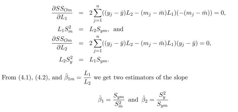
Differentiation of SSOm w.r.t. L1,and L2 and setting them equal to zero, we get
∂SSOm
∂L1
= 2
n ∑
j=1
((yj−y)L¯ 2−(mj−m)L¯ 1)(−(mj −m)) = 0,¯
L1Sm2 = L2Sym, and (4.2)
∂SSOm
∂L2
= 2
n ∑
j=1
((yj−y)L¯ 2−(mj−m)L¯ 1)(yj−y) = 0,¯
L2Sy2 = L1Sym. (4.3)
From (4.1), (4.2), and ˆβ1m=
L1
L2
we get two estimators of the slope
ˆ
β1 =
Sym
S2
m
and ˆβ2 =
Sy2
Sym
(4.4)
Then the geometric mean of the estimators in (4.4) is the GM estimator, that is,
ˆ
β1G=sgn{Sym}
√
S2
y
S2
m
.
Obviously, the above GM estimator is derived by minimizing the orthogonal distance between the
observed point (mj, yj) and unfitted line. Therefore, it does not minimize the distance between the
5
Proposed weighted geometric mean estimator
The proposed weighted geometric mean (WG) estimator minimizes the orthogonal distance between
the observed point (mj, yj) and the unfitted regression line. This estimator is based on the
relation-ship (3.13) between the vertical and orthogonal distances of the observed points and the unfitted
regression line. The WG estimator is derived from equations (4.3) and (4.4).
Multiply equation (4.2) by Sy2,and equation (4.3) bySym,we get
L1Sm2Sy2 = L2SymSy2 (5.1)
L1Sym2 = L2SymSy2, (5.2)
from equation (5.1) plus equation (5.2) we get
L1(Sm2Sy2+Sym2 ) = L22SymSy2
(Sm2Sy2+Sym2 )sinθˆ = 2SymSy2cosθ.ˆ
Hence the proposed estimator which considered it as a weighted geometric mean (WG) estimator is
given by
ˆ
β1W G=
sinθˆ
cosθˆ=
2SymSy2
S2
ySm2 +Sym2
. (5.3)
This estimator could be simplified as follow
ˆ
β1W G =
2Sy2Sm−2
S2
ySym−1+SymSm−2
= 2 ˆβ
2 1G
( ˆβ1+ ˆβ2)
=W βˆ1G, (5.4)
where W = βˆ1G
ˆ
βOLS−mean
, βˆOLS−mean is obtained by taking the arithmetic mean of the slopes of
the two ordinary least squares regression lines of OLS(y/m) and OLS(m/y). Note if the geometric
mean estimator (GME) is equal to OLS-mean estimator, then the proposed weighted geometric mean
estimator (WGE) is equal to both the geometric mean and OLS-mean estimators, becauseW is equal
to one.
The reasons for suggesting weighted geometric mean estimator (WGE) instead of the geometric
mean estimator, and OLS-bisector estimator will be apparent from the results of the next section.
6
Simulation studies
In this section we compare the proposed WG estimator with the GM and OLS-bisector estimators
0 20 40 60 80 100 120 0 1 2 3 4 5 6 7
Ratio of error variances
M e a n s lo p e o f e s ti m a to rs o f tr u e s lo p e = 0 .5 5
(a) Mean slope of estimators and ratio of error variances.
0 20 40 60 80 100 120
0 1 2 3 4 5 6 7
(b) Mean absolute error of estimators and ratio of error variances .
Ratio of error variances
M e a n a b s o lu te e rr o r o f e s ti m a to rs GM OLS-b WG GM OLS-b WG
Figure 2: Graph of the mean slope of estimators, and the mean absolute error when the parameters
β0 = 20, β1 = 0.55 and 0.08≤λ≤100.
We perform large scale simulations to illustrate that the proposed estimator is asymptotically
unbiased and consistent compared to the geometric mean estimator, and OLS-bisector estimator.
The latter estimator is given by
ˆ
β1OLS−B = ( ˆβ1+ ˆβ2)−1 [
ˆ
β1βˆ2−1 +
√
(1 + ˆβ2
1)(1 + ˆβ22) ]
,
where ˆβ1=
Sym
S2
m
,and ˆβ2 =
S2
y
Smy
.
For the simulation, the data set is generated based on 1000 replications of samples size 100 of
normal structural model as follows:
1. Generate 100 independent values x1, . . . , x100 of x∼ N(0,8).
2. Generate 100 independent values u1, . . . , u100 of u∼ N(0,7).
3. Generate 100 independent valuese1, . . . , e100ofe∼N(0, σe),where 2≤σe≤71,for each 1000
replications it is increased by 1.
4. Specify the values ofβ0 and β1 for the regression line.
5. Calculate the values of the three estimators and their mean absolute errors.
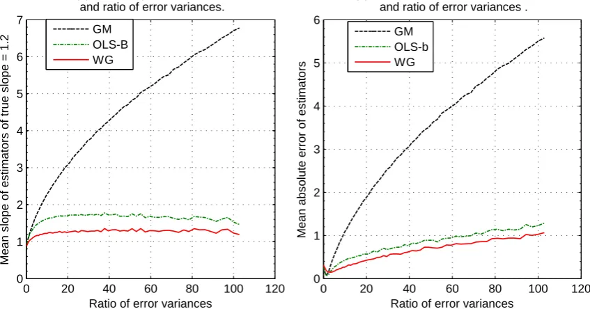
From Figures 1a-3a and under 0.08≤λ≤100,the values of the OLS-bisector estimator are away
from the true values of β1, but it is much closer than those of the geometric mean estimator. The
values of the geometric mean estimator (GME) are far above the true value ofβ1.The GME appears
0 50 100 150 -7 -6 -5 -4 -3 -2 -1 0
Ratio of error variances
M e a n s lo p e o f e s ti m a to rs o f tr u e s lo p e = 0 .7 5
(a) Mean slope of estimators and ratio of error variances.
0 50 100 150
0 1 2 3 4 5 6 7
Ratio of error variances
M e a n a b s o lu te e rr o r o f e s ti m a to rs
(b) Mean absolute error of estimators and ratio of error variances .
[image:13.595.143.567.41.263.2]GM OLS-B WG GM OLS-b WG
Figure 3: Graph of the mean slope of estimators, and the mean absolute error when the parameters
β0 = 27, β1 =−0.75 and 0.08≤λ≤100.
0 20 40 60 80 100 120
0 1 2 3 4 5 6 7
Ratio of error variances
M e a n s lo p e o f e s ti m a to rs o f tr u e s lo p e = 1 .2
(a) Mean slope of estimators and ratio of error variances.
0 20 40 60 80 100 120
0 1 2 3 4 5 6
Ratio of error variances
M e a n a b s o lu te e rr o r o f e s ti m a to rs
(b) Mean absolute error of estimators and ratio of error variances .
GM OLS-B WG GM OLS-b WG
Figure 4: Graph of the mean slope of estimators, and the mean absolute error when the parameters
Table 1: Simulated mean values of the estimated slope and the mean absolute error for various
selected values of the true intercept and slope when 0.08≤λ≤100.
True slope GM OLS-B WG True model
0.55 3.4981 0.9340 0.5904 ηj = 20 + 0.55xj
(MAE) (2.9527) (0.9989) (0.5341)
−0.75 −3.5299 −1.1455 −0.7857 ηj = 27−0.75xj
(MAE) (2.7910) (0.8780) (0.5328)
1.2 3.6321 1.5622 1.2213 ηj =−15 + 1.2xj
(MAE) (2.4676) (0.6548) (0.5302)
0 200 400 600
0 0.5 1 1.5 2
Sample size n
M
e
a
n
s
lo
p
e
o
f
e
s
ti
m
a
to
rs
o
f
tr
u
e
s
lo
p
e
=
0
.5
(a) Mean slope of estimators and ratio of error variances.
GM OLS-b WR
0 200 400 600
0 0.5 1 1.5 2
Sample size n
M
e
a
n
a
b
s
o
lu
te
e
rr
o
r
o
f
e
s
ti
m
a
to
rs
(b) Mean absolute error of estimators and ratio of error variances.
[image:14.595.154.466.185.332.2]GM OLS-b WR
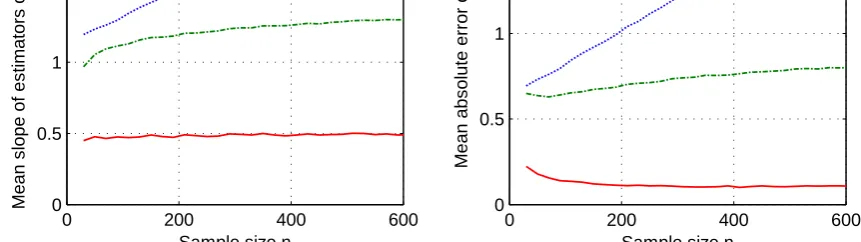
Figure 5: Graph of consistency evaluation of the mean slope of estimators, and the mean absolute
0 200 400 600 800 1000 1200 0.5 1 1.5 2 2.5 3 3.5 4
Sample size n
M e a n s lo p e o f e s ti m a to rs o f tr u e s lo p e = 1
(a) Mean slope of estimators and ratio of error variances.
GM OLS-b WR
0 200 400 600 800 1000 1200 0 0.5 1 1.5 2 2.5 3
Sample size n
M e a n a b s o lu te e rr o r o f e s ti m a to rs
(b) Mean absolute error of estimators and ratio of error variances.
GM OLS-b WR
Figure 6: Graph of consistency evaluation of the mean slope of estimators, and the mean absolute
error when the true β1 = 1 and largeλ.
WGE is much closer to the true values of β1 than other two estimators. It is clear, from Figures
1b-3b that the measurement error makes the mean absolute error of the geometric mean estimator
the highest. While the mean absolute error of the OLS-bisector estimator appears to be smaller
than those of the geometric mean estimator, they are not small. Obviously, the mean absolute
error of the WGE is better and the smallest compared to the other estimators, and it seems to be
stable over the range of selected ratio of error variances 0.08 ≤ λ ≤ 100. Table 1 summarizes the
results of the simulation studies which indicate that the proposed estimator is more precise than the
other competing estimators. Sarach and Celik (2011) discussed eight different regression techniques,
and pointed out that the OLS-bisector estimator is near to the real value than all other regression
techniques, and the mean squares error of OLS-bisector is smaller than all other techniques. The
current study reveals that the proposed WGE is consistently better than the OLS-bisector estimator
in term of the closeness of ˆβ1W G toβ1,and the mean absolute error as shown in Figures 5 and 6.
7
Concluding Remarks
This paper proposes a new estimator based on the mathematical relationship between the vertical and
orthogonal distances of the observed points and the regression line. This estimator is appropriate
to fitting a straight line when both variables are subject to measurement errors, especially when
there is no basis for distinguishing between response and explanatory variables. This method is
Extensive simulation studies confirm that the values of the proposed WG estimator are always
nearer to the true value of the slope more than the OLS-bisector, and the mean absolute error
of WGE is consistently smaller than that of the OLS-bisector. Therefore, the proposed estimator
possesses better statistical proprieties than the geometric mean and OLS-bisector estimators. The
new method is stable and works well for different sample sizes and for different values ofλ.
References
Adcock, R J (1877). Note on the method of least squares. Analyst., 4, 183-184.
Barker, F., Soh, Y C. and Evans, R J. (1988). Properties of the geometric mean functional
relation-ship, Biometrics, 44(1), 279281.
Bartlett, M S. (1949). Fitting a stright line when both variables are subject to error. Biometrics 5,
207-212.
Burr, D. (1988). On Errors-in-Variables in Binary Regression-Berkson Case. J. Am. Statist. Assoc
83, 739-743.
Cheng, C L, and Ness, J W. (1999). Kendall’s Library Of Statistics 6, Statistical Regression With
Measurement Error. New York: Wiley.
Cragg, J G. (1997). Using higher moments to estimate the simple errors-in-variables model. The
RAND Journal of Economics 28, 71-91.
Dent B M. (1935). On observation of points connected by a linear relation. Proc. Physical Soc.
London, 47, 92-108.
Draper, N R. and Yang, Y. (1997). Generalization of the geometric mean functional relationship.
Computational Statistics and Data Analysis 23 355-372.
Durbin, J. (1954). Errors-in-variables. Int. Statist. Rev 22, 23-32.
Feigelson E D, Babu G J. (1992). Linear regression in astronomy. II. Astrophys J 397, 5562.
Freedman, L S, Fainberg, V, Kipnis, V, Midthune, D, and Caroll, R J. (2004). A New Method for
Dealing with Measurement Error in Explanatory Variable of Regression Models. Biometrics 60,
172-181.
Fuller, W A. (2006). Measurement Error Models. New Jersey: Wiley.
Geary, R C. (1942). Inherent relations between random variables. Proc. R. Irish Acad. Sect. A 47,
36-67.
Geary, R C. (1943). Relations between statistics: The general and the sampling problem when the
samples are large. Proceedings of the Royal Irish Academy 49, 177-196.
Geary, R C. (1948). Studies in relations between economics time series. Journal of the Royal
Statistical Society, 10,158-172.
Geary, R C. (1949). Determination of linear relations between systematic parts of variables with
errors of observation the variances of which are unknown. Econometrica 17, 30-58.
Halfon, E. (1085). Regression method in ecotoxicology: a better formulation using the geometric
Halperin, M. (1961). Fitting of straight lines and prediction when both variables are subject to error.
Jou. Amer. Statist. Assoc 56, 657-669.
Isobe T, Feigelson ED, Akritas MG, Babu GJ. (1990). Linear regression in astronomy I. Astrophys.
J. 364, 10413.
Johnson, J. (1972). Econometric Methods. New York: McGraw Hill Book Company.
Jolicouer, P. (1975). Linear regressions in fishery research: some comments. J. Fish. Res. Board
Can. 32(8), 14911494.
Kermack KA, Haldane JBS. (1950). Organic correlation and allometry. Biometrika 37, 3041.
Leng L, T. Zhang, L Kleinman, and W. Zhu (2007). Ordinary least square regression, orthogonal
regression, geometric mean regression and their applications in aerosol science. Journal of Physics
Conference Series 78 012084-012088.
Levinton JS, Allen BJ. (2005). The paradox of the weakening combatant: trade-off between closing
force and gripping speed in a sexually selected combat structure. Funct Ecol 19, 159165.
Ludbrook, J. (2010). Linear regression analysis for comparing two measurers or methods of
mea-surement: But which regression?. Clinical and Experimental Pharmacology and Physiology 37,
692699.
Macdonald J R, Thompson W J. (1992). Least-squares fitting when both variables contain errors:
pitfalls and possibilities. Am J Physiol 60:6673.
Madansky, A. (1959). The fitting of straight lines when both variables are subject to error. Jou.
Amer. Statist. Assoc 54, 173-205.
Maddala, G.S. (2001). Introduction to Econometrics. Prentice Hall International, Inc, Second
edi-tion.
Pal, M. (1980). Consistent moment estimators of regression coecients in the presence of errors in
variables. J. Econometrics 14, 349-364.
Reiersøl, O. (1950). Identifiability of a linear relation between variables which are subject to error.
Econometrica 18, 375-89.
Ricker W. E. (1973). Linear regressions in Fishery research. J Fish. Res. Board Can 30, 409-434
Riggs, D S, Guarnieri, J A and Addelman, S. (1978). Fitting straight line when both variables are
subject to error. Life Sci 22, 1305-1360.
Saqr, A. and Khan, S. (2011) Instrumental variable estimator of the slope parameter when the
explanatory variable is subject to measurement error. In: 11th Islamic Countries Conference on
Statistical Sciences (ICCSS-11), 19-22 Dec 2011, Lahore, Pakistan, pp. 39-53.
Saqr, A. and Khan, S. (2012) Reflection method of estimation for measurement error models. Journal
of Applied Probability and Statistics, 7 (2). pp. 71-88. ISSN 1930-6792
Saqr, A. and Khan, S. (2012a) Slope estimator for the linear error-in-variables model. In: 12th
Islamic Countries Conference on Statistical Sciences (ICCS 2012): Statistics for Everyone and
Saqr, A. and Khan, S. (2016) Mathematical reflection approach to instrumental variable estimation
method for simple regression model. Pakistan Journal of Statistics, 32 (1). pp. 37-48. ISSN
1012-9367
Sladek V, Berner M and Sailer R. (2006). Mobility in central european late neolithic and early bronze
age: femoral cross-sectional geometry. Am J Phys Anthropol 130, 320332.
Sarach S and Celik H (2011). Performance of OLS-bisector regression in method comparison studies.
World Applied Sciences Journal 12(10):1860-1865.
Smith, R J. (2009). Use and Misuse of the Reduced Major Axis for Line-Fitting. American Journal
Of Physical Anthropology 140, 476486.
Sprent, P and Dolby, G R. (1980). Query: the geometric mean functional relationship. Biometrics
36(3), 547-550
Teissier, G. (1948). La relation d’allometrie sa signification statistique et biologique. Biometrics 4,
14-53.
Vaisman, I. (1997). Analytical Geormetry. Singapore: World Scientific.
van Montfort, K. (1989). Estimating in Structural Models with Non-Normal Distributed Varibles:
Some Alternative Approaches. Leiden. DSWO Press.
van Montfort, K., Mooijaart, A., and de Leeuw, J. (1987). Regression with errors in variables:
estimators based on third order moments. Statist Neerlandica 41, 223-237.
Vincent SE, and Lailvaux SP. (2006). Female morphology, web design, and the potential for multiple
mating in Nephila clavipes: do fat-bottomed girls make the spider world go round? Biol J Linn
Soc 87, 95102.
Wald, A. (1940). Fitting of straight lines if both variables are subject to error. Ann. Math. Statist
11, 284-300.
Warton, D I and Wright I J, Falster D S, Westoby M. (2006). Bivariate line-fitting methods for
allometry. Biol Rev 81, 259291.
Willmott, J., and Matsuura, K. (2005). Advantages of the mean absolute error (MAE) over the
root mean square error (RMSE) in assessing average model performance. Climate research, 30(1),
79-82.
Zimmerman F, Breitenmoser-Wu rsten C, Breitenmoser U. (2005). Natal dispersal of Eurasian lynx