STOCHASTIC SYSTEM DESIGN AND APPLICATIONS TO STOCHASTICALLY ROBUST STRUCTURAL CONTROL
Thesis by Alexandros Taflanidis
In Partial Fulfillment of the Requirements for the degree of
Doctor of Philosophy
CALIFORNIA INSTITUTE OF TECHNOLOGY
Pasadena, California 2007
© 2007
Acknowledgements
I would like to firstly thank my advisor, James Beck, for his tireless mentoring throughout my stay at Caltech on both my research and my work as a teaching assistant. He has taught me to be a thorough scientist and a good instructor. I am extremely appreciative of his unwavering support and the amount of freedom he granted me for pursuing my own ideas. I hope we can continue our collaboration for many years to come.
Special thanks go to my good friend Jeff Scruggs for sharing his wisdom with me so patiently in my first two years at Caltech. His guidance has helped me tremendously in getting a better appreciation of the special needs of the structural control field. Similarly many thanks to my good friend and colleague Joseph (Sai-Hung) Cheung for his help on understanding stochastic simulation techniques and the time he always willingly offered for our research-related discussions.
Special gratitude goes to my ex-professors and advisors on my bachelor and Master Thesis, Demos Angelides and Georgios Manos, for their mentoring during those years and their support in my decision to pursue a Ph.D at Caltech. Additional thanks go to Professor Angelides for our close collaboration over the last few years in various research projects.
I have made a lot of good friends at Caltech and I would like to thank all of them for their support. Special thanks go to the famous lunch group: Nick Hudson, Michael Wolf, Moh El Naggar, Joseph Klamo, Kristo Kiecherbaum, Tim Chung, Sam Taira, Judith Mitrani, and of course to Ernie. You guys have made the long hours of graduate school pass quickly. I would also like to thank the SOPS soccer team for entrusting me with the captain position over the last couple of years and sharing with me many happy moments on the soccer field. Special thanks go to Sarah for sharing the last couple of years with me and providing support whenever I needed it.
Last but not least I would like to thank my family, especially my mother, for their unconditional love and support throughout the years.
Abstract
The knowledge about a planned system in engineering design applications is never complete. Often, a probabilistic quantification of the uncertainty arising from this missing information is warranted in order to efficiently incorporate our partial knowledge about the system and its environment into their respective models. In this framework, the design objective is typically related to the expected value of a system performance measure, such as reliability or expected life-cycle cost. This system design process is called stochastic system design and the associated design optimization problem stochastic optimization. In this thesis general stochastic system design problems are discussed. Application of this design approach to the specific field of structural control is considered for developing a robust-to-uncertainties nonlinear controller synthesis methodology.
high plausibility of containing the optimal design variables. An efficient two-stage framework for the stochastic optimization is then discussed combining SSO with some other stochastic search algorithm. Topics related to the combination of the two different stages for overall enhanced efficiency of the optimization process are discussed.
Contents
Acknowledgements iii Abstract v Contents vii
List of Figures xiii
List of Tables xvii
1 Introduction 1
1.1 Stochastic System Design 1
1.2 Structural Control 5
1.2.1 Types of structural control systems 5
1.2.2 Controller design 8
1.3 Overview of the Thesis 10
2 Stochastic System Design: Theoretical Discussion 13
2.1 General Problem 13
2.1.1 Stochastic system model 13
2.1.2 Optimal stochastic system design 16
2.1.3 Stochastic optimization 18
2.3 Controlled System Design 24
2.4 Probabilistic Seismic Ground Motion Model 26
2.4.1 High-frequency component 26
2.4.2 Low-frequency component 29
2.4.3 Model of near-fault ground motions 32
Appendix 2Α: Characteristics of Amplitude Spectrum and Envelope Function for
the Stochastic Method 35
3 Stochastic System Design: Linear Controlled Systems 38
3.1 Linear Time Invariant System Model 39
3.2 Estimation of Stochastic Integrals and Stochastic Optimization for Simple
System Models 42
3.2.1 Asymptotic approximation 43
3.2.2 Stochastic simulation 44
3.2.3 Stochastic optimization 45
3.3 Reliability Calculation for Linear Dynamic Systems 46
3.3.1 Systems with known parameters 47
3.3.2 System including model uncertainty 53
3.3.3 Accuracy and efficiency of the analytical approximation 55
3.4 Nominal Reliability-Based Controller Design 56
3.4.1 Sensitivity of optimal controllers to the out-crossing rate components 57
3.4.2 Optimization considerations 58
3.4.3 Stability of reliability-optimal controllers 60 3.4.4 Relationship to optimal minimum variance controllers 60 3.5 Robust-Reliability Design with Fixed Time Duration 66
3.5.2 Infinite time durations 68 3.6 Robust-Reliability Design with Uncertain Time Durations 69
3.6.1 Short mean time durations 71
3.6.2 Infinite mean time durations 71
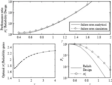
3.6.3 Illustrative example for robust reliability design 72 3.7 Probabilistic Robustness for Minimum Variance Control Design 76
3.7.1 Average robustness for H2 performance 80 3.7.2 Average and reliability robustness for mH2 performance 81
3.8 Concluding Remarks 87
4 Stochastic Subset Optimization 90
4.1 Stochastic Subset Optimization 91
4.1.1 Augmented problem 91
4.1.2 Subset analysis 93
4.1.3 Deterministic subset optimization 96
4.1.4 Stochastic subset optimization 97
4.1.5 Iterative approach 99
4.1.6 Influence of dimension of design variables 100
4.1.7 Sensitivity to the model parameters 101
4.1.8 Details for reliability objective problem 102
4.2 Implementation Issues and Guidelines 103
4.2.1 Characterization and normalization of search space 103
4.2.2 Selection of admissible subsets 106
4.2.3 Identification of the optimal subsets 109
4.2.4 Characteristics for MCMC simulation 110
4.3 Stochastic Subset Optimization Algorithm 113 4.4 Convergence Properties of Stochastic Subset Optimization 117
Appendix 4A: Sampling Techniques 118
Appendix 4B: Relationship between Cartesian and Spherical Coordinates 120 Appendix 4C: Details for Characterization of Admissible Subsets as Hyper-Ellipses 121 4.1C Subset relationship for hyper-ellipses within hyper-cube 122 4.2C Subset relationship for hyper-ellipses within hyper-sphere 123 5 Stochastic System Design: Stochastic Optimization Framework 128
5.1 Stochastic Optimization 128
5.1.1 Common random numbers 128
5.1.2 Exterior sampling approximation 132
5.1.3 Appropriate stochastic optimization algorithms 132 5.1.4 Simultaneous-perturbation stochastic approximation using common
random numbers 134
5.1.5 Objective function approximation methods 136 5.2 Framework for Stochastic Optimization Using Stochastic Simulation 138
5.2.1 Outline of the framework 138
5.2.2 Importance sampling 141
6 Stochastic System Design: Structural Engineering Applications 144 6.1 Optimal Reliability Design of a Base Isolation Protection System 145 6.1.1 Probabilistic system and excitation models 145
6.1.2 Optimization algorithm characteristics 149
6.1.3 Results and discussion for a sample optimization run 151
6.1.5 Accuracy of design identified by SSO 158
6.1.6 Efficiency of stochastic design 159
6.1.7 Sensitivity of design to model prediction error 160 6.1.8 Objective function approximation application 161 6.2 Optimal Life-Cycle Cost-Based Retrofitting of a Four-Story Structure 163
6.2.1 Probabilistic structural model 164
6.2.2 Probabilistic site seismic hazard and ground motion model 166
6.2.3 Expected life-cycle cost 168
6.2.4 Optimal damper design 175
6.2.5 Details for stochastic subset optimization 175 6.2.6 Details for simultaneous-perturbation stochastic approximation with
common random numbers 176
6.2.7 Efficiency of the two-stage optimization framework 178 6.2.8 Efficiency of seismic protection system 179 7 Stochastic System Design: Structural Control Applications 184
7.1 Protection of Base-Isolated ASCE Benchmark Structure 186
7.1.1 Benchmark structure 187
7.1.2 Control implementation details 190
7.1.3 RFA Network 191
7.1.4 Control law selection 192
7.1.5 Controller design 196
7.1.6 Controller design optimization 199
7.1.7 Performance evaluation 201
7.2 Controller Design for Offshore Platforms 212
7.2.1 Model for Tension Leg Platform 214
7.2.3 Control implementation for Tension Leg Platform 220 7.2.4 Equation of motion for controlled system 222
7.2.5 Controller Design 224
7.2.6 Performance evaluation 226
8 Conclusions 232
8.1 Summary and Main Contributions 232
8.1.1 Chapter 2 232
8.1.2 Chapter 3 233
8.1.3 Chapter 4 235
8.1.4 Chapter 5 236
8.1.5 Chapter 6 237
8.1.6 Chapter 7 239
8.1.7 Conclusions 240
8.2 Future Work 240
List of Figures
Figure 1.1: Illustration of (a) electromechanical actuators and (b) RFA
network application (taken from Scruggs et al. 2007a) 7 Figure 2.1: Representation of (a) initial and (b) augmented system model 14 Figure 2.2: Comparison between analytical and simulation-based (sim)
evaluation of an objective function 20
Figure 2.3: Representation of controlled system model 25 Figure 2.4: Radiation spectrum, envelope function, and sample excitation
according to the stochastic ground motion method 28 Figure 2.5: Sample near-fault ground motion: acceleration and velocity time
histories 34 Figure 3.1: Three-dimensional example of failure surfaces 46
Figure 3.2: Spatial correlation between failures of performance variables z1
and z2 51
Figure 3.3: Cases for which the Poisson approximation to out-crossing
times is not a good model 52
Figure 3.4: Structural model 61
Figure 3.5: Comparison between optimal multi-objective H2 and reliability
designs 63 Figure 3.6: Comparison between optimal H2 and reliability designs 65
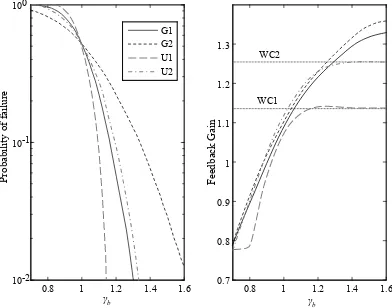
Figure 3.7: (a) Probability of failure under optimal robust-reliability design and (b) normalized optimal gain for UC1(black curves) and
Figure 3.8: Statistics of the out-crossing rate over the uncertain parameter space for optimal robust reliability controller assuming
deterministic time duration T for (a) UC1 and (b) UC2 75 Figure 3.9: Percentile improvement in reliability performance under robust
design compared to the nominal design for UC1(black curves)
and UC2 (grey curves) 76
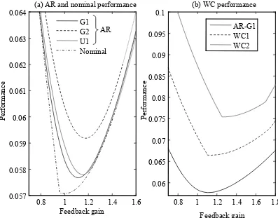
Figure 3.10: Nominal, average, and worst case H2 performance for
variations of the feedback gain 81
Figure 3.11: Nominal, average, and worst case mH2 performance for
variations of the feedback gain 82
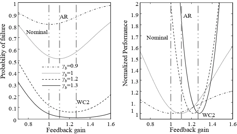
Figure 3.12: (a) Probability of failure under optimal design and (b) corresponding optimal gain for RR design for variation of the acceptable performance threshold. Horizontal lines in plot (b)
correspond to optimal gain for WC design methods 83 Figure 3.13: RR performance for variation of the feedback gain for U1 case
for model uncertainty. Vertical lines correspond to optimal
controller for other synthesis methods 84
Figure 3.14: RR performance for variation of the feedback gain for G1 case for model uncertainty. Vertical lines correspond to optimal
controller for other synthesis methods 84
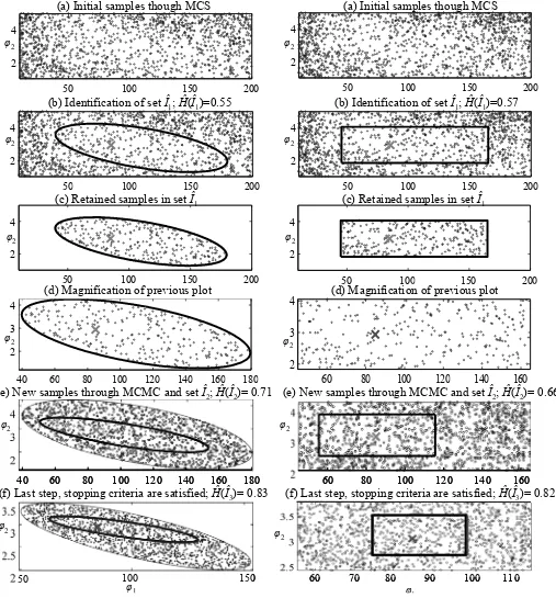
Figure 4.1: Example for the quality of identification for two cases 98
Figure 4.2: Adjustment of initial search space 105
Figure 4.3: Influence of selection of s in SSO 113
Figure 4.4: An illustrative example for the SSO algorithm for selection of admissible subsets as hyper-ellipses (left) or hyper-rectangles
(right) 115 Figure 4.5: Some important steps for the SSO algorithm for selection of
admissible subsets as hyper-ellipses (left) or hyper-rectangles
Figure 5.1: Evaluation of objective function using common random
numbers (CRN) 130
Figure 5.2: Illustration of CRN application in ROP: (a) the two possible performance measures and (b) comparison between the
estimated objective functions using these two choices 131
Figure 6.1: Base-Isolated structure 146
Figure 6.2: Details about importance sampling densities formulation 150
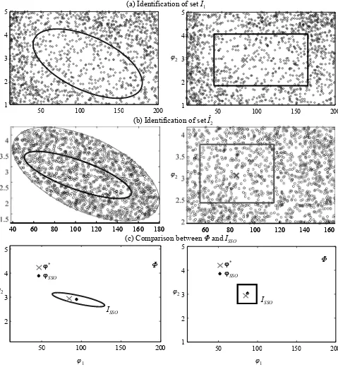
Figure 6.3: Sets ISSO (ellipse) and Φ (rectangle) for problem D1 152 Figure 6.4: Projections of sets ISSO (ellipse) and Φ (rectangle) onto the
planes of all pairs for the design parameters for problem D2 153 Figure 6.5: Optimal design variables and performance for various instances
of the model prediction error for design problem D1 160
Figure 6.6: Illustration of OAM application for design problem D1 162
Figure 6.7: Structural model assumed in the study 164
Figure 6.8: (a) Mean occurrence rate, and probability of occurrence for (b) tdur=1 year and (c) tdur=60 years, for PGA (peak ground
acceleration) and PSA ( peak spectral acceleration) 168 Figure 6.9: (a) Fragility functions for structural components and (b)
restoring force-drift relationship 171
Figure 6.10: (a) Fragility function and (b) damage state probabilities for
partitions 173 Figure 6.11: Total expected repair cost for the (a) drift and (b) acceleration
sensitive components (per story) 173
Figure 6.12: Expected repair cost for the drift sensitive damageable
assemblies (per story) 174
Figure 6.13: Details about importance sampling densities formulation 178 Figure 6.14: Details about expected life-cycle cost 180 Figure 6.15: Distribution of repair and life-cycle cost between different
Figure 6.16: Distribution of repair, damper and life-cycle cost between different stories. Maximum force capacity of the dampers for
each story is also illustrated 183
Figure 7.1: (a) Base plan of the benchmark structure and (b) side view 189 Figure 7.2: Feasible force region for regenerative and semi-active two
actuator system 191
Figure 7.3: Seismological model for the site of the structure and resultant
probability models 198
Figure 7.4: Block diagram of simulated controlled system at design stage 200 Figure 7.5: Time-histories for recorded earthquake records used in this
study 203 Figure 7.6: Scatter plots of threshold-normalized response for the four
groups of performance variables for the 14 ground motion cases 206 Figure 7.7: Base displacement at southeast corner for (a) Sylmar and (b) Jiji
earthquakes acting in FP-y direction 210
Figure 7.8: Displacement-force plot for the friction pendulum isolator at southeast corner for (a) uncontrolled and (b) RFA equipped
structure for the Sylmar earthquake acting in FP-y direction 211 Figure 7.9: Desired and feasible resultant forces at the center of mass of the
base for the Sylmar earthquake acting in FP-y direction 212 Figure 7.10: Tension Leg Platform with degrees of freedom 215 Figure 7.11: Tension Leg Platform model considered in the study 216 Figure 7.12: Schematic of passive and active TMD implementation 221 Figure 7.13: (a) PM spectrum and eigenfrequencies of TLP (arrows) and (b)
a sample realization of η(t) 224
Figure 7.14: Sample time histories for heave displacement and tendon stress
for simulated sea state with properties Hs=9 m, Tz=10.6 sec 228
List of Tables
Table 2.1 Parameters for predictive relationships for near-fault pulse
characteristics 31 Table 6.1 Results from a sample run of the SSO algorithm for two design
problems 152 Table 6.2 Cumulative results from a sample run of the optimization
framework 152 Table 6.3 Efficiency for identification of optimal design using SSO only 158
Table 6.4 Characteristics of fragility functions and expected repair cost for
each story 170
Table 6.5 Relationship between damage states for “structural components” damageable assembly and type of repair needed for the beams
and columns 172
Table 6.6 Optimization results 175
Table 7.1 Periods and participation factors for superstructure 188 Table 7.2 Reliability-related statistics for various controller designs 201 Table 7.3 Performance evaluation criteria for recorded excitations; FX-x
case 204 Table 7.4 Performance evaluation criteria for recorded excitations; FP-y
case 204
Table 7.5 Details of TLP 223
CHAPTER 1
Introduction
1.1
Stochastic System Design
In engineering design, the knowledge about a planned system is never complete. First, it is not known in advance which design will lead to the best system performance in terms of a specified metric; it is therefore desirable to optimize the performance measure over the space of design variables that define the set of acceptable designs. Second, modeling uncertainty arises because no mathematical model can capture perfectly the behavior of a real system and its environment. In practice, the designer chooses a model that he or she feels will adequately represent the behavior of the built system as well as its future excitation; however, there is always uncertainty about which values of the model parameters will give the best representation of the constructed system and its environment, so this parameter uncertainty should be quantified. Furthermore, whatever model is chosen, there will always be an uncertain prediction error between the model and system responses. For an efficient engineering design, all these uncertainties, associated with future excitation events, as well as the modeling of the system, must be explicitly accounted for.
different properties of the system by a probability model which is implicitly conditioned on available knowledge. The specific probability model chosen represents the expected information gain based on the knowledge we have about the system; this gain is quantified in terms of the absolute or relative information entropy (Shannon 1948; Papadimitriou et al. 2000). In this context, choosing a probability model with the largest entropy is equivalent to incorporating the largest possible uncertainty into the system description, subject to the available information. For example, subject to specifications of the first and second moments (or, equivalently, expected value and variance) for a continuous variable that is restricted within some range, the most appropriate, in the aforementioned context, probability model selection is a truncated Gaussian probability density function; if no specification is made of the moments of the variable, then the most appropriate selection is a uniform probability density function. This knowledge-based interpretation of probability leads to a logical consideration of all system uncertainties without requiring the introduction of the non-rigorous concept of “inherent randomness” and, ultimately, to a powerful framework for formulating the design problem and performing the required optimization. In this work, this design process is called stochastic system design.
It should be noted that even though the theoretical ideas for design considering modeling uncertainties were introduced many decades ago, the computational cost associated with this design methodology—because of the complex coupling between system modeling, stochastic analysis, and optimization—has reduced the range of applications considered. Often the formulation of stochastic design problems is restricted by the available computational resources and the ability to perform the associated design optimization. For complex systems this has often dictated (a) use of mathematical models that do not adequately consider all characteristics of the true system behavior, or (b) adaptation of approximate techniques for evaluating their performance in a probabilistic setting. Recent advances in software and hardware computer technology have contributed to overcoming many of these restrictions and the general concept of stochastic system design is rapidly spreading to new types of applications.
In RBDO a particular source of difficulty is the high computational cost associated with a single reliability analysis. Even though relatively efficient algorithms have been recently developed for calculation of failure probabilities for complex systems (Au and Beck 2001a; Au and Beck 2001b; Schueller et al. 2004), each evaluation still requires a substantial computational effort, particularly for dynamic reliability problems. To reduce this computational effort, many specialized approaches have been proposed for reliability-based optimizations. These approaches include, for example, use of some proxy for the failure probability (e.g., reliability index obtained through first-order or second-order analysis, as, for example, in Enevoldsen and Sorensen (1994)), and response surface approximations to the limit state function defining the model’s response for each design choice (e.g., Gasser and Schueller (1997)). Such specialized approaches may work satisfactorily under certain conditions, but are not proved to converge to the solution of the original design problem. This is particularly true for optimization problems that involve the reliability of the system as the objective function, rather than as constraint as commonly adopted in RBDO, because the sensitivity of the objective function to some design variables can be highly complex and not accurately described through approximate techniques.
Special attention is given to design problems involving structural control applications. Therefore, before outlining in more detail the goals and the plan of the thesis, the general characteristics of structural control design are briefly discussed.
1.2
Structural Control
Over the last three decades, there has been a growing interest in the application of control technologies for civil structures in order to reduce their dynamic response and to increase the system reliability with respect to future dynamic excitations, e.g., wind, earthquakes, sea waves. The extensive efforts of many researchers have yielded numerous manifestations of this idea, resulting in several distinct actuation strategies and controller designs. Several state-of-the-art reports (Housner et al. 1997; Spencer and Nagarajaiah 2003; Dyke 2005) provide a detailed survey.
1.2.1
Types of structural control systems
The most fundamental distinction between the different control systems in civil engineering is based on their energy requirements. The three major classes may be defined as follows:
Passive systems: do not require an external power source for operation and utilize the motion of the structure to develop dissipative local control forces. They represent, today, the biggest percentage of full-scale structural control implementations and include various types of mechanical devices, for example, viscoelastic dampers, tuned mass dampers, liquid column mass dampers, and friction dampers.
Semi-active systems: also utilize the motion of the structure to develop dissipative control forces but they use feedback measurements to alter the characteristics of the dissipative mechanism in real time. The external power source requirements are orders of magnitude smaller than active systems or their dissipative capabilities. Different types of semi-active devices have been proposed for civil engineering structures, such as variable orifice dampers, variable friction dampers, variable stiffness devices, and controllable fluid dampers. Most of these devices dissipate energy through mechanical means.
Of these different classes active systems give the greatest improvement of the structural response under dynamic excitations. However, they possess great disadvantages in their significant power requirement, which for large structures are typically too big to be met with local supplies. This raises a question for practicality and also for reliability, since control in civil engineering applications aims at the protection of structures from extreme events (e.g., strong earthquakes, high winds, tidal waves) during which the electrical power grid is susceptible to destabilizations and blackouts. Because of this limitation of active systems, the focus of research has shifted to semi-active ones which have power requirements that can be satisfied by local supplies and at the same time allow, though in a limited range, for real-time force control, making them superior to passive systems (Symans and Constantinou 1999).
addition to providing local dissipation (as do semi-active devices), it is possible for an RFA network to transmit energy between remote locations in a structure. The network, as a whole, must always dissipate energy, which imposes a constraint on the system forcing capabilities and makes the synthesis of control laws challenging. Thus, like semi-active devices, the power required for operation of the electromechanical actuators in the RFA network is only that required for the sensing and intelligent controller systems, which, contrary to the requirements of fully-active systems, can be provided by a small local power supply. This feature makes them appropriate devices for structural control applications. i1 i2 f2 v2 f1 v1 iR1 V1 + − V1 + − V2 + − V2 + − iR2 R1 R2 i1 i2 f2 v2 f1
v1 V1 iR
+ − V1 + − V2 + − V2 + −
dissipative element
i1 i2 f2 v2 f1 v1 iR1 V1 + − V1 + − V2 + − V2 + − iR2
(a) Semi-active actuation
R1 R2 i1 i2 f2 v2 f1
v1 V1 iR
+ − V1 + − V2 + − V2 + −
(b) Regenerative actuation
Vi: voltage
ii: current
Ri: resistance
Figure 1.1: Illustration of (a) electromechanical actuators and (b) RFA network
application (taken from Scruggs et al. 2007a)
can be big, this limitation can be fairly important for the overall quality of the controlled system.
1.2.2
Controller design
In considering the application of advanced actuation technologies for structural control, one fundamental question is whether the versatility afforded by the technology justifies the associated increased cost and maintenance issues, beyond those of simpler passive systems? The answer to this question has as much to do with the feedback control law as it does with the physical limitations of the device’s hardware. A high-quality control system requires that one designs the feedback controller with specific control objectives in mind, related to meaningful structural performance measures, while at the same time addressing actuator and system nonlinearities and the uncertainties in the system and excitation models. Note that because of the physical constraints for the actuators used in typical structural control applications, the usual stability-robustness issues in control system design do not apply to these problems. Thus, the performance of the controlled system is the only metric by which the quality of the control design should be judged.
Most of the research efforts on control law design for structural applications have been on extending linear control methodologies, primarily some variant of H2control, to structural
control techniques. However, they do not lead to controllers which directly optimize meaningful global measures of dynamic structural performance, such as drifts, accelerations, etc. Ad-hoc methods (the popular "clipped-optimal" control for example) that do incorporate such global measures in the controller optimization have also been suggested. Typically, such controllers are designed in an iterative fashion, in which controller performance is qualitatively assessed for successive design iterations through simulation. For structural control applications with few actuators and one dominant mode, this approach is often sufficient to arrive at a satisfactory controller but still cannot, in general, guarantee any bound on the level of performance actually attained (Scruggs et al. 2007a). Recently, a simple controller synthesis methodology has been developed that can guarantee easily-computable upper bounds on the stochastic stationary performance for semi-active and regenerative systems (Scruggs 2007; Scruggs et al. 2007a; Scruggs et al. 2007b) as long as the dynamical system and excitation models are linear. Note that most aforementioned methodologies primarily focus on the mean square structural response and do not explicitly account for uncertainties in the system and excitation models.
probabilistic uncertainty was addressed in Wang and Stengel (2002), and the robust performance in Spencer et al. (1994). Monte Carlo simulation and FORM/SORM, respectively, have been used in these studies for the reliability evaluations but minor attention has been given on the complexity of the associated controller design optimization. The first-passage failure probability has also been used as a reliability performance objective for structural control applications; an approach originally proposed in May and Beck (1998) for systems with probabilistic parameter uncertainty and stochastic excitation, and further elaborated in Yuen and Beck (2003) and Scruggs et al. (2006). An upper bound for the first-passage failure probability has been used as a reliability measure in all these studies, calculated by neglecting the correlation between the different modes of system failure. For linear dynamical systems under stationary excitation that do not include uncertainty for the model parameters, reliability constraints have been applied in performance optimization based on covariance control design in Field and Bergman (1998). Note that all research efforts referenced in this paragraph have been restricted to linear controlled system models.
1.3
Overview of the Thesis
the specific field of structural control are discussed for deriving a robust-to-uncertainties nonlinear controller design methodology. This design approach addresses the challenges discussed earlier related to control law synthesis for structural control applications.
Chapter 2 outlines the stochastic system design problem and discusses the challenges involved in the associated optimization process when stochastic simulation is used for evaluating the model performance. A probabilistic model for characterizing the system excitation in earthquake engineering applications is also developed. This model establishes a direct link between the probabilistic seismic hazard description of the structural site and future ground motions and can efficiently describe both the far-field and the near-field characteristics of the latter.
In Chapter 3 design problems are addressed that involve relatively simple models. Special focus is given on the design of control laws for linear structural systems with probabilistic model uncertainty, under stationary stochastic excitation. The focus is primarily on reliability-based synthesis. An analytical approach, motivated by the simplicity of the models adopted, is discussed for the design problem. This approach gives useful insight into the characteristics of the controller synthesis and allows for direct comparison to other design methods that have been proposed for such applications. An accurate analytical approximation for the first-passage failure probability is presented and questions are addressed related to stability, optimality, relationships to minimum variance synthesis, and appropriate characterization of robust-reliability for control applications in which model uncertainty is included. Τhis chapter also contains an investigation of the influence of probabilistic quantification of model uncertainty on classical control approaches, such as
H2 and multi-objective H2 designs.
presents a novel algorithm, called Stochastic Subset Optimization (SSO), for efficiently exploring the sensitivity of the objective function to the design variables and iteratively identifying a subset of the original design space that has high plausibility of containing the optimal design variables. Statistical properties, appropriate stochastic simulation techniques for complex system models, and stopping criteria for the iterative approach are presented. An efficient two-stage framework for the stochastic optimization is then discussed in Chapter 5 by combining SSO with some other stochastic search algorithm. Topics related to these algorithms, as well as to the combination of the two different stages for overall enhanced efficiency and accuracy of the optimization process, are discussed.
CHAPTER 2
Stochastic System Design: Theoretical Discussion
This chapter outlines initially the stochastic system design problem and presents the challenges involved in the associated optimization process when stochastic simulation is used for evaluating the model performance. The details of reliability-based performance evaluation are then discussed and the implementation of this general methodology to the specific field of structural control is introduced. Since the applications in this thesis focus primarily on earthquake engineering, a probabilistic excitation model for describing earthquake ground motions is also developed here. This stochastic ground motion model can efficiently represent both far-field and near-field characteristics of ground motions. This model has also been published in Taflanidis et al. (2007b).
2.1
General Problem
2.1.1
Stochastic system model
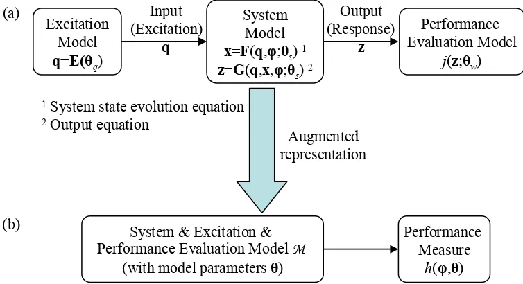
Consider a system that includes some controllable parameters that define the system design, referred to herein as design variables, φ=[φ1,φ2,...,φnφ]∈Φ⊂
φ
n
averaged over the whole set of model classes using probabilistic weighting factors for each one that correspond to its relative plausibility. The model class M in this study represents the augmentation of the individual system, excitation, and performance evaluation models that the designer has chosen, as shown in Figure 2.1. The whole analysis is conditioned on the chosen model class M. For notational simplicity this conditioning is not explicitly noted in the subsequent probability models for the system and its environment. Each model in the class is specified by a nθ-dimensional vector θ=[θ1,θ2,...,θnθ] lying in Θ⊂
nθ
\ , the set of possible values for the model parameters. Because there is uncertainty in which model best represents the system behavior, a PDF (probability density function) p(θ|φ), which incorporates our available prior knowledge about the system and its environment, is assigned to these parameters. The PDF p(θ|φ) should be interpreted as a measure of the relative plausibility of the model defined by θ∈Θ (Jaynes 2003); all probabilistic results are implicitly conditional on the chosen probability model for p(θ|φ).
Excitation Model
q=E(θq)
System Model
x=F(q,φ;θs) 1 z=G(q,x,φ;θs) 2
Input (Excitation)
q
Performance Evaluation Model
j(z;θw) Output
(Response)
z
System & Excitation & Performance Evaluation Model M
(with model parameters θ)
Performance Measure
h(φ,θ) Augmented
representation
1System state evolution equation 2Output equation
(a)
[image:32.612.137.514.387.592.2](b)
Figure 2.1: Representation of (a) initial and (b) augmented system model
supported by this knowledge. Such knowledge may come from observations of similar systems. The principle of maximum information entropy (Jaynes 2003) can be used for quantifying in a logical manner this knowledge. The probability models that are chosen according to this principle express the maximal uncertainty about the values of the model parameters, given all prior information. If any other choice is made there should be strong grounds for the implied reduction in uncertainty in the modeling. Some examples have been discussed in Section 1.1. If data are available from the behavior of the actual system, then the additional information contained in them can be used to update the probability model p(θ|φ) using a Bayesian statistical framework (Beck and Katafygiotis 1998; Beck and Au 2002; Muto and Beck 2007). In the case that more than one model class M is being considered as a candidate for the analytical system model, the information in the data can be also used to update the relative plausibility of the different model classes and possibly perform model class selection (Beck and Yuen 2004; Muto and Beck 2007).
With regard to the excitation model, the uncertainty in the model description may stem from (a) the representation of a sample realization of the system stochastic input, assuming that its characteristics (for example, spectral properties) are known, but additionally from (b) the incomplete knowledge about these characteristics related to anticipated future excitations. Typically, the first type is expressed by using a stochastic sequence, commonly a white-noise sequence, as input to the excitation model, and the second by assigning PDFs to the parameters defining the properties of this model. The uncertain model parameter vector for the excitation model, denoted θq in Figure 2.1, expresses both these sources of
uncertainty.
components that comprise the augmented system model; that is, for those components that, in the modeling context, can be considered as (stochastically) independent. Alternatively, one single prediction error can be considered for the performance of the augmented system that combines the errors that may exist for all individual components. No matter how the influence of the model prediction error is incorporated into the augmented system model, the error itself can be modeled probabilistically as a random variable (Beck and Katafygiotis 1998) and can be augmented into θ to form an uncertain parameter vector, comprised of both the uncertain model parameters and the model prediction error. The selection of the probability model for this error follows the same guidelines as discussed earlier for the other model parameters; the principle of maximum information entropy can be implemented for quantifying the available prior information. In most design problems, knowledge of only the mean value and the expected spread (variance) of the error is typically available. For such cases, the maximum entropy principle indicates that a Gaussian PDF should be selected for probabilistically characterizing the prediction error. In applications for which the errors associated with each independent system-model component are separately considered, the maximum entropy principle indicates that these errors should be modeled as uncorrelated variables.
2.1.2
Optimal stochastic system design
The favorability of different system designs, given the values of the system’s model parameters, is evaluated by the function h(φ,θ):\nφx\nθ →\, which corresponds to the
performance measure of the system response. The convention that lower values of h(φ,θ) correspond to better performance is adopted herein. In the stochastic setting considered, the performance of the system may be expressed in terms of the stochastic integral:
[ ( , )] ( , ) ( | )
Θ
where Eθ[.] denotes expectation with respect to the PDF for θ. Through appropriate
definition of h(φ,θ) this performance objective can correspond to many different interpretations—for example, system reliability, as in (2.8) or (2.12), or expected life-cycle cost, as in (6.15). Equivalently, h(φ,θ) can be considered as a utility function (see, for example, Porter et al. (2004b)) that quantifies the preference for the different outputs of the system (response z in Figure 2.1).
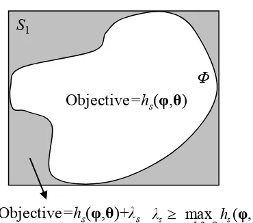
Τhe function in (2.1) corresponds, then, to the objective for a robust-to-uncertainties design. We then have the optimalstochastic system design problem:
minimize [ ( , )] subject to ( ) 0c
E h
≥
θ φ θ
f φ (2.2)
where fc(φ) corresponds to a vector of constraints, which can be either deterministic or
correspond to stochastic integrals (like the objective function). Such optimization problems, arising in decision making under uncertainty, are typically referred to as stochastic optimization or stochastic programming problems, e.g., Ruszczynski and Shapiro (2003), Marti (2005). A key difficulty in these problems is in dealing with an uncertainty space that is large and it frequently leads to a challenging evaluation of the multi-dimensional integral in (2.1). Optimization (2.2) may be further complicated by the presence of (i) design constraints that are also expressed as stochastic integrals, or (ii) integer design variables that model logical and other discrete design selections. In the current study the focus is primarily on problems that involve continuous design variables and deterministic constraints. Optimization (2.2) may be then equivalently formulated as the determination of:
arg min [ ( , )]
*
E h
∈
= θ
φ
φ φ θ
Φ
(2.3)
where the deterministic constraints are taken into account by appropriate definition of the admissible design space Φ.
2.1.3
Stochastic optimization
in detail in Chapter 3. For complex systems, though, this is rarely true, and so the objective function can be typically estimated only by stochastic simulation techniques. In this setting, an unbiased estimate of the expected value in (2.1) can be obtained, for example, by direct Monte Carlo integration using a finite number, N, of random samples of θ, drawn from p(θ|φ):
,
1 1
ˆ [ ( ,N N)] N ( , )i
i
E h h
N =
=
∑
θ φ Ω φ θ (2.4)
where ΩN=[θ1 ... θΝ] is the sample set of the model parameters with vector θi denoting the
sample of these parameters used in the ithsimulation. In this stochastic simulation-based setting, the system response can be evaluated through computer simulation, rather than approximated analytically. This allows for efficiently addressing nonlinearities of the system models and complex performance metrics.
The quality of the estimate (2.4) is quantified in terms of its coefficient of variation, denoted as c.o.v., which is defined as the ratio of the standard deviation of the estimate over its mean value and can be expressed by (Fishman 1996):
(
)
22 2 , 1 , ( , ) [ ( , )] 1 c.o.v. [ ( , )] 1 ˆ ( , ) [ ( , )] 1
ˆ [ ( , )]
u
N
i N N
i
N N
E h E h
Δ
E h N N
h E h
N E h N = ⎡ − ⎤ ⎣ ⎦ = = ⎡ − ⎤ ⎣ ⎦ ≈
∑
θ θ θ θ θφ θ φ θ
φ θ
φ θ φ Ω
φ Ω
(2.5)
where Δuis the unit coefficient of variation for the estimator in (2.4).
The estimate of Eθ[h(φ,θ)] in (2.4) involves an unavoidable error eN(φ,ΩΝ) which is a
defined by the design variable selection φ. The optimization in (2.3) is then approximated by:
ˆ
arg min [ ( , )]
*
N E h N
∈
= θ
φ
φ φ Ω
Φ
. (2.6)
If the stochastic simulation procedure is a consistent one, then as N→ ∞, ,
ˆ [ ( ,N N)] [ ( , )]
Eθ h φ Ω →E hθ φ θ and * *
N →
φ φ under mild regularity conditions for the optimization algorithms used (Ruszczynski and Shapiro 2003). The existence of the estimation error eN(φ,ΩΝ), which may be considered as noise in the objective function,
contrasts with classical deterministic optimization where it is assumed that one has perfect information. Optimization (2.6) is also closely related to the general field of simulation-based optimization (see, for example, Gosavi (2003)) since the objective function is obtained by means of a simulation-based approach.
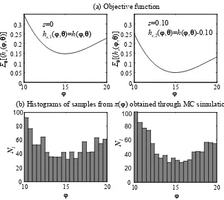
analytical simN =1000 simN =4000
φ Eθ
[(
h
(
φ
,
θ
)]
Figure 2.2: Comparison between analytical and simulation-based (sim) evaluation of an objective function
Figure 2.2 illustrates the difficulties associated with eN(ΩΝ,φ). The curves corresponding to
estimated optimum depends on the exact influence of the estimation error, which is not the same for all evaluations; different runs of the algorithm might converge to different solutions, which do not necessarily correspond to the true optimum. Another source of difficulty, especially when complex system models are considered, is the high computational cost associated with the estimation in (2.4), since N system analyses must be performed for each objective function evaluation. Even though recent advanced stochastic optimization algorithms (see Chapter 5) can efficiently address the first two aforementioned problems, this latter one remains challenging for many engineering design applications. Specialized, approximate approaches have been proposed in various engineering fields for reduction of the computational cost (for example, for reliability-based optimal design problems as discussed earlier in Section 1.1). These approaches may work satisfactorily for certain applications, but typically cannot be proved to converge to the solution of the original design problem. For this reason such approaches are avoided in this current study. Optimization problem (2.6) is directly solved so that * *
N ≈
φ φ .
2.2
Reliability-Based Design
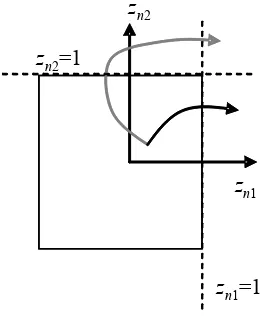
The reliability of the system reflects the plausibility of occurrence of unacceptable performance, based on all available information. Let z∈\nz correspond to the system response vector, Ds be the region in z space that defines the acceptable system performance
and g(φ,θ) be the limit state function that defines the system unacceptable performance, referred to as failure, with the convention that g(φ,θ)≥0 denotes the failure region in the θ space. Note that the failure region can be determined either in terms of the response vector space or the model parameter vector θ, since the latter includes the performance evaluation and system input model parameters. The reliability of the system for specified design variables φ is quantified by the failure probability:
(
)
(
)
( | ) ( , ) 0
F s
P φ Θ =P z∉D =P g φ θ ≥ (2.7)
where P denotes probability. System model uncertainties can be taken into account in this formulation by employing the idea of robust probability of failure (Papadimitriou et al. 2001). This probability is expressed as:
( , ) 0
( | ) [ ( , )] ( , ) ( | ) ( | ) ( | )
f
F F Θ F
g Θ
P Θ E I I p d
p d p d
≥
= =
= =
∫
∫
∫
θ
φ θ
φ φ θ φ θ θ φ θ
θ φ θ θ φ θ (2.8)
where ΙF(φ,θ) is the indicator function of failure, which is 1 if the system model that
corresponds to (φ,θ) fails, i.e., its response departs from the acceptable performance set, and 0 if it does not, and Θf is the region in the Θ space that leads to unacceptable
If direct Monte Carlo estimation is used for evaluation of the integral in (2.8) the c.o.v. in (2.5) may be further simplified to (Au and Beck 2001a):
ˆ
1 ( | )
c.o.v.
ˆ ( | )FF
P Θ
N P Θ
− ≈
⋅
φ
φ . (2.9)
An equivalent expression can also be derived for the robust failure probability by explicitly considering the influence of the model prediction error between the responses of the actual system and the assumed model. Let g( , )φ θ be the limit state function defining the model’s failure, and let the model prediction error, ε(φ,θ), be defined in such a way that the relationship
( , ) g( , ) g( , )
ε φ θ = φ θ − φ θ (2.10)
holds. In this context, and noting that g(φ,θ)>0 corresponds to g( , )φ θ >ε( , )φ θ , PF(φ|Θ) is
transformed into:
( , ) 0 ( , ) ( , )
( | ) ( , , ) ( | ) ( ) ( | ) ( )
= ( | ) ( ) ( | ) ( )
F Θ F g
g
Θ g Θ
P Θ I p p d d p p d d
p p d d p p d d
ε
ε ε ε ε ε
ε ε ε ε
∞ −∞ > > −∞ = = ⎡ ⎤ = ⎢ ⎥ ⎣ ⎦
∫ ∫
∫ ∫
∫ ∫
∫
∫
φ θ φ θ φ θφ φ θ θ φ θ θ φ θ
θ φ θ θ φ θ
(2.11)
where in this case the vector θ corresponds solely to the uncertain parameters for the system and excitation model, i.e., excluding the model prediction error. The last integral (in brackets) in (2.11) can be analytically solved: it corresponds to ( ( , ))P gε φ θ , where Pε is
the cumulative distribution function for the model prediction error ε conditioned on (φ,θ). The robust failure probability in (2.8) is then expressed by
( | ) [ ( ( , ))] ( ( , )) ( | )
F Θ
Thus, the performance measure in optimal reliability problems corresponds either to (a) h(φ,θ)=ΙF(φ,θ) or (b) h(φ,θ)= ( ( , ))P gε φ θ , depending on which formulation is adopted,
(2.8) or (2.12). The optimal reliability problem is formulated as
arg min ( | )
*
F
P Θ
∈
=
φ
φ φ
Φ
. (2.13)
Note that expressions similar to (2.12) may de developed by considering different characterizations for the influence of the model prediction error, for example, by taking it into account directly with respect to the model response, z, as in Papadimitriou et al. (2001). Typically there is some form of equivalence between these different characterizations. For example, the definition of the limit state function along with relationship (2.10) leads automatically to a specific relationship between the assumed model and the actual system responses. Special care is needed so that the first definition leads to a realistic relationship in the latter case, in the context of the specific application and the probabilistic model considered for the prediction error.
2.3
Controlled System Design
This system can be easily represented in the augmented form of Figure 2.1. Thus the general stochastic system design formulation discussed earlier can be naturally extended to control applications to develop a robust-to-uncertainties nonlinear controller design methodology. The simulation-based methodology discussed earlier will contribute to explicit consideration of all important, linear or nonlinear, characteristics of the system model at the design stage, but will lead to a challenging controller optimization problem, especially for systems that include higher-order controllers with large dimensional parameter vectors. For controlled systems it is interesting to compare how the stochastic design approach compares to classical methodologies that have become the standard tools for controller synthesis. Some insight to this question will be given in Chapter 3. Because of their greater familiarity in the control literature, Chapter 3 will address the design of control laws for linear structural systems with probabilistic model uncertainty, under stationary stochastic excitation. An analytical approach, motivated by the simplicity of the models, will be discussed for this design problem that gives useful insight in the characteristics of the controller synthesis and allows for direct comparison to other controller design methods that have been proposed for such applications.
Desired Control Force
ud
Excitation Model System Model Outputz
Sensor Model
Control Law Actuator Model
Excitation q
Applied Control Force uf
( , , ; )
( , , ; )
f s
f s
= =
x F x q u θ
z G x q u θ
( ; )q
=
q E w θ Measurement
Noise Input n
Disturbance Input w
( , , f, ; ) n
=
y H x q u n θ
( ; ) d =
u K y φ
( , ; )
f = d a
u J u x θ
measurements
y
2.4
Probabilistic Seismic Ground Motion Model
The focus of the applications that are discussed in this study is on earthquake engineering. For this reason a probabilistic model for efficiently describing the stochastic excitation, i.e., the ground motion time history, needs to be developed. Contrary to methodologies that are based on linear or approximate system design approaches, for which such models have to be simple, the simulation-based approach discussed in the current study allows for consideration of more complicated descriptions for the ground motion. Two desirable characteristics for the models used for this purpose are: (i) parameters with well-defined physical meaning which can be treated in a realistic probabilistic framework and can be related to the seismic hazard for a specific site, and (ii) small computational effort to simulate a sample of the excitation (since a large number of simulations will be typically needed for the stochastic optimization). The model developed here is based on the methodologies presented by Mavroeidis and Papageorgiou (2003) and Boore (2003). These methodologies, which were initially intended for generating synthetic ground motions, are reinterpreted here to form a stochastic model for the earthquake excitation. The low-frequency (long period) and high-low-frequency components of the ground motion are independently modeled, according to these methodologies, and then combined to form the acceleration time history. Such an approach for stochastic modeling of ground motion has been initially discussed in Au and Beck (2001a). That methodology is extended here to address near-field characteristics of earthquake excitations.
2.4.1
High-frequency component
through the earth’s crust. The duration of the ground motion is addressed through an envelope function e(t;M,r), which again depends on M and r. These frequency and time domain functions, A(f;M,r) and e(t;M,r), completely characterize the model. More details on them are provided in Appendix 2A. Particularly, the two-corner point-source model by Atkinson and Silva (2000) can be selected for the source spectrum because of its equivalence to finite fault models. This equivalence is important because of the desire to realistically describe near-fault motions and adaptation of a point-source model might not efficiently address the proximity of the site to the source (Mavroeidis and Papageorgiou 2003). The spectrum developed by Atkinson and Silva (2000) has been reported in their studies to efficiently address this characteristic.
The time-history (output) for a specific event magnitude, M, and source distance, r, is obtained according to this model by modulating a white-noise sequence Zw (input) through
the following steps: (i) the sequence Zw is multiplied by the envelope function e(t;M,r); (ii)
this modified sequence is then transformed to the frequency domain; (iii) it is normalized by the square root of the mean square of the amplitude spectrum; (iv) the normalized sequence is multiplied by the radiation spectrum A(f;M,r) and finally (v) it is transformed back to the time domain to yield the desired acceleration time history. This is the approach that was adopted in Au and Beck (2001a) for stochastic modeling of ground motions.
In the context of the model description discussed in Section 2.1 the model parameter vector is θs=[M, r, Zw], composed of the seismological parameters, M and r, and the white-noise
sequence Zw. The latter may be equivalently considered as the stochastic input to the
model. The seismological parameters can be characterized by the probabilistic seismic hazard of the structural site, based on the location and size of the seismic faults. The uncertainty in moment magnitude M is typically modeled by the Gutenberg-Richter relationship (Kramer, 2003) truncated on some interval [Mmin, Mmax] leading to a PDF:
exp( )
( )
exp( ) exp( )
m m
b b M
p M
b M b M
− ⋅ =
with seismological parameter bm chosen according to characteristics for the regional
seismicity. The geometrical distribution (available knowledge) of the local faults in the specific application considered leads to a probabilistic characterization for the epicentral distance r (quantification of the missing information).
10-1 100 101 10-2
100 102
0 5 10 15
-300 -200 -100 0 100 200 300 10-1 100 101
10-2 100 102
0 5 10 15 20 25 30
0 0.2 0.4 0.6 0.8 1
10-1 100 101 10-2
100 102
0 5 10 15 20 25 30
0 0.2 0.4 0.6 0.8 1
f (rad/sec)
A ( f; M, r ) ( cm /se c) e ( t; M ,r )
t (sec)
f (rad/sec)
A ( f; M ,r ) ( cm /se c) e ( t;M ,r )
t (sec)
f (rad/sec)
A ( f; M ,r ) ( cm /se c)
t (sec)
cm /s ec 2 Acceleration time history M=6 M=6.7 M=7.5 M=6 M=6.7 M=7.5 r=5 r=15 r=30
(a) Radiation spectrum and envelope function for various Mand r=15 km
(b) Radiation spectrum and envelope function for various rand M=6.7
(c) Radiation spectrum with Fourier amplitude and time history of a sample ground motion
M=6.7,r=15 km
M=6.7,r=15 km
Fourier Amplitude of sample ground motion
r=5
r=15
r=30
Figure 2.4 shows functions A( f;M,r) and e(t;M,r) for different values of M and r. It can be seen that as the moment magnitude increases the duration of the envelope function also increases and the spectral amplitude becomes larger at all frequencies with a shift of dominant frequency content towards the lower-frequency regime. As the epicentral distance increases, the spectral amplitude decreases uniformly and the envelope function also decreases, but at a relatively smaller amount. Figure 2.4(c), includes the radiation spectrum A(f;M,r) with the Fourier amplitude and the time history of a sample ground motion generated according to this model.
2.4.2
Low-frequency component
For describing the pulse characteristic of near-fault ground motions, the simple analytical model developed by Mavroeidis and Papageorgiou (2003) is selected. This model is based on an empirical description of near-fault ground motions and has been calibrated using actual near-field ground motion records from all over the world. According to it, the pulse component (due to forward directivity and permanent offset effects) of near-fault motions is described through the following expression for the ground motion velocity pulse:
2
( ) 1 cos ( ) cos 2 ( ) , ,
2 2 2
=0 otherwise
p p p p
o p o p o o
p p p
A f
V t t t f t t t t t
f f
π γ γ
π ν
γ
⎡ ⎛ ⎞⎤ ⎡ ⎤
⎡ ⎤
= ⎢ + ⎜⎜ − ⎟⎟⎥ ⎣ − + ⎦ ∈⎢ − + ⎥
⎢ ⎥
⎢ ⎝ ⎠⎥ ⎣ ⎦
⎣ ⎦ (2.15)
where Ap, fp, νp, γp, and todescribe the signal amplitude, prevailing frequency, phase angle,
oscillatory character (i.e., number of half cycles), and time shift to specify the epoch of the envelope’s peak, respectively. Note that all parameters have an unambiguous physical meaning. The selection of their values based on regional seismicity characteristics is addressed next.
predictive relationships (Somerville 1998; Alavi and Krawinkler 2000; Mavroeidis and Papageorgiou 2003; Bray and Rodriguez-Marek 2004) that may connect the pulse characteristics to the seismic hazard of a site. One of the main challenges in this process has been the small number of available earthquake records that exhibit near-fault characteristics, because of primarily the sparsity of instrumentation to capture near-fault motions in large events and secondarily the limitations of accelerometers, until recently, to accurately record the low-frequency component of ground motions. This feature has prohibited a complete understanding of the characteristics of near-fault motions and the implications they have for structural systems, which are still open research topics for both seismologists and engineers. Still, the studies referenced earlier establish predictive relationships for the period and the amplitude of near-fault pulses for seismological parameters that belong to some specific ranges; for example Bray and Rodriguez-Marek (2004) suggest that the relationships developed in their study should be used for magnitududes M>6. Use of the predictive relationships for different magnitude ranges should be avoided.
Most of these studies include no measure of the uncertainty associated with the predictions, and give a deterministic relationship for the pulse frequency and the peak ground velocity (PGV). For example the study by Somerville (1998) has suggested:
10 p
10 10
log 3 0.5
log PGV 0.5 1 0.5log .
w
w
f M
M R
= −
= − − (2.16)
In these expressions Mw is the seismic moment and R the closest distance from the fault.
p
2 2 ln(1/ )
lnPGV ln( )
p p f
p p p p v
f a b M
c e M g r d
ε
ε
= + +
= + + + + (2.17)
with parameter values that are given in Table 2.1 (obtained through regression analysis) and prediction errors, εf and εp, respectively, which follow a Gaussian distribution with zero
mean and standard deviation that are also presented Table 2.1.
Table 2.1 Parameters for predictive relationships for near-fault pulse characteristics
Soil
Conditions ap bp - - deviation for Standard ε f
Rock -8.60 1.32 - - 0.40
Soil -5.60 0.93 - - 0.58
Pulse Period
All motions -6.37 1.03 - - 0.57
Soil
Conditions cp dp ep gp deviation for Standard ε v
Rock 4.46 7.00 0.34 -0.58 0.39
Soil 4.58 7.00 0.34 -0.57 0.49
PGV
All motions 4.51 7.00 0.34 -0.57 0.49
period and the logarithm of the PGV are modeled as Gaussian random variables with conditional mean values as given in (2.17) and standard deviations as given in Table 2.1.
Regarding the rest of the parameters in (2.15): selection of to will be discussed in the next section; the phase angle and the number of half cycles cannot be associated with any fault characteristics that are known a priori (Mavroeidis and Papageorgiou 2003; Bray and Rodriguez-Marek 2004), but a probabilistic model for them can be chosen based on the values reported by Mavroeidis and Papageorgiou (2003) when calibrating their model to a database of near-fault ground motions. A uniform distribution on [-π/2, π/2] for νp, and a
Gaussian with mean 1.8 and standard deviation 0.3 for γp seem to be appropriate selections
based on the results of the aforementioned study.
Finally, in the context of the model description discussed in Section 2.1 the model parameter vector for the near-fault pulse model in (2.15) is θs=[M, r, γp, vp, εf, εv], composed
of the seismological parameters, M and r, and the pulse characteristics γp , vp, εf, and εv. If
instead of the scaling of the pulse characteristics suggested by Bray and Rodriguez-Marek (2004), the study by Somerville (1998) is selected, then θs=[M, r, γp, vp].
2.4.3
Model of near-fault ground motions
The stochastic model for near-fault ground motions is finally established by combining the above two components. The model parameters consist of the seismological parameters M and r, the additional parameters for the velocity pulse, vp, γp, and possibly εf and εv, and the
white noise sequence Zw. The following procedure, which is equivalent to the methodology
in Mavroeidis and Papageorgiou (2003), describes the model:
(1) Apply the stochastic method to generate an acceleration time history.
defines the value of the time shift parameter to. Differentiate the velocity time series
to obtain an acceleration time series.
(3) Calculate the Fourier transform of the acceleration time histories generated in steps 1 and 2.
(4) Subtract the Fourier amplitude of the time series generated in step 2 from the spectrum of the series generated in 1.
(5) Construct a synthetic acceleration time history so that its Fourier amplitude is the one calculated in step 4 and its Fourier phase coincides with the phase of the time history generated in step 2.
(6) Finally superimpose the time histories generated in steps 2 and step 5.
Figure 2.5 illustrate a synthetic near-fault ground motion sample for values M=6.7, r=5 km, γp=1.7, and νp=π/6. Both the acceleration and velocity time histories of the synthetic
ground-motion are presented. The difference between the ground motions generated by the stochastic method and the final time history are evident in this figure when looking at the velocity time history. This difference is attributed to the existence of the near-field pulse.
uncertainty about these model parameters is adequately described, the model can efficiently characterize future earthquake excitations. Still, one should acknowledge that the understanding we have of the near-field characteristics of earthquake ground motions is limited, especially when trying to predict them. Future research in improving this kn