Salinity Events: A Stress-Induced Morphometric
Response
Catherine J. Collier1*, Cecilia Villacorta-Rath1, Kor-jent van Dijk1,2, Miwa Takahashi1, Michelle Waycott2
1School of Marine and Tropical Biology, James Cook University, Townsville, Australia,2School of Earth and Environmental Science, Australian Centre for Evolutionary Biology and Biodiversity, University of Adelaide, Adelaide, Australia
Abstract
Halophytes, such as seagrasses, predominantly form habitats in coastal and estuarine areas. These habitats can be seasonally exposed to hypo-salinity events during watershed runoff exposing them to dramatic salinity shifts and osmotic shock. The manifestation of this osmotic shock on seagrass morphology and phenology was tested in three Indo-Pacific
seagrass species,Halophila ovalis,Halodule uninervisandZostera muelleri, to hypo-salinity ranging from 3 to 36 PSU at 3 PSU
increments for 10 weeks. All three species had broad salinity tolerance but demonstrated a moderate hypo-salinity stress
response – analogous to a stress induced morphometric response (SIMR). Shoot proliferation occurred at salinities,30 PSU,
with the largest increases, up to 400% increase in shoot density, occurring at the sub-lethal salinities,15 PSU, with the
specific salinity associated with peak shoot density being variable among species. Resources were not diverted away from leaf growth or shoot development to support the new shoot production. However, at sub-lethal salinities where shoots
proliferated, flowering was severely reduced forH. ovalis, the only species to flower during this experiment, demonstrating a
diversion of resources away from sexual reproduction to support the investment in new shoots. This SIMR response
preceded mortality, which occurred at 3 PSU forH. ovalisand 6 PSU forH. uninervis, while complete mortality was not
reached forZ. muelleri. This is the first study to identify a SIMR in seagrasses, being detectable due to the fine resolution of
salinity treatments tested. The detection of SIMR demonstrates the need for caution in interpreting in-situ changes in shoot density as shoot proliferation could be interpreted as a healthy or positive plant response to environmental conditions, when in fact it could signal pre-mortality stress.
Citation:Collier CJ, Villacorta-Rath C, van Dijk K-j, Takahashi M, Waycott M (2014) Seagrass Proliferation Precedes Mortality during Hypo-Salinity Events: A Stress-Induced Morphometric Response. PLoS ONE 9(4): e94014. doi:10.1371/journal.pone.0094014
Editor:John F. Valentine, Dauphin Island Sea Lab, United States of America
ReceivedSeptember 23, 2013;AcceptedMarch 12, 2014;PublishedApril 4, 2014
Copyright:!2014 Collier et al. This is an open-access article distributed under the terms of the Creative Commons Attribution License, which permits unrestricted use, distribution, and reproduction in any medium, provided the original author and source are credited.
Funding:This work was funded by the Australian Government’s National Environmental Research Program (NEEP) Tropical Ecosystem Hub. The funders had no role in study design, data collection and analysis, decision to publish, or preparation of the manuscript.
Competing Interests:The authors have declared that no competing interests exist.
* E-mail: Catherine.collier@jcu.edu.au
Introduction
Seagrasses are a group of angiosperms (flowering plants), within the monocotyledon order Alismatales [1,2]. Seagrasses evolved along four separate lineages but are considered a single functional group because of similar adaptive traits, principally their tolerance to seawater salinities [1]. Their preferred salinity ranges from 20
practical salinity units (PSU) through to 42 PSU, except forRuppia
spp which frequently inhabit fresh water (0 PSU) [3].
Seagrasses predominantly occur in estuaries and coasts where salinity can be affected by watershed run-off leading to hypo-saline conditions [4], or it can become hyper-saline in shallow embayments with high rates of evaporation [5,6] and at sites of desalinisation discharge [7]. In tropical and monsoonal climates, wet season depressions in salinity can reach 0 PSU during extreme runoff events [8]. Run-off can be associated with widespread declines in seagrass abundance, with significant consequences for the broader ecosystem [9,10]. A number of studies have described the effects of hypo-salinity on northern hemisphere seagrass species in Europe and the USA [4,11–13]; however, sensitivity to hypo-salinity is not known for most Indo-Pacific seagrass species. Furthermore, previous seagrass studies, with some exceptions [13],
have lacked the treatment and temporal resolution to determine hypo-salinity thresholds whereby extreme mortality occurs. Without these thresholds it is difficult to determine what role hypo-salinity stress has during mortality associated with watershed run-off.
Salinity affects water uptake, plant water potential and cellular ion concentrations, and when plants become salinity-stressed there are damaging consequences for cellular integrity, biochemical processes and ultimately, plant fitness [14,15]. Seagrasses are halophytes, that is, they maintain high intracellular osmotic potentials in saline environments, by ion sequestration and the generation of osmotically-active solutes [3,15]. These osmolytes
enable seagrasses to exclude Na+ and Cl- ions even at very high
concentrations [3,15]. Exceedance of optimum salinity and disruption of cellular processes affects photosynthetic efficiency and leads to reduced growth rates and morphological changes and eventual mortality [11,15–19].
health, with incremental salinity change increasing plant survi-vorship [11,12,19]. This is an important consideration when testing plant survivorship as hypo-salinity changes are rarely sudden – even though experimental approaches frequently assume
so – but rather they occur gradually as flood waters mix with saline waters [5,12].
We tested response to hypo-salinity of three seagrass species that inhabit estuarine and coastal environments where marine salinity is typical, but seasonal hypo-salinity events are common [8]. We mimicked the gradual reduction in salinity that would be expected as flood waters emerge from watersheds and flood into estuaries and coasts. This detailed approach revealed not just broad salinity tolerance but also a stress-induced morphogenic response (SIMR) [20–22] in which shoot proliferation occurred – a stress response not previously reported for seagrass.
Materials and Methods
All plants were collected under permit MTB41, issued by the School of Marine and Tropical Biology, at James Cook University, in accordance with low impact research guidelines in the Great Barrier Reef Marine Park.
Experimental conditions
Hypo-salinity exposure experiments were conducted on three species of seagrass, which are ubiquitous throughout the
Indo-Pacific, except Zostera muelleri Irmisch ex Ascherson, which is
widespread in Australia and New Zealand only (Fig 1).Halodule
uninervis (Forsska˚l) Ascherson is a tropical species that occurs
throughout the Indo-West Pacific in coastal and reef habitats,
while Halophila ovalis R. Brown is one of the most broadly
distributed seagrass species occurring throughout the Indo-West Pacific, including temperate regions, and can be found in estuarine, reef and deepwater habitats [23]. Their habitats are periodically exposed to flood plumes of reduced salinity [8]. Both
[image:2.595.51.287.74.296.2]Z. muelleriandH. uninervisare species with linear leaf blades (blady),
Figure 1. Halophila ovalis (A), Halodule uninervis (B), Zostera
muelleriin the experimental units after 3 weeks exposure to 9
PSU (C) and aZostera muellerimeadow in Gladstone Harbour,
Australia where experimental plants were collected (D). doi:10.1371/journal.pone.0094014.g001
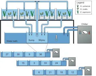
Figure 2. Experimental set-up showing three chilled water baths each with four randomly allocated sumps immersed within them. Each sump contained one of the 12 salinity treatments. Water was piped from the sump to the four replicate tanks and back again on closed-circulation.
[image:2.595.51.388.432.701.2]whereasH. ovalishas pairs of ovate leaves arising from the rhizome on petioles (Fig 1).
Zostera muelleri plants were collected from Pelican Banks,
Gladstone (23u45.8959S, 151u18.2449E) during low tide three
months before the experiments started. The plants were collected using a 10 cm corer, with sediment and rhizome and roots collected intact. The cores were placed in plastic-lined pots, the plastic bag sealed over the top of the seagrass with 2–3 cm of water
during transport to the experimental facility.Halodule uninervisand
H. ovalisplants were collected from Cockle Bay, Magnetic Island
(19u10.612S, 146u49.737E) using the same technique two months prior to the experiments. The plants were kept in 1000L aquaria at the Aquaculture facility in James Cook University on a closed
circulation system in seawater piped from Bowling Green Bay seawater intake under a 30% light-reducing roof.
[image:3.595.52.550.103.239.2]The experiment consisted of 12 salinity treatments, starting from 3 PSU and increasing by 3 PSU to 36 PSU (approximate marine seawater). Salinity treatments were obtained by diluting the seawater with de-chlorinated freshwater. Every salinity treatment consisted of four replicate tanks (65L KiTab clear plastic containers) with one pot of each species per tank (i.e. n = 4). All treatments started at 36 PSU and salinity was reduced by 25% each day over four days to the target treatment salinity to mimic the more gradual decline in salinities that occur during run-off events and to minimize potential impacts from shock osmotic changes. Throughout the experiment, salinity was measured every
Table 1.Results of single factor repeated measures analysis of variance (RM-ANOVA) for change in shoot density at salinity
treatments of 3 to 36 PSU in three seagrass species:Halophila ovalis,Halodule uninervisandZostera muelleri.
H. ovalis H. uninervis Z. muelleri
df F p df F p df F p
Within-subjects effects
Time 2.580 9.432 ,0.001 2.364 4.338 n.s. 3.131 78.380 ,0.001
Time x salinity 28.384 21.949 ,0.001 26.004 6.556 ,0.001 34.445 11.848 ,0.001 Between-subjects effects
Salinity 11 44.170 ,0.001 11 7.366 ,0.001 11 19.531 ,0.001
Transformations 4thRt (x+101) SqRt (x+101) SqRt (x+101)
Significance level (p) 0.01 0.01 0.01
Transformations performed to meet assumptions of ANOVA and significance level used for interpretation of results are also indicated for each species. doi:10.1371/journal.pone.0094014.t001
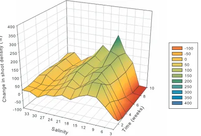
Figure 3. Change inHalophila ovalisshoot density relative to pre-treatment (week 0) (y-axis) as indicated by colour shading from
100% loss (red) through to 400% increase (blue), at salinities 3 to 36 PSU (x-axis) after 1 through to 10 weeks of exposure to
treatment salinity (z-axis).n = 4.
[image:3.595.55.460.425.700.2]1 to 3 days using a digital salinity/conductivity/temperature meter (YSI, model 63) and salinity was adjusted when necessary to maintain salinity within 0.5 PSU of target salinity. Plant responses to these salinities were monitored for 10 weeks. Previous salinity studies indicate that seagrass changes settle down by this time [5,12], and furthermore, this experimental duration is approxi-mately equal to or more likely exceeds the length of individual hypo-salinity events in the region.
The experiments were conducted outdoors during summer/ autumn months (February to April) when high ambient temper-atures occur, thus chilling units were installed to moderate temperature fluctuations within the treatment tanks throughout the experiment. There were three chilled freshwater baths (1000L tanks) that were cooled using external water chillers. Each of the 12 salinity treatments had one 60L sump (60L plastic bin) that was placed randomly in one of the 3 chilling baths, each bath containing 4 sumps (Fig 2). The chilled baths with sumps were held underneath tables that held the experimental tanks. From each sump, water with corresponding salinity was pumped into four replicate tanks resulting in a total of 48 tanks (4 replicate tanks
612 sumps/salinity treatments = 48 tanks in total). Each tank
contained one pot of each of the three species (48 tanks63
species/pots = 144 pots). Temperature was recorded every 30 mins using iBCod 22L model of iBTag in six randomly selected tanks for the duration of the experiment. Water temperature was
26uC on average and ranged from 22uC to 34uC reaching these
temperature extremes for short periods (1–2 h) on some days.
Nitrogen (N) as NH4Cl and phosphate (P) as KH2PO4were added
to the water column at very low concentrations to increase
concentrations within each system by 0.05mMol of P and
1.0mMol of N every 2 weeks. Nutrient concentration was
measured after six weeks and was found to be 0.8mMol (60.2)
NH3, 0.4mMol (60.1) NOx, and 0.2mMol (60.8) PO4. Average
light intensity under the 30% light-reducing roof was 17 mol
photons m22d21of Photosynthetically Active Radiation (PAR),
measured with an Odyssey 2Pi quantum sensor (Dataflow,
Odyssey photosynthetic recording system) recording every
30 mins throughout the experimental period. The tanks were periodically cleaned by syphoning out sediment and organic matter accumulating at the bottom of tanks and plants were inspected every week for signs of grazing by amphipods. Amphipods were removed to prevent an outbreak, which could lead to overgrazing of the plants. Although signs of grazing were observed at times, this cleaning regime was sufficient to avoid outbreaks.
Plant growth and survival
The number of shoots in each pot forZ. muelleriandH. uninervis,
or the number of leaf pairs forH. ovaliswere counted prior to the
experiment and then weekly during the first four weeks of the experiment and fortnightly from the sixth week up to and
including the tenth week. Change in shoot density (DSht) was
calculated as a percentage change in each week relative to pre-treatment for each individual replicate:
DSht~ ðSht tx{Sht t0Þ Sht t0
! "
|100 ð1Þ
whereDSht is change in shoot density, Shttxis shoot density at
time x (weeks 1 through to 10) and Sht t0is shoot density at week
zero (pre-treatment).
Leaf morphometrics (width and height) ofZ. muelleri,H. uninervis
and H. ovalisand number of leaves per shoot for the two blady
species were measured after 10 weeks at treatment salinity. These data were used to calculate foliar surface area (SA) as follows:
SA~shoot density|ðleaves per shootÞ{
0:5|leaf length|leaf width ð2Þ
for blady species (H. uninervis and Z. muelleri); and,
SA~leaf density|p| leaf length
2
# $
| leaf width
2
# $
ð3Þ
for the ovate speciesH. ovaliswhere SA is the foliar leaf area (cm2),
shoot density are leaves per experimental pot, leaves per shoot are the mean number of leaves (usually 1 to 4) per seagrass shoot and leaf length (cm) and leaf width (cm) of the youngest fully mature leaf. A half leaf was subtracted from the total number of leaves per shoot in calculating LA of blady species to account for one leaf on each shoot being in development and therefore not full sized [24].
Halophila ovaliswas the only species to flower throughout the
experimental period. Flowering had commenced prior to the initiation of the experiment and continued throughout. New leaf
pairs are produced inH. ovalisevery 3 or 4 days at experimental
water temperatures of approximately 27–27uC [25] andH. ovalis
[image:4.595.53.288.103.440.2]typically had 4 to 5 leaf pairs per branch. Flowering is initiated in
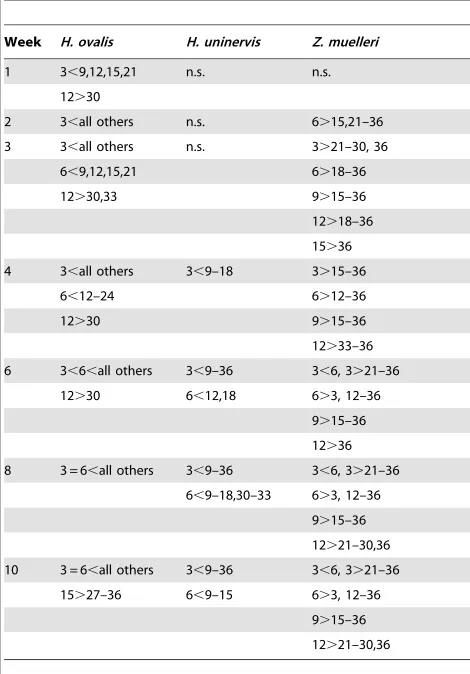
Table 2.Summary of Tukeys Post-hoc comparisons for each week for change in shoot density.
Week H. ovalis H. uninervis Z. muelleri
1 3,9,12,15,21 n.s. n.s.
12.30
2 3,all others n.s. 6.15,21–36 3 3,all others n.s. 3.21–30, 36
6,9,12,15,21 6.18–36
12.30,33 9.15–36
12.18–36 15.36 4 3,all others 3,9–18 3.15–36
6,12–24 6.12–36
12.30 9.15–36
12.33–36 6 3,6,all others 3,9–36 3,6, 3.21–36
12.30 6,12,18 6.3, 12–36 9.15–36 12.36 8 3 = 6,all others 3,9–36 3,6, 3.21–36
6,9–18,30–33 6.3, 12–36 9.15–36 12.21–30,36 10 3 = 6,all others 3,9–36 3,6, 3.21–36
15.27–36 6,9–15 6.3, 12–36 9.15–36 12.21–30,36
Differences among treatments are indicated for each species at each measuring time
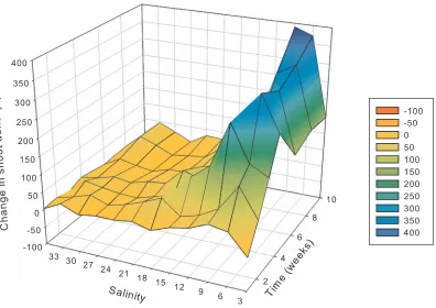
Figure 5. Change inZostera muellerishoot density relative to pre-treatment (week 0) (y-axis) as indicated by colour shading from 100% loss (red) through to 400% increase (blue), at salinities 3 to 36 PSU (x-axis) after 1 through to 10 weeks of exposure to
treatment salinity (z-axis).n = 4.
[image:5.595.60.456.422.702.2]doi:10.1371/journal.pone.0094014.g005
Figure 4. Change inHalodule uninervisshoot density relative to pre-treatment (week 0) (y-axis) as indicated by colour shading from
100% loss (red) through to 400% increase (blue), at salinities 3 to 36 PSU (x-axis) after 1 through to 10 weeks of exposure to
treatment salinity (z-axis).n = 4.
young leaf pairs, with more advanced reproductive structures away from the growing apex. Assuming a leaf pair production rate of 4 days, we conservatively assumed that all reproductive structures present after 4 weeks (28 d) were initiated under treatment conditions. We counted all reproductive structures (male and female flowers, as well as fruits) in each pot at weeks 4, 6, 8 and 10. We calculated reproductive potential – the highest number of reproductive structures occurring under treatment conditions as follows:
Reproductive potential~max R4½ ,R6,R8,R10$ ð4Þ
where R4 is mean structures in week 4 of treatment salinity
through to R10, which is mean structures in week 10. We also
present the total number of reproductive structures against shoot density for each replicate.
Leaf growth rate was measured in week 10 on the two blady
species (Z. muelleri and H. uninervis) using the leaf hole punch
method [26]. Holes were punched using a hypodermic needle in the top of the sheath of each shoot, and after 5–7 days we measured the distance between the mark in the sheath and the mark on the leaves. We aimed to measure up to 10 shoots per replicate pot, though the actual number measured in each pot was variable depending on shoot density and visibility of marks.
Statistical analyses
Shoot density data was analysed using a one-way repeated measures analysis of variance (RM ANOVA) with salinity as a fixed factor between-subjects effect and time (weeks) as the within-subjects effect. Data were first checked for homogeneity of variances using Levene’s test, and transformed if failing this assumption of ANOVA. Transformation was not successful at improving variances at all times, typically one or two measuring
times failed these tests (p,0.05) in which case the ANOVA was
[image:6.595.51.371.73.398.2]still performed on transformed data as the ANOVA is relatively robust to violations of assumptions in large experiments such as this; however, the significance level was set to 0.01 to minimize the risk of a Type II error [27]. Data were also checked for sphericity (correlations among time) and the degrees of freedom was adjusted using the Greenhouse-Geiser epsilon adjustment where necessary. Where a significant interaction between time and salinity was observed, post-hoc analyses to explore differences among treat-ments were performed for each measuring time separately. For single time data, single factor ANOVA’s were performed with salinity as a fixed factor. Data were tested and treated as described above, and post-hoc analyses were conducted using S-N-K comparisons. All statistical analyses were performed using SPSS v20.0. Key statistical results are described in text with detailed statistical results in Tables.
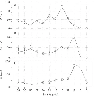
Figure 6. Foliar surface area (SA, cm2) calculated from shoot density, leaves per shoot and leaf length and width ofH. ovalis(A),H.
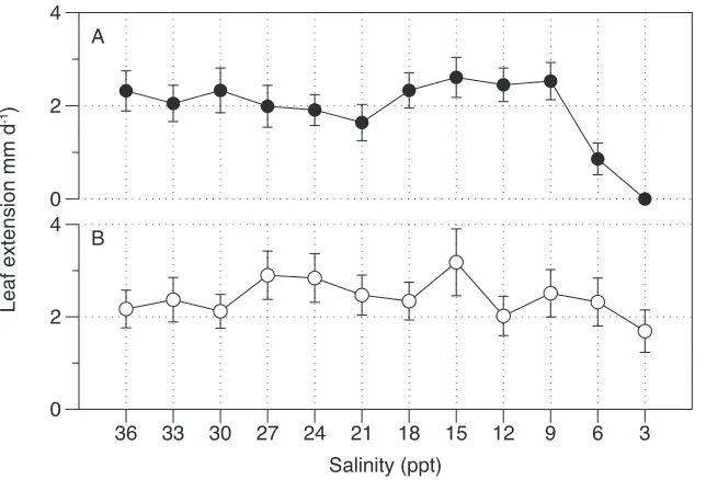
Figure 8. Leaf extension rate (mm d21) forH. uninervis(A) andZ. muelleri(B) after 10 weeks exposure to hypo-salinity.n = 46SE.
[image:7.595.51.373.499.718.2]doi:10.1371/journal.pone.0094014.g008
Figure 7. Sexual reproduction inHalophila ovalisunder salinity treatment conditions showing (A) reproductive potential which is
the highest mean (total number of flowers and fruits) recorded for each treatment in weeks 6–10; and, (B) reproductive output
(total number of flowers and fruits) correlated with shoot density at 10 weeks.n = 46SE.
Results
Shoot density
Initial shoot densities were on average 55 (6SE 8) leaf pairs for
H. ovalis, 8 (6SE 1) shoots forH. uninervisand 30 (6SE 5) shoots
forZ. muelleri. Changes in shoot density in response to hypo-salinity
generally followed the same trends among species with a salinity response that was affected by time (Table 1); however, thresholds and response times were variable. The most notable difference
among species was in their sensitivity at the lowest salinities;H.
ovalis was the most sensitive, whereas Z. muelleri was the most
tolerant of very low (3 and 6 PSU) salinities. Furthermore, Z.
muelleriincreased shoot density by the largest magnitude at
low-mid salinities.
More specifically, inH. ovalisleaf pair density had declined after
a one-week exposure to 3 PSU (Fig 3) and after 2 weeks it was
significantly (p,0.01) lower than all other salinity treatments
(Table 2). At the same time, leaf pair density showed an initial increase by 24% at 6 PSU after just 1 week, but reduced soon
afterwards with significant (p,0.01) reductions at 6 PSU
compared to low and mid salinities after 3 weeks. After 6 weeks there were no shoots remaining at 3 PSU and after 10 weeks there were just 3% remaining at 6 PSU. There was a very distinct threshold between 6 and 9 PSU, with leaf pair density increasing relative to starting density and being the highest at salinities
ranging from 9 to 15 PSU; however, significant (p,0.01) increases
in shoot density occurred only at 12 and 15 PSU. Shoot density increased at 36 and 33 PSU (by 30% and 55%), which was followed by negligible change in density at 30 PSU (2% increase), but density then increased again at lower salinities until reaching mortality thresholds.
ForH. uninervis, the general trends were similar but the reaction
time was slower and was more difficult to detect, as initial shoot density was considerably lower. There were no significant differences among treatments up to and including 3 weeks of
hypo-salinity exposure (Fig 4). After 4 weeks, density had significantly declined in 3 PSU relative to salinities of 9 through 18 PSU, and after 6 weeks density was significantly lower at 3 PSU than in all other treatments. After 10 weeks, there were no shoots
remaining at 3 PSU. At 6 PSU,H. uninervisinitially increased by
25% after 3 weeks, but started to decline thereafter, being significantly reduced relative to low/mid-range salinities after 4 weeks and there was 54% loss after 10 weeks. There was a distinct threshold between 6 and 9 PSU, with no net loss of shoots at 9 PSU, which instead showed the greatest increase in density among all salinities of 170% after 10 weeks.
InZ. muelleri, hypo-salinity had a significant and positive effect
on shoot density at salinities from 3 to 15 PSU (Fig 5). After 2
weeks, shoot density had increased significantly (p,0.01) more at
6 PSU compared to higher salinities, and after 3 weeks, density
had increased significantly (p,0.01) at salinities from 3 to 15 PSU
relative to higher salinities. After an initial increase of 240% at 3 PSU within 4 weeks, shoot density started to decline, but remained elevated relative to pre-treatment conditions throughout the experiment and was 150% greater than starting density after 10 weeks. The largest increase in shoot density was at 6 PSU, where density was 400% higher than pre-treatment after 10 weeks. It was
significantly (p,0.01) higher at 6 PSU than all other treatments
(except 9 PSU) after 4weeks and remained significantly (p,0.01)
elevated throughout. At 9 PSU, shoot density was significantly
(p,0.01) higher than all salinities of 15 PSU and greater after just
3 weeks. Shoot density was significantly (p,0.01) higher at 12 PSU
than at 21–36 PSU (except 33 PSU) after 8 and 10 weeks. The smallest change in shoot density occurred at 36 and 27 PSU, with 0 and 1% increase in shoot density, respectively, after 10 weeks.
Leaf area
Foliar surface area (SA), calculated from shoot density as well as shoot size (leaf length, width and leaves per shoot) after 10 weeks exposure to hypo-salinity treatments, followed the same general
trends and magnitude of response as for shoot density. For H.
ovalis, salinity had a significant effect (F = 42.041, MS = 37.236,
p,0.001, SqRt transformed) on SA. The largest SA occurred at
15 PSU, where it was significantly (p,0.01) higher than all other
treatments except 21 PSU, and was more than double that at 36 PSU (Fig 6A). The lowest SA occurred at 3 and 6 PSU where there were just 0 and 2 shoots remaining, resulting in a
significantly (p,0.001) reduced SA compared to all other
treatments. For H. uninervis salinity also had a significant effect
on SA (MS = 9.989, F = 6.839, p,0.001, SqRt transformation),
the peak in SA at 9 PSU was significantly (p,0.01) greater than
SA at 3-6 PSU, and 18–24 PSU, inclusive (Fig 6B). SA was
significantly (p,0.05) lower at 3 PSU than SA at all salinities
except 21 and 24 PSU. For Z. muelleri, the significant effect of
salinity on SA (MS = 25.711, F = 10.182, p,0.001, SqRt
trans-formation) peaked at 6 and 9 PSU, which were 5 times greater
than at 36 PSU, and which were both significantly (p,0.05)
higher than all other treatments (Fig 5C).
Sexual reproduction (flowering)
Reproductive potential, which is the highest mean recorded in weeks 4–10, increased with salinity, with no structures at 3–9 PSU
and the largest number (3.25 pot21) occurring at 36 PSU (Fig 7A).
This is in stark contrast to leaf pair density which was greatest at
12–15 PSU for H. ovalis. There was an anomaly of reduced
[image:8.595.51.277.74.233.2]reproductive effort at 30 and 33 PSU compared to higher and lower salinities. When plotted against leaf pair density (Fig 7B), the greatest number of reproductive structures occurred at low to moderate leaf pair densities, and at very high leaf pair densities
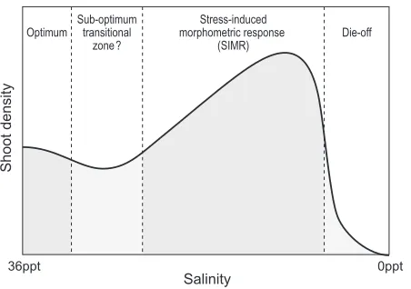
Figure 9. Conceptual summary of the seagrass responses to
hypo-salinity. High (marine, 36 PSU) salinities are ‘‘optimum’’, as
shoot density steadily increased throughout the experimental period at this salinity while sexual reproduction (forH. ovalis) was at its ‘‘peak’’. At slightly depressed salinities (30–33 PSU) there appeared to be a ‘‘sub-optimal’’ transition zone as shoot density showed minimal increase and, furthermore, sexual reproduction (forH. ovalis) was low. With further hypo-salinity (,30 PSU), a stress-induced morphometric response was associated with a re-prioritisation of resources that saw massively increased shoot density (and leaf area) and reduced sexual reproduc-tion. At extreme hypo-salinity (3–6 PSU) plant mortality occurred. The cut-off for each response phase moved to higher salinities with increased duration of exposure.
(.165 pairs per pot) there was no reproductive structures, nor at
very low densities (,50 pairs), where the plants were generally
dying.
Growth
Leaf growth (measured as leaf extension, mm d21) showed very
little response to the salinity treatments. H. uninervis was
significantly affected by the salinity (MS = 2.203, F = 7.955,
p,0.001, non-transformed, Fig 8A), but only at 3 and 6 PSU in
plants that were essentially dead or almost dead. Growth in 3 PSU was significantly lower than all other treatments, while growth at 6 PSU was significantly lower than 9–18 PSU and 30 PSU and 36
PSU, but not other treatments. Growth in Z. muelleri was also
significantly affected by salinity (MS = 0.720, F = 2.591 and
p,0.05, Fig 8B), with growth at 3 PSU being lower than 15
PSU only.
Discussion
These coastal Indo-Pacific seagrasses demonstrated very broad salinity tolerance when gradually exposed to hypo-salinity. Even
after 10 weeks exposure,Zostera muellerihad survived to salinities as
low as 3 PSU, whileHalophila ovalisandHalodule uninervisremained
abundant at 9 PSU. However, the plant-scale responses were complex, and the high treatment-resolution enabled us to develop a thorough conceptual model to describe this response (Fig 9). The most distinctive finding was a stress-induced morphometric response (SIMR) [20–22], characterised by shoot proliferation.
This corresponded to reduced flowering (for Halophila ovalis)
indicating a diversion of resources away from sexual reproduction to support the lateral branching. This did not come at the expense of leaf growth, which was largely unaffected by salinity, or shoot development (shoot size), as the foliar surface area mirrored the shoot density response. This shoot proliferation was a ‘moderate stress response’ and as the hypo-salinity treatments progressed to lower salinities, severe stress resulted in die-off (Fig 9). In this way, the shoot proliferation preceded mortality.
A ‘sub-optimal transitional zone’ between optimum salinity (36 PSU) and SIMR salinities appeared at 27–33 PSU depending on species, recognizable as a zone with small changes in shoot density (Figs 5 and 6). For example, the smallest change in shoot density
occurred at 30 PSU inH. ovalis(2%); while at salinities both above
(optimum salinity) and below this (stress response) there was shoot proliferation. There was also very low sexual reproduction in this transition zone. Previous studies have reported SIMR responses for other non-seagrass species groups [20–22]; however the proposed sub-optimal transitional zone requires further validation. The broad salinity tolerance indicates intracellular osmoregu-lation within the plant tissues. In halophytes, selective ion and solute accumulation enables high intra-cellular osmotic potentials to remain. A number of osmolytes occur in seagrass leaves,
including, inorganic ions (Na+, K+, Cl2) soluble sugars and amino
acids (in particular proline) [3]. Adjusting osmolyte concentration is energetically costly and slow, and this may partially explain why gradual changes in salinity, rather than sudden changes are associated with broad salinity tolerance [3]. Hypo-salinity can progress quickly: for example, sudden changes might result from heavy rainfall falling directly onto very shallow or even exposed intertidal meadows, or during very sudden and heavy run-off. Under these circumstances, the inability to slowly regulate osmolyte concentrations may cause more cellular damage and result in mortality at higher salinities [3,5,12].
Threshold salinities associated with mortality were different
among species with H. ovalis being the most sensitive, and Z.
muelleri the most tolerant of hypo-salinity. We have compared
salinity thresholds associated with sub-lethal and lethal impacts from this study with published findings (Table 3). This comparison focuses on mortality or changes in abundance. Since the studies summarized in the comprehensive review by Touchette [3] there has been considerable research effort exploring salinity stress, in particular physiological responses to hyper-salinity stress in
Thalassia testudinum (e.g. [5,17,28]) and Posidonia oceanica (e.g.
[18,29,30]). As summarized in Table 3 there are fewer data available on hypo-salinity responses, though where measured, seagrasses do tend to have low hypo-salinity thresholds (Table 3). This detailed experimental design has enabled us to identify salinity thresholds with a high level of precision. A significant outcome from this analysis is the identification of a stress-induced morphometric response indicated in Table 3 as a ‘‘sub-lethal’’ response. Furthermore, our exposure time has exceeded that of many previous studies enabling us to consider sensitivity of seagrasses over ‘wet season’ time-scales.
The question remains as to why these species tend to be restricted to waters that are predominantly marine when they are clearly tolerant of hypo-salinity. There are a number of possibilities. Firstly, this study was conducted over a 10-week period to represent a salinity flood event. Exposure to hypo-salinity for longer than 10 weeks could result in higher mortality rates. Secondly, low salinity events tend to coincide with elevated turbidity and nutrients as well as fast water flows. These other environmental impacts, or potentially synergistic impacts (for example, mortality increased with ammonium concentration in
Thalassia testudinum [11]) could prevent habitation in brackish,
riverine environments, rather than salinity itself. Thirdly, repro-ductive effort was severely impaired at low salinities – although this
could only be measured forH. ovalis. In some species (e.g.Ruppia
maritima), seedling germination is enhanced by rapid osmotic shock from hyper to hypo-salinity [31]; however, this study demonstrates that seed production, in these species was inhibited by chronic
exposure to hypo-salinity.Halophila ovalisis a colonizing species,
which is highly dependent on seed production for long-term survival and disruptions to sexual reproduction would probably prevent population survival. Furthermore, if seed production and germination are successful, seedling development is highly sensitive to small changes in salinity [32].
In conclusion, hypo-salinity stress caused a stress-induced morphometric response (SIMR) followed by severe mortality in
H. ovalisandH. uninervisat salinities less than 9 PSU. If observed in
natural conditions, a SIMR could suggest that the population is not only healthy, but is in fact in a trajectory of increasing abundance when using traditional monitoring tools, such as shoot density or percent cover. A critical next step is to explore how other interacting factors can affect responses to hypo-salinity.
Acknowledgments
We also thank the staff, in particular B. Lawes and S. Wever at the Marine and Aquaculture Research Facilities Unit at James Cook University for assistance with the experimental set-up. This work was undertaken on plants collected from the Great Barrier Reef World Heritage Area by the James Cook University Authorization MTB41.
Author Contributions
References
1. Les DH, Cleland MA, Waycott M (1997) Phylogenetic studies in Alismatidae, II: Evolution of marine angiosperms (seagrasses) and hydrophily. Syst Bot. 22: 443– 463.
2. Janssen T, Bremer K (2004) The age of major monocot groups inferred from 800+rbcL sequences. Bot J Linn Soc. 146: 385–398.
3. Touchette BW (2007) Seagrass-salinity interactions: Physiological mechanisms used by submersed marine angiosperms for a life at sea. J Exp Mar Biol Ecol. 350: 194–215.
4. Lirman D, Cropper WP, Jr. (2003) The influence of salinity on seagrass growth, survivorship, and distribution within Biscayne Bay, Florida: field, experimental, and modeling studies. Estuaries 26: 131–141.
5. Koch MS, Schopmeyer SA, Kyhn-Hansen C, Madden CJ, Peters JS (2007) Tropical seagrass species tolerance to hypersalinity stress. Aquat Bot. 86: 14–24. 6. Walker DI, Kendrick GA, McComb AJ (1988) The distribution of seagrass species in shark bay, Western Australia, with notes on their ecology. Aquat Bot. 30: 305–317.
7. Gacia E, Invers O, Manzanera M, Ballesteros E, Romero J (2007) Impact of the brine from a desalination plant on a shallow seagrass (Posidonia oceanica) meadow. Estuarine, Coastal and Shelf Science. 72: 579–590.
8. Furnas M (2003) Catchment and corals: terrestrial runoff to the Great Barrier Reef. Townville Queensland: Australian Institute of Marine Science. 334 p. 9. Preen AR, Long WJL, Coles RG (1995) Flood and cyclone related loss, and
partial recovery, of more than 1000 km2
of seagrass in Hervey Bay, Queensland, Australia. Aquat Bot. 52: 3–17.
10. Campbell SJ, McKenzie LJ (2004) Flood related loss and recovery of intertidal seagrass meadows in southern Queensland, Australia. Estuarine, Coastal and Shelf Science. 60: 477–490.
11. Kahn AE, Durako MJ (2006)Thalassia testudinumseedling responses to changes in salinity and nitrogen levels. J Exp Mar Biol Ecol. 335: 1–12.
12. Griffin NE, Durako MJ (2012) The effect of pulsed versus gradual salinity reduction on the physiology and survival ofHalophila johnsoniiEiseman. Marine Biology. 159: 1439–1447.
13. Fernandez-Torquemada Y, Sanchez-Lizaso JL (2011) Responses of two Meditteranean seagrasses to experimental changes in salinity. Hydrobiologia. 669: 21–33.
14. Chaves MM, Flexas J, Pinheiro C (2009) Photosynthesis under drought and salt stress: regulation mechanisms from whole plant to cell. Annals of Botany. 103: 551–560.
15. Munns R, Tester M (2008) Mechanisms of salinity tolerance. Annu Rev Plant Biol. 59: 651–681.
16. Ralph P (1998) Photosynthetic responses ofHalophila ovalis(R. Br.) Hook.f. to osmotic stress. J Exp Mar Biol Ecol. 227: 203–220.
17. Howarth JF, Durako MJ (2013) Variation in pigment content of Thalssia testudinumseedlings in response to changes in salinity and light. Bot Mar. 56: 261–273.
18. Sandoval-Gil J, Marı´n-Guirao L, Ruiz J (2012) Tolerance of Mediterranean seagrasses (Posidonia oceanicaandCymodocea nodosa) to hypersaline stress: water relations and osmolyte concentrations. Marine Biology. 159: 1129–1141. 19. Marı´n-Guirao L, Sandoval-Gil JM, Bernardeau-Esteller J, Ruı´z JM,
Sa´nchez-Lizaso JL (2013) Responses of the Mediterranean seagrassPosidonia oceanicato hypersaline stress duration and recovery. Mar Environ Res. 84: 60–75. 20. Potters G, Pasternak TP, Guisez Y, Palme KJ, Jansen MAK (2007)
Stress-induced morphogenic responses: growing out of trouble? Trends Plant Sci. 12: 98–105.
21. Potters G, Pasternak TP, Guisez Y, Jansen MAK (2009) Different stresses, similar morphogenic responses: integrating a plethora of pathways. Plant, Cell & Environment. 32: 158–169.
22. Zolla G, Heimer YM, Barak S (2010) Mild salinity stimulates a stress-induced morphogenic response inArabidopsis thalianaroots. J Exp Bot. 61: 211–224. 23. Waycott M, McMahon K, Mellors J, Calladine A, Kleine D (2004) A guide to
tropical seagrasses of the Indo-West Pacific. Townsville: James Cook University. 72 p.
24. Collier CJ, Waycott M, Giraldo-Ospina A (2012) Responses of four Indo-West Pacific seagrass species to shading. Mar Pollut Bull. 65: 342–354.
25. McMahon KM (2005) Recovery of subtropical seagrasses from natural disturbance. Brisbane: The University of Queensland. 198 p.
26. Short FT, Duarte CM (2001) Methods for the measurement of seagrass growth and production. In: Short FT, Coles R, editors. Global seagrass research methods. Amsterdam: Elsevier Science. pp. 473.
27. Underwood AJ (1997) Experiments in ecology: Their logical design and interpretation using analysis of variance. Cambridge: Cambridge University Press.
28. Jiang Z, Huang X, Zhang J (2013) Effect of nitrate enrichment and salinity reduction on the seagrassThalassia hemprichiipreviously grown in low light. J Exp Mar Biol Ecol. 443: 114–122.
29. Marı´n-Guirao L, Ruiz JM, Sandoval-Gil JM, Bernardeau-Esteller J, Stinco CM, et al. (2013) Xanthophyll cycle-related photoprotective mechanism in the Mediterranean seagrassesPosidonia oceanicaandCymodocea nodosaunder normal and stressful hypersaline conditions. Aquat Bot. 109: 14–24.
30. Ruiz JM, Marin-Guirao L, Sandoval-Gil JM (2009) Responses of the Mediterranean seagrassPosidonia oceanicatoin situsimulated salinity increase. Bot Mar. 52: 459–470.
31. Strazisar T, Koch MS, Madden CJ, Filina J, Lara PU, et al. (2013) Salinity effects onRuppia maritima L. seed germination and seedling survival at the Everglades-Florida Bay ecotone. J Exp Mar Biol Ecol. 445: 129–139. 32. Kirkman H, Kuo J (1990) Pattern and process in southern Western Australian
seagrasses. Aquatic Botany. 37: 367–382.
33. Walker DI, McComb AJ (1990) Salinity response of the seagrassAmphibolis antarctica(Labill.) Sonder et Aschers.: an experimental validation of field results. Aquat Bot. 36: 359–366.
34. Walker DI (1985) Correlations between salinity and growth of the seagrass
Amphibolis antarctica(labill.) Sonder ex Aschers., In Shark Bay, Western Australia, using a new method for measuring production rate. Aquat Bot. 23: 13–26. 35. Pages JF, Perez M, Romero J (2010) Sensitivity fo the seagrassCymodocea nodosato
hypersaline conditions: a microcosm approach. J Exp Mar Biol Ecol. 386: 34– 38.
36. Sandoval-Gil JM, Marı´n-Guirao L, Ruiz JM (2012) The effect of salinity increase on the photosynthesis, growth and survival of the Mediterranean seagrassCymodocea nodosa. Estuarine, Coastal and Shelf Science. 115: 260–271. 37. Kahn A, Durako MJ (2008) Photophysiological responses ofHalophila johnsoniito
experimental hyposaline and hyper-CDOM conditions. J Exp Mar Biol Ecol. 367: 230–235.
38. Torquemada YF, Durako MJ, Lizaso JLS (2005) Effects of salinity and possible interactions with temperature and pH on growth and photosynthesis ofHalophila johnsoniiEiseman. Marine Biology. 148: 251–260.
39. Hillman K, McComb AJ, Walker DI (1995) The distribution, biomass and primary production of the seagrassHalophila ovalisin the Swan/Canning Estuary, Western Australia. Aquat Bot. 51: 1–54.
40. Ferna´ndez-Torquemada Y, Sa´nchez-Lizaso JL (2005) Effects of salinity on leaf growth and survival of the Mediterranean seagrassPosidonia oceanica(L.) Delile. J Exp Mar Biol Ecol. 320: 57–63.
41. Marı´n-Guirao L, Sandoval-Gil JM, Ruı´z JM, Sa´nchez-Lizaso JL (2011) Photosynthesis, growth and survival of the Mediterranean seagrassPosidonia oceanicain response to simulated salinity increases in a laboratory mesocosm system. Estuarine, Coastal and Shelf Science. 92: 286–296.
42. Adams JB, Bate GC (1994) The tolerance to desiccation of the submerged macrophytesRuppia cirrhosa(Petagna) grande andZostera capensissetchell. J Exp Mar Biol Ecol. 183: 53–62.
43. Koch MS, Schopmeyer SA, Holmer M, Madden CJ, Kyhn-Hansen C (2007)