Stellar Feedback, AGN Feedback and Fluid Microphysics in Galaxy Evolution

(1)

in Galaxy Evolution

Thesis by

Kung-Yi Su

In Partial Fulfillment of the Requirements for the Degree of

Doctor of Philosophy

CALIFORNIA INSTITUTE OF TECHNOLOGY Pasadena, California

2019

(2)

Kung-Yi Su

ORCID: 0000-0003-1598-0083

(3)

ACKNOWLEDGEMENTS

First, I would like to thank my advisor, Philip Hopkins, who literally picked me up at the lowest point of my life. When I switched fields in the fourth year of my Ph.D. study, Phil took me into the group, and bear with my ignorance. He not only provided academic, research, and career advice, but is also more than generous in sharing the credit, promoting my work, and supporting my trips. I feel lucky for having such an advisor and mentor whom I would not hesitate going to whenever I need advice. Phil set an exceptionally great example and high standards, with his broad knowledge in each sub-field of galaxy formation, sharp physical intuition, and extremely high efficiency. I will always look up to these attributes.

I also thank Chris Hayward, with whom I collaborated for all my thesis work. Chris helped me tremendously not only in developing and defining the projects, but also in numerous other aspects, especially during the first year after I switched fields. As I will become Chris’s colleague at the CCA, Flatiron Institute, I look forward to our continued collaboration.

Moreover, I appreciate all the fellow graduate students in Phil’s group, especially Xiangcheng Ma and Matt Orr. Xiangcheng, being the first student of Phil, was frequently bothered by me with all sorts of questions I had, and always provided me with timely help. Matt Orr, being also my officemate, proof-read almost everything I wrote, and is probably the person I chatted/discussed with the most frequently.

I feel very blessed to be in the Feedback in Realistic Environments (FIRE) col-laboration, in which I can do cutting-edge physics research with state-of-the-art simulations, building on the great achievements and developments of Phil and the others. I feel fortunate to discuss and work with the greatest scientists, includ-ing Chris Hayward, Eliot Quataert, Dušan Kereš, Claude-André Faucher-Giguère, Daniel Anglés-Alcázar, Michael Boylan-Kolchin, Shea Garrison-Kimmel, Coral Wheeler, Cameron Hummels, Paul Torrey, Andrew Wetzel, Suoqing Ji, Victor Rob-les, TK Chan, and all the others. I especially thank Chris, Dušan, Shea, Claude, and Eliot for all their help and support during my job application.

I also thank the other faculty members at Caltech and elsewhere whom I have interacted with, especially my thesis committee members, Chuck Steidel, Evan Kirby, and Chris Martin.

(4)

legislation and the funding flexibility, which made it possible for me to switch fields even in the fourth year of my graduate study. I also thank the administrative staff, especially JoAnn in TAPIR and Daniel and Laura in ISP for all the prompt help.

Throughout the eight years of my graduate study in Caltech, I was fortunate to have lots of friends around to enjoy life outside of work. I owe my special thanks to Shun-Jia and Min-Feng for being with me thick and thin during my graduate study. I also thank Yun-Ting, Ying-Hsuan, Yu-Li, Hsiao-Yi, Linhan, Nien-En, Sunny, Chia-Hsien, Han-Hsin, Felix, Ying-Yu, Yen-Yung, Vincent, Mike, Jenny, Jill, and the Wu family for enduring friendships. I would especially like to single out Shu-Heng Shao, my lifetime best friend and 6th cousin according to 23andMe, for all the encouragement and support during my hardest time.

(5)

(6)

ABSTRACT

Understanding how the baryonic physics affects the formation and evolution of galax-ies is one of the most critical questions in modern astronomy. Significant progress in understanding stellar feedback and modeling them explicitly in simulations have made it possible to reproduce a wide range of observed galaxy properties. However, there are still various pieces of missing physics and uncertainties in galaxies of different mass range.

In this thesis, I will explore these missing pieces in baryonic physics on top of the Feedback in Realistic Environments (FIRE) stellar feedback in the cosmological hydrodynamic zoom-in simulations (FIRE-2 suite) and isolated galaxy simulations. These high-resolution simulations with FIRE physics capture multi-phase realistic interstellar medium (ISM) with gas cooling down to 10K, and star formations in dense clumps in giant molecular clouds. They are, therefore, an ideal tool for investigating the missing pieces in baryonic physics.

In the first part of the thesis,Chapter 2, I will focus on the discrete effects of stellar feedback like individual supernovae, hypernovae, and initial mass function (IMF) sampling in dwarfs (109−1010M). These discrete processes of stellar feedback can have maximum effects on the small galaxies without being averaged out. I will show that the discretization of supernovae (SNe) is absolutely necessary, while the effects from IMF sampling and hypernovae (HNe) is not apparent, due to the strong clustering nature of star formation.

In the second part of the thesis,Chapter 3 - 4, I will focus on fluid microphysics, exploring their effects on galaxy properties and their interplay with stellar feedback in sub-L* galaxies. I will demonstrate that, once the stellar feedback is explicitly implemented as FIRE stellar feedback model, fluid microphysics such as magnetic fields, conduction, and viscosity only have minor effects on the galaxy properties like star formation rate (SFR), phase structure, or outflows. Stellar feedback also strongly alters the amplifications and morphology of the magnetic fields, resulting in much more randomly-oriented field lines. However, despite the stellar feedback, the amplification of magnetic fields in ISM gas is primarily dominated by flux-freezing compression.

(7)

(8)

PUBLISHED CONTENT AND CONTRIBUTIONS

K.-Y. Su, P. F. Hopkins, C. C. Hayward, C.-A. Faucher-Giguère, D. Kereš, X. Ma, and V. H. Robles. Feedback first: the surprisingly weak effects of magnetic fields, viscosity, conduction and metal diffusion on sub-L∗galaxy formation. MNRAS, 471:144–166, October 2017. doi: 10.1093/mnras/stx1463.

K.-Y. Su, C. C. Hayward, P. F. Hopkins, E. Quataert, C.-A. Faucher-Giguère, and D. Kereš. Stellar feedback strongly alters the amplification and morphology of galactic magnetic fields. MNRAS, 473:L111–L115, January 2018a. doi: 10.1093/mnrasl/slx172.

K.-Y. Su, P. F. Hopkins, C. C. Hayward, X. Ma, C.-A. Faucher-Giguère, D. Kereš, M. E. Orr, and V. H. Robles. The failure of stellar feedback, magnetic fields, conduction, and morphological quenching in maintaining red galaxies. MNRAS, in press, arXiv:1809.09120, September 2018b.

Kung-Yi Su, Philip F. Hopkins, Christopher C. Hayward, Claude-André Faucher-Giguère, Dušan Kereš, Xiangcheng Ma, Matthew E. Orr, T. K. Chan, and Victor H. Robles. Cosmic Rays or Turbulence can Suppress Cooling Flows (Where Thermal Heating or Momentum Injection Fail). arXiv e-prints, art. arXiv:1812.03997, December 2018c.

Kung-Yi Su, Philip F. Hopkins, Christopher C. Hayward, Xiangcheng Ma, Michael Boylan-Kolchin, Daniel Kasen, Dušan Kereš, Claude-André Faucher-Giguère, Matthew E. Orr, and Coral Wheeler. Discrete effects in stellar feedback: Indi-vidual Supernovae, Hypernovae, and IMF Sampling in Dwarf Galaxies.MNRAS, 480(2):1666–1675, October 2018d. doi: 10.1093/mnras/sty1928.

(9)

LIST OF ILLUSTRATIONS

Number Page

1.1 The predicted stellar mass function without stellar feedback. . . 1 2.1 Stellar mass, SFR, the mass outflow rate, and the outflow

mass-loading factor as a function of time. . . 16 2.2 Gas density distributions for m10q in different phases and at different

redshifts. . . 18 2.3 Gas density distributions for m10v and m09 runs in different phases

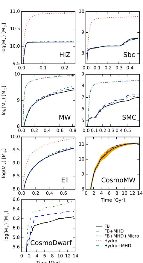
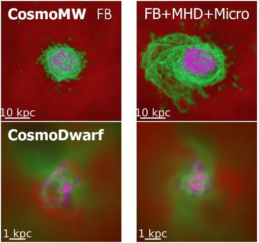
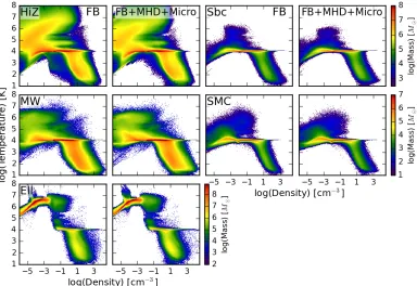
and at different redshifts. . . 19 2.4 Photon escape fractions (Qesc/Qint) for the m10q and m10v cases. . . 20 3.1 Star formation rates (SFRs) as a function of time. . . 42 3.2 Total stellar mass as a function of time. . . 43 3.3 Images of the gas morphology of the isolated galaxies with feedback. 45 3.4 Images of the gas morphology of the isolated galaxies without feedback. 46 3.5 Images of the gas morphology of the cosmological simulations atz= 0. 47 3.6 Temperature-density phase distribution of the isolated galaxy

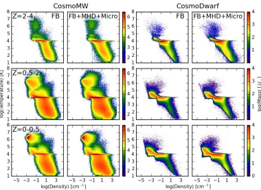
simu-lations. . . 48 3.7 Temperature-density phase distribution of the cosmological simulation. 49 3.8 Radial distributions of temperature, gas density and metallicity for

the cosmological runs averaged over the redshift rangez ∼0−0.07. . 50 3.9 Density distribution of gas in different phases. . . 51 3.10 Gas density distribution in different phases for the cosmological

sim-ulations averaged in different redshift intervals. . . 52 3.11 The total turbulent kinetic energy and magnetic energy per unit mass

of the non-outflowing disc gas in our simulations as a function of time. 56 3.12 The rms magnetic field strength of all and the cold (T < 8000 K)

component of the non-outflowing disc gas in our simulations as a function of time. . . 57 3.13 Distributions of the radial velocities of the gas particles in the isolated

galaxy simulations. . . 58 3.14 Distributions of the radial velocities of the gas particles in the

(12)

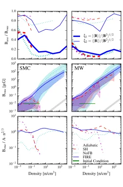
4.1 Edge-on and face-on projections of the gas density and magnetic field lines of the simulated galaxies. . . 73 4.2 The orderliness of magnetic fields and magnetic field strength as a

function of gas density. . . 75 4.3 The rms magnetic field strength, magnetic energy, and turbulent

energy as a function of time. . . 76 5.1 The X-ray luminosity (0.5-7 keV) of our initial conditions and the

average luminosity of the last 100 Myr of each run plotted on the X-ray luminosity - halo mass plane in comparison to the observations. 90 5.2 Cooling flows in different phases as a function of time: The baryonic

mass variation, hot gas (> 106 K) mass, warm gas (8000−106 K) mass, and cold gas (< 8000 K) mass within 30 kpc. . . 91 5.3 Specific SFR, SFR, and SFRs from gas initially at radii larger than

25 kpc (fueled by cooling flow). . . 94 5.4 Cooling time and ratio of cooling time to dynamical time of gas hotter

than 105K. . . 96 5.5 Energy input, cooling, SNe and AGB winds energy input rate as a

function of time. . . 97 5.6 The comparisons of thermal, magnetic, CR and turbulent energy per

unit mass, averaged over the 90-100th Myr. . . 98 5.7 The SFR of m12 runs with different core gas density within 10 kpc. . 99 5.8 The effective fraction of Spitzer conductivity, as a function of radius. 103 6.1 Energy and momentum input rate per unit logarithmic galacto-centric

radius logr (time-averaged over the last 100 Myr of each run), in a subset of our halom14runs. . . 120 6.2 Baryonic mass within 30 kpc (excluding pre-existing stars from the

ICs), SFRs, SFRs from gas which was at r > 25 kpc, and Specific SFRs as a function of time. . . 122 6.3 Density, temperature, and entropy profiles as a function of radius. . . 124 6.4 The face-on projected density and average temperature of the more

successful runs. . . 125 6.5 X-ray cooling luminosity LX, integrated from 0.5−7 keV. . . 126 6.6 1D rms Mach number and 1D rms velocity dispersion as a function

of radius. . . 127 6.7 Gas cooling time and cooling time over dynamical time as a function

(13)

6.8 Cumulative (integrated inside< r) cooling rate (EÛcool), total feedback energy input rate (EÛinput), and difference (net loss/gain), in the runs from Fig. 6.3 averaged over their last 100 Myr. . . 131 6.9 Testing “rejuvenation”: The SFRs of runs restarted with and without

turbulent stirring from different time of ‘Turb-core-5’. . . 132 6.10 Cumulative cooling rate versus energy input (as Fig. 6.8, but including

onlystellar feedback from old stellar populations in theEÛinputbudget),

of the “restarted” runs in Fig. 6.9. . . 133 6.11 Galaxy SFRs (as Fig. 6.2) in our suite of simulations of different mass

haloes (Table 6.3). . . 136 6.12 Density, temperature, & entropy profiles (as Fig. 6.3) averaged over

the last∼100 Myr of each run for the runs in Fig. 6.11. . . 137 6.13 Cumulative energy input vs. cooling (as Fig. 6.8) for the simulations

in Fig. 6.11. . . 138 6.14 An example of what happens to rapidly cooling gas in the turbulent

stirring runs which suppress cooling flows. . . 140 6.15 Comparison of energetics in ourm14cosmic ray runs. Comparison of

differential per-unit-radius (d_EÛ_/_d

logr) and cumulative (EÛ(< r)) gas cooling rates versus CR heating rates. Comparison of gravitational acceleration and the acceleration from the CR pressure gradient. . . . 141 7.1 Gas temperature and density under different Jet model. . . 150 A.1.1 Comparison of the total stellar mass, SFR, outflow rate, and outflow

mass loading of the m10q“IMF-SMP” runs with different resolutions. 173 A.1.2 Comparison of the photon escape fractions of the m10q “IMF-SMP”

runs with different resolutions. . . 174 A.1.3 Gas density distributions for m10q “IMF-SMP” runs with different

resolutions. . . 175 A.2.1 Resolution study of the SFR of the SMC model with “FB+MHD+Micro”.176 A.2.2 Resolution study of the density distribution of gas in different phases

in the SMC model with “FB+MHD+Micro”.. . . 177 A.2.3 Convergence of the radial velocity distribution of the gas particles in

the SMC model with “FB+MHD+Micro”. . . 177 A.2.4 The total turbulent kinetic energy and magnetic energy per unit mass

(14)

A.3.1 The comparison of (a) core (< 30kpc) baryonic mass, (b) hot gas (> 106K) mass, (c) warm gas (8000 − 106K) mass, (d) cold gas (< 8000K) mass, and (e) stellar mass, for ‘Default’ m14 runs at different resolutions. . . 179 A.3.2 Comparison of total SFR, and SFR from gas initially outside 25kpc,

for ‘Default’ m14 runs with different resolutions. . . 180 A.3.3 Cooling time, and cooling time over dynamical time, as a function of

radius for gas hotter than 105K for ‘Default’ m14 runs with different resolutions. . . 180 A.3.4 The cooling and energy input rates within 30 kpc and X-ray luminosity

in the 0.5−7 kev band for ‘Default’ m14 runs with different resolutions.181 B1 SFR (as Fig. 6.2) in our ‘Default’ and ‘Turb-core-1’m14runs,

(15)

LIST OF TABLES

Number Page

2.1 Galaxy models in Chapter 2 . . . 11

4.1 Physics variations in our simulation suite in Chapter 4 . . . 72

5.1 Galaxy models in Chapter 5. . . 92

5.2 List of runs with different physics variations in Chapter 5 . . . 93

6.2 Physics variations (run at highest resolution) in our halo-m14survey . 119 6.3 Physics variations (run at highest resolution) in our survey of lower-mass (m12&m13) haloes . . . 134

7.1 Parameters for the preliminary suite of jet simulations. . . 149

A.1.1 Particle resolutions used in our convergence tests for the default m10q run in Chapter 2 . . . 173

(16)

C h a p t e r 1

INTRODUCTION

Baryons, only contributing to∼ 16−17% (Jarosik et al.,2011) of the matter in the universe, is the key to understand the evolution of galaxies. Traditional dark matter only simulations, which only include gravity and assume that the baryonic mass follows the dark matter mass simply fail the galaxy mass function and the stellar mass–halo mass relations. As shown in Fig. 1.1, too many stars are formed, and the total stellar mass is significantly over-predicted especially in the most massive galaxies and the dwarfs. Simulations without strong stellar feedback also face similar challenges (Bournaud et al.,2010,Dobbs et al.,2011,Harper-Clark & Murray,2011, Hopkins et al.,2011,Krumholz et al.,2011,Tasker,2011).

Moreover, dark-matter-only simulations (cold dark matter) also predict other results contradicting to the observations, e.g., too many satellites (e.g., Kauffmann et al., 1993,Klypin et al.,1999,Moore et al.,1999), much denser galactic cores with cuspy

profiles (Amorisco et al. 2014,Flores & Primack 1994,Kuzio de Naray et al. 2008, Ogiya & Burkert 2015, Oh et al. 2008, Salucci et al. 2012, Walker & Peñarrubia

2011,de Blok et al. 2008, but seeStrigari et al. 2014), etc.

(17)

1.1 Important baryonic physics in galaxy evolution

Rapid progress has been made in the last decade in modeling baryonic physics, especially stellar feedback, in galaxy simulations (see e.g.,Agertz & Kravtsov,2016, Ceverino & Klypin, 2009, Governato et al., 2007, Hopkins et al., 2011, 2012a,b,

Uhlig et al., 2012). Explicitly modeling stellar feedback in simulations (Hopkins

et al.,2011,2012a,Hu et al.,2016,2017,Richings & Schaye,2016) can result in a

self-regulated multi-phase ISM, with giant molecular clouds (GMCs) turning only a few percent of their mass into stars in a dynamical time, and SFRs in agreement with observations (Hopkins et al.,2012b,2013a,d). Cosmological zoom-in simulations in the FIRE1 (Feedback In Realistic Environments) suite (Hopkins et al., 2014), especially, have been shown to be able to reproduce a wide range of observations, including star formation histories (Hopkins et al., 2014), the Kennicutt-Schmidt relation (Orr et al., 2018), the star-forming “main sequence” and time-variability of star formation (Sparre et al., 2017), galactic winds (e.g., Anglés-Alcázar et al., 2017b,Muratov et al.,2015,2017), the dense HI content of galaxy haloes

(Faucher-Giguère et al.,2015,2016,Hafen et al.,2017), the implied photon escape fractions of

high-redshift galaxies (Ma et al.,2016b), and galaxy metallicities (Ma et al.,2015a). I will briefly discuss the essential pieces of baryonic physics in the following.

1.1.1 Gas heating and cooling

As gas accretes onto the galaxies, accretion shocks can heat the gas up to the viral temperature. Other heating sources include Compton heating, photoionization and photoelectric heating from stars, black hole, and ionizing background. The reionization is the primary cause of the quenching of the ultra-faint dwarfs (Bullock et al., 2000). Finally, there is also cosmic rays and shock heating from supernovae

and AGN feedback.

On the other hand, various cooling mechanisms have to cool down the gas before they can fall into the galactic core and form stars. Important terms include bremsstrahlung for hot gas (> 106K), metal-line cooling and atomic cooling for warm gas (104−106 K), and fine-structure lines, molecular, and dust cooling for cold gas (< 104K).

1.1.2 Star formation

As the gas cools down, gravitational instabilities result in the gas fragmentation and the formation of the supersonically turbulent self-gravitating GMCs in the ISM. The fragmentation continues until the scale of proto-star. The initial stellar mass follows

1

(18)

initial mass function.

In FIRE, self-gravitating molecular gas denser than 1000cm−3 is allowed to form stars in a free-fall time. Although stars form in a free-fall time, stellar feedback quickly disrupts the GMC allowing only ∼ 1% of the gas to form stars. The star particles in the simulations are treated as single stellar populations followingKroupa (2002) IMF.

1.1.3 Stellar feedback

Through the life of a star, its feedback injects energy and momentum to the sur-rounding gas through the following mechanism: (1) Photo-heating: The photons from stars ionize and heat up the surrounding gas through photoionization and pho-toelectric heating. (2) Radiation pressure: The photons absorbed by dust grains also deposit photon momentum to the gas. (3) Supernovae: SN Types II or Ia generates a Sedov-Talor blast waves depositing 1051 erg to the surrounding gas. (4) Stellar winds: Stellar mass losses with continuously injected mass, metals, energy, and momentum from OB and AGB winds. Stellar feedback can effectively regulate the star formation for any galaxy. 1012M, and results in a realistic multi-phase ISM.

1.2 Uncertainties from other baryonic physics

Explicitly modeling the aforementioned gas cooling/heating, star formation and stellar feedback in cosmological zoom-in simulations (FIRE) has reached great success in reproducing a wild range of galactic properties and scaling relations. However, there are still various uncertainties and open questions in baryonic physics and how they affect galaxy evolution. In the following, I will address the points that will be the main focus of this theses.

1.2.1 How the discrete effect of stellar feedback affects dwarfs

Despite the success of stellar feedback, certain discrete stellar feedback processes still have uncertain effects on dwarfs, where the potential well is shallow, and the total number of stars is low. The following are the two major points that will be discussed inChapter 2.

The star to star variation in stellar feedback

(19)

photons, and radiation pressure coming from massive O stars. When galaxies are sufficiently massive, these effects should average out, but in dwarfs, in particular, failure to account for these fluctuations could lead to biased predictions for galaxy properties. This is certainly the case for measurements of e.g., the ionizing flux and spectral shapes of such systems (seeKrumholz et al., 2015,da Silva et al., 2012). IMF sampling gets more important when the mass resolution increases, and the baryonic particle mass fall below∼ 104M (Hensler et al.,2016, Hu et al., 2017). In such cases, the IMF is poorly sampled in a single star particle.

Super-energetic stellar feedback event: Hypernovae

HNe are core-collapse SNe that have energies that exceed the typical SN energy (∼ 1051erg) by a factor of 10 or more (E >1052erg;Nomoto et al. 2004,Podsiadlowski et al. 2004). Such extreme events could potentially blow out all the gas in a dwarf

galaxy, consequently completely quenching star formation if the dark matter halo is too low-mass to accrete further gas post-reionization. Whether or not an HNe quenches star formation determines whether its yield products can be incorporated into next-generation stars, which in turn determines whether or not the yield products of HNe should be observable.

1.2.2 The role of fluid microphysics in galaxies

Fluid microphysics such as magnetic fields, conduction and viscosity are not always included in galaxy simulations but can potentially affect various galactic properties. In Chapter 3, I will discuss their effects in a wide range of sub-L* galaxies. In Chapter5, I will explore whether fluid microphysics especially magnetic fields and conduction can help suppress the cooling flows (§ 1.2.3).

Magnetic fields

The tiny magnetic field seeded in the early universe is amplified by cosmic struc-ture formation and by magnetic dynamos in the ISM or circum-galactic medium (CGM). However, there are uncertainties on what the dominant field amplification mechanism is in the galaxies and whether stellar feedback affects the whole picture. These will be explored inChapter 4.

(20)

pressure can provide extra support, thus slowing down in-falling or collapsing of gas at various scale and suppressing the star formation. Magnetic fields can also be relevant because of their effects on fluid mixing instabilities, including the Rayleigh-Taylor (RT) and Kelvin-Helmholtz (KH) instabilities (Armillotta et al., 2017, Jun et al.,1995,McCourt et al., 2015). These instabilities can potentially affect galaxy

evolution through processes including the evolution of supernovae (SN) remnants (Jun & Jones,1999, Jun & Norman,1996a,b,Kim & Ostriker,2015b, Thompson, 2000) and AGN bubbles.

Conduction

Thermal conduction, which in the presence of magnetic fields is highly anisotropic, affects the stability of plasmas at both galactic and cluster scales (Armillotta et al., 2017,Choi & Stone,2012,Parrish et al.,2012b,Sharma et al.,2009,2010) and the

survival and mixing of multi-phase fluids. Combined with the effect of magnetic fields, conduction may be critical to determine the survival of cool clouds in galactic winds.

Due to the strong temperature dependence of the conductivity, conduction is ex-pected to have maximum effect in the hot halo of the massive galaxies and clusters. It can transport heat to the inner cool core and potentially suppress the inflow of the gas.

Viscosity

Viscosity has been more extensively studied in simulations of galaxy clusters. It has been suggested that viscosity can affect the turbulent motion of the intracluster medium (ICM) or CGM and affect the KH stability of various structures in the ICM (Markevitch & Vikhlinin,2007). It has been shown in particular that viscosity may be important for the dynamics of bubbles in the ICM inflated by AGN feedback or bursts of SNe activity (Reynolds et al.,2005,Sijacki & Springel,2006).

1.2.3 Cooling flow problem in massive galaxies

(21)

and presumably forming stars. This discrepancy is known as the “cooling flow prob-lem”. How to suppress the cooling flows and SFRs are the essential missing pieces in the evolution of massive galaxies. I will present the solutions not associated with an AGN inChapter 5, and those related to AGN feedback inChapter 6.

Non-AGN feedback solutions

Given that stellar feedback kicks and heats up the surrounding gas, conduction transports heat from the outer hot halo to the inner cool-core, and that magnetic fields provide extra pressure support, they can all possible suppress the cooling flows.

Martig et al.(2009) andDekel et al.(2009) described another scenario they referred to as “morphological quenching,” whereby quenching could be accomplished (SF suppressed) simply by altering a galaxy’s morphology. Specifically, they argued that turning a stellar disk into a more gravitationally stable spheroid would raise the Toomre-Qand stabilize the gas against fragmentation/star formation.

Cosmic rays

Cosmic rays (CRs) are the results of shocks, which accelerate protons to > GeV. Structure formation, supernovae, and AGN feedback can all generate cosmic rays. Roughly 10% of the supernovae energy can go into the cosmic ray.

Cosmic rays can provide additional pressure support to gas, drive galactic outflows, and heat the CGM/ICM directly via hadronic, Coulomb and streaming losses (Enßlin et al., 2011, Fujita & Ohira, 2011, Fujita et al., 2013, Guo & Oh, 2008, Jacob &

Pfrommer, 2017a,b, Jacob et al., 2018, Pfrommer, 2013, Pfrommer et al., 2017a,

Ruszkowski et al., 2017a,b, Sharma et al., 2010, Wiener et al., 2013). Therefore,

the cooling flows and star formations can also possibly be suppressed.

Black hole and AGN feedback

(22)

et al. 2017,Gaspari & Sa¸dowski 2017,Jacob & Pfrommer 2017a,b, Li et al. 2017,

2018,Martizzi et al. 2018,Pellegrini et al. 2018,Weinberger et al. 2018,Yoon et al.

2018; and see e.g.,Choi et al. 2012,Ciotti & Ostriker 2001,Ciotti et al. 2009,Croton

et al. 2006,Fabian 1999,Guo & Oh 2008,Hopkins et al. 2005, 2006a, McNamara

& Nulsen 2007, Ostriker et al. 2010, Pfrommer 2013, Silk & Rees 1998, Wiener

et al. 2013for earlier works).

AGN can expel gas from galaxies, inject thermal energy via shocks or sound waves or photoionization and Compton heating, generate CRs via shocks, “stir” the CGM and ICM, and create “bubbles” of hot plasma with non-negligible relativistic components (see e.g., Hickox & Alexander, 2018, for a detailed review). Commonly, AGN feedback is classified as ‘quasar mode’ and ‘radio mode’. The former happens when the accretion rate is high and can quickly shut down the gas inflow. The latter one happens at lower accretion rate and is believed to be what responsible for the quench maintenance.

(23)

C h a p t e r 2

DISCRETE EFFECTS IN STELLAR FEEDBACK: INDIVIDUAL

SUPERNOVAE, HYPERNOVAE, AND IMF SAMPLING IN

DWARF GALAXIES

Kung-Yi Su, Philip F. Hopkins, Christopher C. Hayward, Xiangcheng Ma, Michael Boylan-Kolchin, Daniel Kasen, Dušan Kereš, Claude-André Faucher-Giguère, Matthew E. Orr, and Coral Wheeler. Discrete effects in stellar feedback: Indi-vidual Supernovae, Hypernovae, and IMF Sampling in Dwarf Galaxies.MNRAS, 480(2):1666–1675, October 2018. doi: 10.1093/mnras/sty1928.

Using high-resolution simulations from the FIRE-2 (Feedback In Realistic Environ-ments) project, we study the effects of discreteness in stellar feedback processes on the evolution of galaxies and the properties of the ISM. We specifically consider the discretization of supernovae (SNe), including hypernovae (HNe), and sampling the initial mass function (IMF). We study these processes in cosmological simulations of dwarf galaxies with z = 0 stellar masses M∗ ∼ 104−3×106M (halo masses

∼₁₀9₋₁₀10_M_{). We show that the discrete nature of individual SNe (as opposed to}

a model in which their energy/momentum deposition is continuous over time, simi-lar to stelsimi-lar winds) is crucial in generating a reasonable ISM structure and galactic winds and in regulating dwarf stellar masses. However, once SNe are discretized, accounting for the effects of IMF sampling on continuous mechanisms such as ra-diative feedback and stellar mass-loss (as opposed to adopting IMF-averaged rates) has weak effects on galaxy-scale properties. We also consider the effects of rare HNe events with energies∼ 1053erg. The effects of HNe are similar to the effects of clustered explosions of SNe – which are already captured in our default simulation setup – and do not quench star formation (provided that the HNe do not dominate the total SNe energy budget), which suggests that HNe yield products should be observable in ultra-faint dwarfs today.

2.1 Introduction

(24)

2000,Katz et al. 1996, Kereš et al. 2009, Somerville & Primack 1999,Springel &

Hernquist 2003and references therein).

Rapid progress has been made in the last decade in modeling stellar feedback in galaxy simulations (see e.g.,Agertz & Kravtsov, 2016, Ceverino & Klypin, 2009, Governato et al.,2007,Hopkins et al.,2011,2012a,b,Uhlig et al.,2012). InHopkins

et al. (2011, 2012a), for example, a detailed feedback model including radiation pressure, stellar winds, supernovae, and photo-heating was developed and applied to idealized isolated galaxy simulations. It was shown that this stellar feedback model was able to maintain a self-regulated multi-phase ISM, with giant molecular clouds (GMCs) turning only a few percent of their mass into stars in a dynamical time, and SFRs in agreement with observations (Hopkins et al.,2012b,2013a,d). Other groups that implement stellar feedback and explicitly follow molecular hydrogen also see a similar regulation of star formation efficiencies (Hu et al., 2016, 2017, Richings & Schaye, 2016). With numerical improvements and additional cooling physics,

similar models were applied to cosmological zoom-in simulations in the FIRE1 (Feedback In Realistic Environments) project (Hopkins et al., 2014). Subsequent work showed these feedback models could reproduce a wide range of observations, including star formation histories (Hopkins et al., 2014), the Kennicutt-Schmidt relation (Orr et al., 2018), the star forming “main sequence” and time-variability of star formation (Sparre et al., 2017), galactic winds (e.g., Anglés-Alcázar et al., 2017b,Muratov et al.,2015,2017), the dense HI content of galaxy haloes

(Faucher-Giguère et al.,2015,2016,Hafen et al.,2017), the implied photon escape fractions

of high-redshift galaxies (Ma et al., 2016b), and galaxy metallicities (Ma et al., 2015a).

However, there are several properties of discrete feedback processes that without proper modeling could potentially yield very different or even unreasonable ISM phase structures and galaxy morphologies. Supernovae (SNe) are very effective at regulating the SFR (e.g., Kim & Ostriker 2017, Kim et al. 2013, 2014), and they are naturally discrete events and tend to be clustered in time and space. Idealized studies of the ISM have shown that if the same total amount of energy is injected continuously into the ISM rather than in discrete SNe (or at too low resolution), the energy could be effectively smeared throughout the whole galaxy and be radiated away too efficiently (Kim & Ostriker, 2015a, Martizzi et al., 2015, 2016b), thus making SNe feedback much less effective than when the spatiotemporal clustering

1

(25)

of SNe is properly modeled (e.g., Fielding et al., 2017, Girichidis et al., 2016a). In many simulations (including those referenced above), SNe are indeed correctly treated as individual discrete events, but this is not always the case in the literature. The effects of the discreteness and clustering of SNe are explicitly studied in high-resolution simulations of ISM gas with various densities in Kim et al. (2017). It is shown that how clustered SNe are can affect the evolution of the resulting supperbubbles and the effective radial momentum per SN event. It is therefore interesting to see how this would affect galaxy-scale simulations.

Moreover, it is common in galaxy-scale simulations to treat continuous quantities (e.g., stellar mass-loss and radiative heating rates) as IMF-averaged. In reality, these rates are highly variable star-to-star, with most of the feedback from OB-winds, ionizing photons, and radiation pressure coming from massive O stars. When galaxies are sufficiently massive, these effects should average out, but in dwarfs, in particular, failure to account for these fluctuations could lead to biased predictions for galaxy properties. This is certainly the case for measurements of e.g., the ionizing flux and spectral shapes of such systems (seeKrumholz et al.,2015,da Silva et al., 2012). IMF sampling gets more important when the mass resolution increases, and

the baryonic particle mass fall below ∼ 104M (Hensler et al., 2016, Hu et al., 2017). In such case, the IMF is poorly sampled in a single star particle.

In addition to the aforementioned effects, hypernovae (HNe) may be yet another important discrete feedback channel. HNe are core-collapse SNe that have energies that exceed the typical SN energy (∼ 1051erg) by a factor of 10 or more (E > 1052 erg; Nomoto et al. 2004, Podsiadlowski et al. 2004). Such extreme events could potentially blow out all the gas in a dwarf galaxy, consequently completely quenching star formation if the galaxy’s dark matter halo is too low-mass to accrete further gas post-reionisation. Whether or not an HNe quenches star formation determines whether its yield products can be incorporated into next-generation stars, which in turn determines whether or not the yield products of HNe should be observable.

(26)

Table 2.1: Galaxy simulations

Simulation M_halovir Rvir Mg M∗ mi,1000 gasmin Description

Name [M] [kpc] [M] [M] [1000M] [pc]

m10q 8.0e9 52.4 8.4e6 1.8e6 0.25 0.52 isolated dwarf, early-forming halo

m10v 8.3e9 53.1 2.1e7 1.0e5 0.25 0.73 isolated dwarf, late-forming halo

m09 2.4e9 35.6 1.2e5 9.4e3 0.25 1.1 early-forming, ultra-faint field dwarf

Parameters of the galaxy models studied here:

(1) Simulation name: Consistent withHopkins et al.(2018b).

(2)M_halovir : Virial mass (Bryan & Norman,1998) of the main halo atz =0. (3)Rvir: Viral radius of the main halo atz =0.

(4)Mg: Total gas mass within∼0.1Rvir atz= 0 (z= 2 for m09). (5)M∗: Total stellar mass within∼ 0.1Rvir atz =0.

(6)mi,₁₀₀₀: Baryonic (star and gas) mass resolution in units of 1000 M. Dark matter particles are always∼ 5 times heavier.

(7)_gasmin: Minimum gravitational force softening reached by the gas in the simulation (force softenings are adaptive following the inter-particle separation). Force from a particle is exactly Keplerian at> 1.95gas; the “Plummer-equivalent” softening is≈0.7gas.

2.2 Methodology

The simulations use GIZMO (Hopkins, 2015)2, a mesh-free, Lagrangian finite-volume Godunov-type code designed to capture both the advantages of grid-based and smoothed-particle hydrodynamics (SPH) methods, in its meshless finite mass (MFM) mode. The numerical details and tests of the method are discussed in Hopkins(2015). The default simulations use the FIRE-2 version of the code, which is described in detail inHopkins et al.(2018b). Cooling is followed from 10−1010K, including free-free, inverse Compton, atomic, and molecular cooling, accounting for photoionization and photoelectric heating by a UV background (Faucher-Giguère et al., 2009) and local sources.3 Star formation occurs only in molecular, self-shielding, and self-gravitating (Hopkins et al.,2013b) gas above a minimum density n> 1000cm−3.

2

A public version of this code is available athttp://www.tapir.caltech.edu/∼phopkins/Site/GIZMO.html.

3

Since this paper was submitted, we identified an error in the treatment of heating by cosmic-ray backgrounds (usually only important in very dense, star forming gas) which artificially enhances

the intergalactic medium (IGM) temperature at very high redshiftsz ∼100 (it has no effect after

re-ionization begins). This leads to some artificial suppression of star formation in our smallest

galaxies (m09 and m10v) atz10. However, since it affects all runs in the same way, and we do

(27)

We focus on low-mass dwarf galaxies, where the effects we explore should be more significant than in more massive galaxies. Three fully cosmological zoom-in simulations from the FIRE-2 suite (Hopkins et al.,2018b) are included in this study: m10q (an early-forming 1010Mhalo), m10v (a late-forming 1010Mhalo) and m09 (a 109M halo). Note that the tabulated halo masses are fromz =0.

The initial conditions of the runs are listed inTable 2.1. Most of the simulations have been re-run at different resolutions, with the initial gas particle masses differing by a factor of∼ 100. We find all of the conclusions of this paper are insensitive to mass resolution. A resolution test can be found inAppendix A.1. For all runs, a flatΛCDM cosmology with h = 0.702,ΩM = 1−ΩΛ = 0.27, andΩb = 0.046 is adopted.

For each galaxy, we consider four variations of the stellar feedback implementation in the simulations:

1. Default FIRE-2 Feedback Physics (“Default”): This is our standard

FIRE-2 implementation (Hopkins et al., 2018b). To summarize: once formed, a star particle is treated as a single-age stellar population with metallicity inherited from its parent gas particle and age appropriate for its formation time. All corresponding stellar feedback inputs (SNe and mass-loss rates, spectra, etc.) are determined by using starburst99 (Leitherer et al., 1999) to compute the IMF-averaged rate for a Kroupa (2002) IMF. The stellar feedback model includes the following: (1) radiative feedback in the form of photoionization and photoelectric heating, in addition to single and multiple-scattering radiation pressure with five bands (ionizing, FUV, NUV, optical-NIR, IR) tracked; (2) stellar mass loss with continuously injected mass, metals, energy, and momentum from OB and AGB winds; (3) SNe Types II and Ia using tabulated SNe rates as a function of stellar age the IMF to determine the probability of an SN originating in the star particle during each timestep4 and then determine stochastically whether an SN occurs by drawing from a binomial distribution. If an event occurs, the appropriate gas mass, metal mass, momentum, and energy are injected – in other words, SNe are discrete events. We assume that each SNe has an initial ejecta energy of 1051erg (see Hopkins et al. 2017, 2018b for details regarding how this is coupled). To separate the effects of IMF sampling and HNe from purely simulation

4_{For particle masses}_≈_{250 M}_{and typical timesteps in dense star-forming gas of}_∼_{100 yr, the}

(28)

stochastic effects (which vary from simulation to simulation, for the same physics), two m10q simulations are evolved with the same default physics but different random number seeds. They are labeled “Default” and “Default 2,” respectively.

2. Continuous SNe Energy Injection (“Continuous”): Here we take our

“De-fault” model but modify it by treating SN feedback as a continuous rather than discrete process. Specifically, for each star particle, we take the expectation value for the probability of an SN occurring in a given timestep in a star parti-cle and simply inject thatfractionof a single SN’s feedback-related quantities (e.g., gas mass, metal mass, energy, and momentum).5 Thus, the energy in this case is “smeared” in both time and space, as if SN feedback were continuous (as stellar winds and radiation are). The Continuous feedback simulations are not evolved all the way to z = 0, as they become very expensive as gas catastrophically collapses into dense structures.

3. (Approximate) IMF-Sampling Effects (“IMF-SMP”):In this case, we take

our “Default” model and implement a very simple approximation for the effects of discreteness resulting from IMF sampling, particularly for the radiative feedback and stellar mass-loss channels. Since the simulations are still far too low-resolution to actually resolve the IMF and the feedback channels of interest are completely dominated by massive stars, we implement an intentionally simplified “toy model” for IMF sampling. Specifically, each time a star particle forms, we determine the number of massive “O stars”, NO, from a Poisson distribution with expectation value hNOi ≈ mparticle/100 M. All feedback rates that depend on massive stars (photoionization and photoelectric heating, radiation pressure in the UV, OB winds, and core-collapse SNe rates) are then scaled by the “O-star number,” i.e. their IMF-averaged rates are multiplied by NO/hNOi (so, by definition, the IMF-averaged rates are recovered). In the SNe case, whether SN event happen is then determine stochastically by drawing from a binomial distribution according to the updated SNe rate. Each time a core-collapse SN occurs, we delete one “O star.”

4. Hypernovae (“IMF-SMP+HNe”): Observationally, HNe are rare. One

cat-egory of events that is referred to as HNe is energetic SNe associated with gamma-ray bursts (broad-lined Type Ic SN). They occur at a rate that is only

5

(29)

∼ _{5% of the Type Ib/Ic rate, with more energetic events (}E_HNe _& ₁₀52 erg) representing roughly∼1% of the total core-collapse SNe rate (Guetta & Della Valle,2007,Podsiadlowski et al.,2004,Soderberg et al.,2006). Another class

of HNe have been theorized to come from the pair-instability SN from massive stars with 1053erg but<10−4of the SN rate (Gal-Yam,2012).

Here, we are interested in the most extreme events (which would have the most dramatic effects on their host galaxies), so based on the event rate distribution in Hansen(1999), we assume an HN energy of EHNe = 1053erg (i.e. 100× a typical SN) and event rate that is 10−3 times the normal core-collapse SN rate. 6 In our m10q simulation, we simply assign each core-collapse event a random probability of being an HN equal to 0.1%, and, if the event is defined a HNe, we increase the energy of the ejecta by a factor of 100, but the ejecta mass is kept the same. In our m09 and m10v simulations, the stellar mass is sufficiently low that the expectation value of the number of HNe is . 1, so we take our “IMF-SMP” runs, re-start them just after one of the peak star formation events (at z = 0.31 for m10v and z = 4.0 for m09), and manually insert a single HN explosion at that time. Note that these choices ensure that thetotalenergy contributed by HNe is only∼ 10% of the SNe budget, so we are not changing the IMF-averaged properties significantly.

2.3 Results

2.3.1 Star formation rates

The first two rows ofFig. 2.1show the cumulative stellar mass and SFR averaged in a 100-Myr interval for each galaxy. In all cases, the “Continuous” runs have an order-of-magnitude greater final stellar mass, indicating that the SN feedback is effectively weaker than in the “Default” model. Although the same amount of SNe energy is deposited into the surrounding gas particles in an integral sense, it is radiated away before doing significant work on the surrounding dense ISM significantly because the feedback is temporally diluted (a manifestation of the well-known overcooling problem in galaxy formation simulations).

On the other hand, IMF sampling does not appear to have a significant systematic effect on stellar masses, i.e. the effects of IMF sampling appear smaller than purely stochastic simulation variations. The m10q “Default” and “Default 2” runs differ significantly in star formation histories, with final stellar masses differing by a factor

(30)

of∼ 2, even though these two runs use exactly the same physics. Two more m10q “IMF-SMP” runs evolved toz ∼0.6 show a similar range of stochastic differences. We thus find that the purely stochastic run-to-run variation with the same physics but with different random number seeds (resulting in variations in the detailed ages and relative positions of star particles, and therefore, the feedback injection sites) is larger than the variation when IMF sampling is included. The difference in SFRs among m10q runs is connected to the variations in gas phase structure and outflows, which will be discussed in§ 2.3.2and§ 2.3.3.

In the m10q “IMF-SMP” run, an extreme but apparently stochastic overlap of many SNe at the same time (atz∼ 0.2) expels a large fraction of the galaxy’s gas supply, causing a decrease in the SFR for an extended period of time. A similar event can be observed in the m10q “IMF-SMP+HNe” run at z ∼ 0.09, although it is not as dramatic. These events are also a result of stochastic variations instead of differences in the feedback implementations. Of course, the very fact that stochastic effects can be this dramatic in such small dwarfs owes to the fact that just a relatively small number of highly-clustered SNe can significantly perturb the galaxy.

After manually exploding HNe in m10v and m09, star formation ceases for only a few million years. HNe do not indefinitely quench star formation even in our smallest halo in this study (m09), nor do they affect the star formation histories in a qualitatively different manner from overlapping SNe events that occur after, e.g., the formation of a modest-size star cluster in a massive GMC. Note that m09 is quenched after reionisation, although it takes until z ∼ 3 for the galaxy to exhaust its existing cold gas supply (seeFitts et al. 2017); this behaviour is the same for all of the m09 runs considered here.

2.3.2 Phase structure

Fig. 2.2andFig. 2.3quantify the density distribution of gas particles in temperature bins of cold (< 8000 K), warm (8000-105K) and hot (> 105K) gas at various epochs. In the m10v case, since the “IMF-SMP+HNe” run is restarted from the “IMF-SMP” run atz= 0.31 upon exploding a HNe and most of the star formation happens after that, only the low redshift (z =0−0.31) results are shown. On the other hand, star

formation in m09 ceases byz ∼ 2 and therefore only z = 2−4 results are shown. The phase structure is broadly consistent with dwarf galaxy simulations from other groups (see e.g.,Hu et al. 2016,2017,Richings & Schaye 2016.)

(31)

5.0 5.5 6.0 6.5 7.0 7.5 8.0

log( M? )[M ] m10q

5 3 2 1.5 1 0.8 0.6Redshift 0.4 0.2 0.1 0 Continuous Default Default 2 IMF-SMP IMF-SMP+HNe

−5.0

−4.5

−4.0

−3.5

−3.0

−2.5

−2.0

−1.5

−1.0

log(

˙M?

)[M yr − 1] −5 −4 −3 −2 −1 0 log(

˙Moutflo

ws )[M yr − 1]

2 4 6 8 10 12

Time [Gyr] −0.5

0.0 0.5 1.0 1.5 2.0 2.5 3.0 3.5 4.0

log(Mass

Loading)

3.5 4.0 4.5 5.0 5.5 6.0 6.5

m10v

5 3 2 1.5 1 0.8 0.6Redshift 0.4 0.2 0.1 0

−5.0

−4.5

−4.0

−3.5

−3.0

−6.0

−5.5

−5.0

−4.5

−4.0

−3.5

−3.0

−2.5

2 4 6 8 10 12

Time [Gyr] 0 1 2 3 4 5

3.0 3.5 4.0 4.5 5.0 5.5 6.0

m09

5 Redshift3

−6.0

−5.5

−5.0

−4.5

−4.0

−3.5

−3.0

−8 −7 −6 −5 −4 −3 −2

1.0 1.5 2.0 2.5 3.0

Time [Gyr]

0.0 0.5 1.0 1.5 2.0 2.5 3.0

Figure 2.1: Top row: Stellar mass as a function of cosmic time in our simulations. The vertical magenta lines label the times when HNe are manually exploded in the m10v and m09 runs (m10q, being more massive, has∼30 HNe randomly distributed among the SNe over its history). Second row: SFR averaged over the preceding 100 Myr as a function of time. Third row: The mass outflow rate as a function of time smoothed over 100 Myr. To estimate the mass outflow rate, we consider all gas particles between 0.08 and 0.1rvir that have radial velocities greater than 30 km

s−1. Bottom row: Outflow mass-loading factor,η ≡ ÛMoutflow/ ÛMSFR, smoothed over

(32)

cases. All the runs with continuous SNe have higher total gas mass, especially in the cold and warm temperature bins. The total stellar mass is also orders of magnitude higher, which indicates that, without discretizing SNe, feedback is much less efficient and more gas can accrete onto the galaxy.

The lack of cold gas in m10q “Default 2” run during the z = 2 −4 interval is consistent with its lower SFR in the same period. The lower SFR also results in less hot, intermediate density gas. Given the difference between m10q “Default” and “Default 2” runs, the effect of IMF sampling on phase structure is not obvious. IMF sampling does not appear to systematically alter the phase structure of the gas in m10v and m09 as well. Since FIRE dwarf galaxies at this mass scale have relatively bursty star formation histories (El-Badry et al., 2016,Faucher-Giguere,2017,Fitts et al., 2017, Sparre et al., 2017), IMF sampling is likely subdominant to bursts in

establishing the phase structure of gas in these simulations.

In all cases, HNe do not alter the phase structure significantly. Whenever a HNe occurs, its effects only last for a few million years.

2.3.3 Outflows

The third row of Fig. 2.1 shows the outflow rate as a function of time in the simulations. The value shown is averaged over a 100 Myr period. To isolate “outflows”, we simply take all gas within a thin layer from 0.08 to 0.1rvir that has an outward radial velocity greater than 30km s−1(comparable to the circular velocity in these dwarfs). The bottom row ofFig. 2.1is the outflow mass-loading, defined as

Û

M_outflow/ ÛM_SFR_{, indicating the efficiency of stellar feedback at driving outflows. The}

plotted mass-loading is averaged over 500 Myr, to suppress stochastic effects. The density distributions of the outflows are shown in the fourth columns ofFig. 2.2and

Fig. 2.3.

The “Continuous” runs again demonstrate fundamental differences: despite having similar outflow masses to the other runs, the star formation rate in the “Continuous” runs is an order of magnitude higher and the mass-loading is therefore much lower. This indicates that without discretizing SNe, the “smeared” SNe energy injection is much less efficient at accelerating gas into outflows.

(33)

18 3 4 5 6 7 8 log( dM/dlogn ) [M

] m10q_{z = 2 - 4} 0 - 8000K 8000 - 10

5_K _>₁₀5_K

3 4 5 6 7 8 log( dM/dlogn )[M ]

z = 0.5 - 2

−6 −4 −2 0 2 4

Density [n/cm3_] 3 4 5 6 7 8 log( dM/dlogn ) [M ]

z = 0 - 0.5

−6 −4 −2 0 2 4

Density [n/cm3_] 3 4 5 6 7 8

−6 −4 −2 0 2 4

Density [n/cm3_]

Continuous Default Default 2 IMF-SMP IMF-SMP+HNe −4 −3 −2 −1 log( d˙ Moutflo w /dlogn )[M /yr] Outflows −4 −3 −2 log( d˙ Moutflo w /dlogn )[M /yr]

−6 −4 −2 0 2 4

Density [n/cm3_]

−5 −4 −3 −2 log( d˙ Moutflo w /dlogn )[M /yr]

(34)

19 2 3 4 5 6 7 log( dM/dlogn ) [M

] m10vz = 0 - 0.350 - 8000K

2 3 4 5 6

7 _{8000 - 10}5_K _>₁₀5_K

−6 −4 −2 0 2 4

Density [n/cm3_] 1 2 3 4 5 6 log( dM/dlogn ) [M

] m09z = 2 - 4

−6 −4 −2 0 2 4

Density [n/cm3_]

−6 −4 −2 0 2 4

Density [n/cm3_]

Continuous Default IMF-SMP IMF-SMP+HNe −6 −5 −4 −3 log( d˙ Moutflo w /dlogn ) [M /yr] Outflows

−6 −4 −2 0 2 4

Density [n/cm3_]

−4.5

−4.0

−3.5

−3.0

−2.5

[image:34.612.116.506.79.293.2]

log( d˙ Moutflo w /dlogn ) [M /yr]

Figure 2.3: Density distributions of outflows and gas in different phases as inFig. 2.2, but for m10v and m09. Top Row: “IMF-SMP+HNe” run of m10v, from the time of the HNe (z= 0.31) toz= 0. Bottom Row: m09 fromz= 4 toz =2. The accretion rate of the “Continuous” run is higher, and therefore generates more cold and warm gas. HNe and IMF Sampling do not have large effects in these cases.

2” runs, the effect of IMF sampling is again not obvious.

A peak of outflow can be seen just right after the manually-exploded HNe in the m10v and m09 cases. However, the long-term effects of HNe in these runs are, again, not obvious.

2.3.4 Ionizing photon escape fractions

To investigate the ionizing photon escape fractions, we follow the method inMa et al. (2015b,2016b). All the snapshots are processed by the 3 dimensional Monte Carlo radiative transfer (MCRT) code, basing on SEDONA base (Kasen et al.,2006). For each snapshot, the intrinsic photon budgetQintis calculated as the sum of the photon budget of each star particle estimated through the BPASSv2 (Stanway et al.,2016) model, which includes detailed binary evolution effects. Because the model stellar evolution tracks exist only for certain metallicities, the input metallicity is assumed to be 0.001 (0.05Z)7, which is roughly the averaged value in the simulations. We also assume 40% of the metals are in dust phase with opacity 104cm2g−1 (Dwek, 1998, Fumagalli et al., 2011). In the runs considering the effects of sampling the

(35)

0 2 4 6 8 10 12

Time [Gyr]

0.00 0.05 0.10 0.15 0.20 0.25 0.30 0.35

Escape

Fraction

m10q

5 3 2 1Redshift 0.6 0.4 0.2 0

8 9 10 11 12 13

Time [Gyr]

0.5 0.4 0.3Redshift0.2 0.1 0

m10v Continuous

Default Default 2 IMF-SMP IMF-SMP+HNe

Figure 2.4: Photon escape fractions (Qesc/Qint) for the m10q and m10v cases. No systematic effect from IMF Sampling, SNe discretization, or HNe is observed.

IMF, the photon budget from each star is scaled properly with its O-star number.

The MCRT code includes photoionization (Verner et al.,1996), collisional ioniza-tion (Jefferies, 1968), and recombination (Verner & Ferland, 1996). We run the calculation iteratively to reach converged results by assuming the gas in ionization equilibrium. The escape fraction is defined as the Qesc/Qint, where Qesc is the calculated number of escaped photons at approximately Rvir. Some examples of convergence test can be found inMa et al.(2015b).

Fig. 2.4 shows the 400 Myr-averaged escape fraction for m10q and m10v runs. There are very few snapshots with young star particles (< 5 Mry old, when most ionizing photons are emitted) in m09 and in m10v beforez = 0.6, so the results in those periods are poorly sampled and are therefore not shown. The photon escape fractions are highly variable during the simulated period, ranging from . 0.001 to 0.25, but no systematic effect from different models is observed.

(36)

2.4 Discussion

2.4.1 IMF Sampling effects

We see no obvious effects from our IMF sampling model (in the properties we have analyzed). Our implementation of IMF sampling is based on a simple scaling of the local magnitude of feedback according to the number of massive O stars. Those GMCs with higher O-star number can be destroyed more easily by feedback (both from SNe and “pre-processing” radiative feedback and OB-winds) and form fewer stars in their lifetime. On the other hand, in the regions (periods) where (when) there are fewer O stars, the effects of feedback are weaker and therefore the gas accretion rate increases.

In larger haloes (e.g., SMC-mass and larger), which form orders of magnitude more stars and have much deeper potential wells, phenomena such as galactic winds result from the collective effects of many stars. Hence, the local variation of O-star number will be less significant.

On the other hand, in the haloes where many fewer stars are formed (e.g., dwarfs like m09, m10v or m10q), the amount of gas in the close neighborhood of young stars is reduced and a single SNe (which is already discretized in these simulations) has a large feedback effect regardless of whether or not other SNe explode nearby. As a result, the spatial and time variation of the local magnitude of feedback is already large, and IMF sampling may be a secondary effect compared to strong stellar clustering.

It is also worth noting that IMF sampling does not statistically change the spatial and time distribution of SNe events (primarily determined by the distribution of star formation events, which trace the dense, self-gravitating ISM gas), other than linking the strength in each feedback channel to the local O-star number. In other words, it does not on average increase SNe rate, and nor does it make SNe more or less clustered.

(37)

channels. Although this may further boost the total feedback strength in different regions beyond merely the variation in SNe, such boost is probably modest if SNe are the dominant feedback mechanism, which is often the case in dwarfs like m10q, m10v and m09.

We note that our simulations marginally resolve the Sedov-Taylor phase of indi-vidual supernova remnants. A single SN remnant cools when it has swept out a mass ∼ 2500 f(Z)3M(n/cm−3)−2/7(ESN/1051erg)6

/₇

of gas (where f(Z) ∼ 2 at Z ∼ ₀.₀₁Z_{, owing to less efficient cooling at low metallicities; see discussion}

in Hopkins et al. 2018a). So, at n ∼ 1 cm−3 and our fiducial mass resolution of 250 M, this equates to∼ 80 resolution elements. “Pre-processing” from other (in-cluded) stellar feedback channels (e.g., stellar winds and photo-ionized gas pressure) also lead to SNe preferentially exploding in lower-density environments, which are marginally better-resolved given then−2/7dependence above (Hopkins et al.,2014, Muratov et al.,2015). Although many authors have shown that under-resolving SNe

can make them less effective at driving outflows (Forbes et al.,2016,Hu et al.,2016, Naab & Ostriker,2017,Walch & Naab,2015)k, our numerical SNe coupling scheme

(which explicitly accounts for unresolved Sedov-Taylor phases before coupling) is designed specifically to handle this intermediate-resolution case and give results as close to converged as possible. This is studied and demonstrated in detail in Hop-kins et al.(2018a), for both individual SNe remnant simulations and cosmological simulations (including our m10q model here), with resolution reaching < 1 M. We explicitly show there that our 250 M runs are well-converged with these much-high resolution runs in terms of bulk galaxy properties (stellar and gas masses, star formation histories, sizes). We find consistent results in our own resolution study in

Appendix A.1.

2.4.2 Ineffective HNe feedback

By construction, in m10q and m10v, thetotalinjected HNe energy in the simulation period is subdominant at∼ 10% of the integrated SNe energy. In the m09 run, the energy injected by the HN is comparable to total energy injected by SNe throughout the simulation, because the galaxy has so few stars.

(38)

can only accelerate. 106M of gas to speeds of order the escape velocity in these systems. However, in our simulations, the star formation in such low-mass dwarfs is highly bursty, and highly concentrated in some time intervals. In m10q or m10v,

&104Mstars can form in certain 100-million-year periods. In m09, although only

∼₁₀4M _{form in the simulation, roughly half of that forms in the largest star burst.}

As a result, although HNe are very extreme versions of SNe, ∼ 100 overlapping SNe do happen in the simulations occasionally, and have similar effects. Therefore, including HNe in the simulations does not appreciably alter galaxy evolution, in a statistical sense, compared to “normal” clustered and bursty star formation.

2.5 Conclusions

In this study, we have investigated the effects of various discrete processes in stellar feedback, including SNe, HNe and IMF sampling on the formation and evolution of dwarf galaxies with stellar masses in the range of∼104−3×106M. We summarize our conclusions below.

• Discretizing SNe injection is crucial. Treating SNe as continuous energy/momentum sources with time-averaged rates (instead of individual events) smears the en-ergy in time and space, which allows it to radiate away far too efficiently. This severely the exacerbates the so-called “overcooling problem”. As a result, feedback is effectively weaker, making galaxies accrete more gas and form orders of magnitude more stars.

• Given the purely stochastic simulation variations between m10q“Default” and “Default 2” runs, the effects of IMF sampling are not obvious. IMF sampling also has no obvious effect on the smaller and burstier galaxies (m10v or m09).

• HNe and IMF sampling effects as approximated here do not systematically affect the photon escape fraction at an appreciable level in our analysis.

(39)

We caution that the toy model here for IMF sampling only scales feedback strength with some “O-star number”. More accurately, one should draw a mass spectrum from the IMF, and some properties (e.g., photoionization) will be more strongly sensitive to the most massive stars Hu et al. (2017). Of course, these will also produce distinct yields when they explodeHu et al.(2017). Moreover, HNe should have different enrichment properties. HNe rate is also connected with the IMF, which could be redshift dependent. At high redshift, the HNe event rate can be 10 times higher than in low redshift (Cooke et al., 2012), which can possibly further change the halo mass at reionisation, and therefore also the post-reionisation accretion. Modjaz et al. (2008) and Modjaz et al. (2011) also showed that HNe are more likely to happen in low metallicity environment. These aspects are left for future work. Besides the discreteness in feedback processes investigated in the current study, there are other processes that could be interesting and can be crucial in galaxy evolution. For instance, SNe injection should also affect the cosmic-ray (CR) energy budget, which is not included in the current feedback model but can have a large effect on ISM properties and outflows (Girichidis et al., 2016b, Ruszkowski et al.,2017a,b,Simpson et al.,2016). Detailed examination of these processes will

(40)

C h a p t e r 3

FEEDBACK FIRST: THE SURPRISINGLY WEAK EFFECTS OF

MAGNETIC FIELDS, VISCOSITY, CONDUCTION AND METAL

DIFFUSION ON SUB-L* GALAXY FORMATION

K.-Y. Su, P. F. Hopkins, C. C. Hayward, C.-A. Faucher-Giguère, D. Kereš, X. Ma, and V. H. Robles. Feedback first: the surprisingly weak effects of magnetic fields, viscosity, conduction and metal diffusion on sub-L∗galaxy formation. MNRAS, 471:144–166, October 2017. doi: 10.1093/mnras/stx1463.

(41)

3.1 Introduction

Feedback from stars is essential to galaxy evolution. In isolated galaxy simulations without strong stellar feedback, giant molecular clouds (GMCs) experience runaway collapse, resulting in star formation rates (SFRs) orders-of-magnitude higher than observed (Bournaud et al.,2010,Dobbs et al.,2011,Harper-Clark & Murray,2011, Hopkins et al.,2011,Krumholz et al.,2011,Tasker,2011). This is in direct

contra-diction with the observed Kennicutt-Schmidt (KS) relation, which shows that the gas consumption time of a galaxy is roughly∼50−100 dynamical times (Evans,1999, Evans et al.,2009,Kennicutt,1998,Williams & McKee,1997,Zuckerman & Evans,

1974). Cosmological simulations without strong feedback face a similar challenge.

The efficiency of cooling causes runaway collapse of gas to high densities within a dynamical time, ultimately forming far too many stars compared to observations (Cole et al. 2000,Katz et al. 1996,Kereš et al. 2009,Somerville & Primack 1999, Springel & Hernquist 2003, and references therein).

Recent years have seen great progress in modeling feedback on galaxy scales (Agertz & Kravtsov,2016,Ceverino & Klypin,2009,Governato et al.,2007,Hopkins et al.,

2011, 2012a,b, Hu et al., 2016, Thacker & Couchman, 2000, Uhlig et al., 2012).

In Hopkins et al. (2011, 2012a), a detailed feedback model including radiation pressure, stellar winds, supernovae and photo-heating was developed and applied to simulations of isolated galaxies. They showed that stellar feedback is sufficient to maintain a self-regulated multi-phase interstellar medium (ISM), with global structure in good agreement with the observations. GMCs survive several dynamical times and only turn a few per cent of their mass into stars, and the galaxy-averaged SFR agrees well with the observed Kennicutt-Schmidt (KS) law. These models were extended with numerical improvements and additional cooling physics, and then applied to cosmological “zoom in” simulations in the FIRE (Feedback In Realistic Environments) project1. A series of papers, using the identical code and simulation set have demonstrated that these feedback physics successfully reproduce a wide range of observations, including star formation histories of galaxies (Hopkins et al., 2014), time variability of star formation (Sparre et al., 2017), galactic winds

(Muratov et al., 2015), HI content of galaxy haloes (Faucher-Giguère et al. 2015, 2016; Hafen et al., in prep.), and galaxy metallicities (Ma et al., 2015a). Other

groups (e.g.,Stinson et al. 2013, who implemented energy injection from SNe and an approximate treatment of UV radiation pressure, and Agertz & Kravtsov e.g.,

1

(42)

2016, who included momentum injection from SNe, radiation pressure and stellar

winds) have also found that stellar feedback can regulate galaxy SFRs and lead to realistic disc morphologies.

However, several potentially important physical processes have not been included in most previous galaxy formation simulations. Magnetic fields have long been suspected to play a role in galaxy evolution because the magnetic pressure reaches equipartition with the thermal and turbulent pressures (Beck, 2009, Beck et al., 1996). Isolated galaxy simulations with magnetic fields – but using more simplified

models for stellar feedback – have been studied in various contexts and suggest that magnetic fields can provide extra support in dense clouds, thus slowing down star formation (Beck et al.,2012, Pakmor & Springel,2013,Wang & Abel, 2009). Turbulent box simulations (Piontek & Ostriker,2005,2007) also suggest that MRI-driven (magnetorotational instability) turbulence can suppress star formation at large radii in spiral galaxies. In particular,Kim & Ostriker(2015b) explicitly demonstrate such suppression from magnetic fields in a simulation of a turbulent box that includes momentum feedback from SNe. Magnetic fields can also be important because of their effects on fluid mixing instabilities, including the Rayleigh-Taylor (RT) and Kelvin-Helmholtz (KH) instabilities (Armillotta et al., 2017, Jun et al., 1995, McCourt et al., 2015). These instabilities can potentially affect galaxy evolution

through processes including the evolution of supernovae (SN) remnants (Jun & Jones,1999,Jun & Norman,1996a,b,Kim & Ostriker,2015b,Thompson,2000).

Another potentially important effect is viscosity, which has been more extensively studied in simulations of galaxy clusters. It has been suggested that viscosity can affect the turbulent motion of the intracluster medium (ICM) or circum-galactic medium (CGM) and affect the KH stability of various structures in the ICM (Marke-vitch & Vikhlinin, 2007). It has been shown in particular that viscosity may be

important for the dynamics of bubbles in the ICM inflated by active galactic nucleus (AGN) feedback or bursts of SNe activity (Reynolds et al.,2005,Sijacki & Springel, 2006).

Thermal conduction, which in the presence of magnetic fields is highly anisotropic, affects the stability of plasmas at both galactic and cluster scales (Armillotta et al., 2017,Choi & Stone,2012,Parrish et al.,2012b,Sharma et al.,2009,2010) and the

(43)

Turbulent metal diffusion due to small-scale (un-resolvable) eddies may also have important effects. It has been suggested, for example, that unresolved turbulence in galaxy simulations may be important to effectively “diffuse” metals in the ISM and intergalactic medium (IGM; e.g.,Shen et al.,2010), leading non-linearly to different cooling physics at halo centers and within the dense ISM.

While most previous studies considered these physics in isolation, their effects and relative importance may be quite different in a realistic multi-phase ISM shaped by strong stellar feedback processes. Another challenge is that conduction and viscosity in magnetized plasmas are inherently anisotropic. Properly treating this anisotropy requires MHD simulations and is numerically non-trivial; consequently, most previous studies on galactic scales have considered only isotropic conduction and viscosity. However, studies which correctly treat the anisotropy have shown that this anisotropy can produce orders-of-magnitude differences and, in some cases, qualitatively different behavior (Choi & Stone,2012,Dong & Stone,2009,Sharma et al.,2009,2010,ZuHone et al.,2015)

In this paper, we study the effects of these different microphysics in the presence of explicit models for stellar feedback. While the simulations analyzed here implement the same stellar feedback physics from the FIRE cosmological simulations, we focus primarily on non-cosmological simulations of isolated galaxies, because this allows us to achieve higher spatial and mass resolution, and to have well-controlled experiments with identical galaxy initial conditions. In cosmological runs, on the other hand, the inherently chaotic nature of the problem makes detailed one-to-one comparison of