Several compact local stencils based on integrated RBFs for fourth-order ODEs and PDEs

Several Compact Local Stencils based on Integrated RBFs for Fourth-Order ODEs and PDEs

T.-T. Hoang-Trieu, N. Mai-Duy, and T. Tran-Cong Computational Engineering and Science Research Centre, Faculty of Engineering and Surveying,

University of Southern Queensland, Toowoomba, QLD 4350, Australia.

Abstract: In this paper, new compact local stencils based on integrated radial basis functions (IRBFs) for solving fourth-order ordinary differential equations (ODEs) and partial differential equations (PDEs) are presented. Five types of com-pact stencils - 3-node and 5-node for 1D problems and 5×5-node, 13-node and 3×3 -node for 2D problems - are implemented. In the case of 3-node stencil and 3×3-node stencil, nodal values of the first derivative(s) of the field variable are treated as additional unknowns (i.e. 2 unknowns per node for 3-node stencil and 3 unknowns per node for 3×3-node stencil). The integration constants arising from the construction of IRBFs are exploited to incorporate into the local IRBF approx-imations (i) values of the governing equation (GE) at selected nodes for the case of 5-, 5×5- and 13-node stencils, and (ii) not only nodal values of the governing equation but also nodal values of the first derivative(s) for the case of 3-node sten-cil and 3×3-node stencil. There are no special treatments required for grid nodes near the boundary for 3-node stencil and 3×3-node stencil. The proposed stencils, which lead to sparse system matrices, are numerically verified through the solution of several test problems.

Keywords: Compact local approximations, high-order ODEs, high-order PDEs, integrated radial basis functions.

1 Introduction

Later on, Duy and Tran-Cong [Duy and Tran-Cong (2001, 2003); Mai-Duy (2005); Mai-Mai-Duy and Tanner (2005b)] proposed integrated RBF (IRBF) meth-ods, in which highest-order derivative(s) in the ODE/PDE are approximated by RBFs, and lower-order derivatives and the dependent variable itself are then ob-tained by integration. Numerical results showed that IRBFs yield better accuracy than DRBFs.

Global IRBF methods have some strengths and weaknesses. They can produce very accurate solutions using relatively low numbers of data nodes, and their im-plementations are quite straightforward. However, they lead to fully populated system matrices. As a result, for a given spatial discretisation, global IRBF meth-ods require larger computer storage than traditional methmeth-ods. In addition, their matrix condition number grows very quickly as the number of nodes increases. To overcome these drawbacks, local and compact local IRBF schemes have been de-veloped (e.g. [Mai-Duy and Tran-Cong (2009); Ngo-Cong, Mai-Duy, Karunasena, and Tran-Cong (2010); An-Vo, Mai-Duy, and Tran-Cong (2011); Mai-Duy and Tran-Cong (2011)]). Such local schemes result in sparse system matrices and a solution to an algebraic set of equations is thus more efficient. In [Mai-Duy and Tran-Cong (2011)], compact local IRBF stencils for solving second-order ODEs with Dirichlet and Neumann boundary conditions, and second-order PDEs (i.e. Poisson equation) on rectangular and non-rectangular domains were proposed; it was observed that compact local forms produce much more accurate results than local forms and also than global 1D-IRBF forms in some cases.

This paper is concerned with the development of compact local IRBF stencils for the solution of fourth-order ODEs and PDEs. The following two strategies (e.g. [Stephenson (1984); Altas, Dym, Gupta, and Manohar (1998)]) are studied in the context of local compact IRBFs.

The first strategy employs relatively large stencils (i.e. 5 nodes for 1D fourth-order problems, and 13 nodes or 5×5 nodes for 2D fourth-order problems). For this ap-proach, only nodal values of the field variable on a stencil are treated as unknowns. It is noted that, when compared with second-order problems, there are more nodes used on a stencil (i.e. 2 additional nodes for 1D problems, and 4 and 16 additional nodes for 2D problems).

ac-curately; and (iv) first derivative values are obtained directly from the final system of algebraic equations.

Furthermore, in both strategies, we also incorporate nodal values of the governing equation at selected nodes on a stencil into the IRBF approximations. Numerical results will show that such an incorporation can significantly enhance the solution accuracy.

The remainder of the paper is organised as follows. Section 2 is a brief review of IRBFs. The proposed compact local stencils based on IRBFs are presented for 1D problems in Section 3 and for 2D problems in Section 4. Numerical examples are given in Section 5 to demonstrate the attractiveness of the proposed stencils. Section 6 concludes the paper.

2 Brief review of integrated RBFs

Consider a continuous function u(x)where x is the position vector. Such a function can be approximated using integrated RBF schemes of second and fourth orders.

2.1 Second-order integrated RBF scheme

In this scheme, the second-order derivatives of the function u are decomposed into a set of RBFs

∂2_u(x)

∂η2 =

n

∑

i=1

wiI_i(2)(η), (1)

where η denotes a component of the position vector x (e.g. η can be x for 1D problems, and x or y for 2D problems),{wi}n_i=1is the set of RBF coefficients which are unknown, andnI_i(2)(η)on

i=1is the set of RBFs. Expression (1) is then integrated

to obtain approximate expressions for lower order derivatives and the function itself as follows.

∂u(x)

∂η =

n

∑

i=1

wiIi(2)(η) +c1, (2)

u(x) =

n

∑

i=1

wiI_i(0)(η) +ηc1+c2, (3)

where c1 and c2 are “constants of integration” with respect toη, which are to be

Collocating (1)-(3) at a set of nodal points{xi}ni=1yields

d

∂2_u

∂η2 =H (2)

η wb_η, (4)

d_∂u

∂η =Hη(1)wbη, (5)

b

u=H_η(0)_{wbη, (6)}

where the notation ‘b’ is used to denote a vector,H(.)_{is the RBF coefficient matrix} in the RBF space andw_bηis the RBF vector of coefficients, including the integration constants.

2.2 Fourth-order integrated RBF scheme

In this scheme, the fourth-order derivatives of the function u are decomposed into a set of RBFs as

∂4_u(x)

∂η4 =

n

∑

i=1

wiI_i(4)(η). (7)

Approximate expressions for lower order derivatives and the function itself are then obtained through integration as

∂3_u(x)

∂η3 =

n

∑

i=1

wiI_i(3)(η) +c1, (8)

∂2_u(x)

∂η2 =

n

∑

i=1

wiIi(2)(η) +ηc1+c2, (9)

∂u(x)

∂η =

n

∑

i=1

wiI_i(1)(η) +η

2

2 c1+ηc2+c3, (10)

u(x) =

n

∑

i=1

wiIi(0)(η) + η3

6 c1+ η2

Collocating (7)-(11) at a set of nodal points{xi}ni=1yields

d

∂4_u

∂η4 =H (4)

η wb_η, (12)

d

∂3_u

∂η3 =H (3)

η wbη, (13)

d

∂2_u

∂η2 =H (2)

η wb_η, (14)

d_∂u

∂η =Hη(1)wbη, (15)

b

u=H_η(0)_{wbη. (16)}

For the approximations of integration constants used in (1)-(3) and (7)-(11), the reader is referred to [Mai-Duy and Tran-Cong (2003, 2010)] for further details. In this study, the multiquadric (MQ) function is chosen as the basis function as

I_i(4)(x) =

q

(x−ci)2+a2i for 1D problems, (17) I_i(4)(x) =

q

(x−cix)2+ (y−ciy)2+a2i for 2D problems, (18) where ci(for 1D problems) or(cix,ciy)T(for 2D problems) and aiare the MQ centre and width, respectively. The width of the ith MQ can be determined according to the following relation

ai=βdi, (19)

whereβ is a factor (β >0) and diis the distance from the ith centre to the nearest neighbour. It was observed in [Kansa (1990a)] that, as the RBF width increases, the numerical error of the RBF solution reduces and the condition number of the interpolant grows. At large values ofβ, one needs to pay special attention as the solution becomes unstable. Reported values ofβ vary from, typically, 1 for global IRBF methods to a wide range of 2−200 for local and compact local IRBF meth-ods. For the latter, one can vary the value ofβand/or refine the spatial discretisation to enhance the solution accuracy.

3 Proposed compact local IRBF stencils for fourth-order ODEs

Our sample of fourth-order ODEs is taken as

d4u dx4 +

d2u

dx2 = f(x), (20)

where xA ≤x≤xB and f(x) is some given function. The boundary conditions prescribed here are of Dirichlet type, i.e. u and du/dx given at both xAand xB. We discretise the problem domain using a set of n discrete nodes{xi}n_i=1, and utilise fourth-order IRBF schemes to represent the field variable u.

3.1 Compact local 5-node stencil (5-node CLS)

Consider a grid node xiand its associated 5-node stencil[xi1,xi2,xi3,xi4,xi5](xi≡xi3).

The conversion system, which represents the relation between the RBF space and the physical space, is established from the following equations

b

u

b

e

=

H(0) K

| {z }

C

b

w, (21)

whereC _{is the conversion matrix,ub= (u1,u2,u3,u4,u5)}T_{,wb= (w1,w2,w3,w4,w5,c1,c2,c3,c4)}T_,

b

u=H(0)_{w are equations representing nodal values of u over the stencil,b} H(0)_is a 5×9 matrix that is obtained from collocating (11) at grid nodes of the stencil,

b

e=K_{w are equations representing extra information that can be the ODE (20) atb} selected nodes, and du/dx at xAand xB. Solving (21) results in

b

w=C−1

b

u

b

e

. (22)

arbitrary point x on the stencil are calculated in the physical space as

d4u(x)

x4 = h

I₁(4)(x), . . . , I₅(4)(x), 0, 0, 0, 0

i

C−1

b u b e , (23)

d3u(x)

dx3 = h

I₁(3)(x), . . . , I₅(3)(x), 1, 0, 0, 0

i

C−1

b u b e , (24)

d2u(x)

dx2 = h

I₁(2)(x), . . . , I₅(2)(x), x, 1, 0, 0

i

C−1

b u b e , (25)

du(x)

dx =

h

I₁(1)(x), . . . , I₅(1)(x), x2/2, x, 1, 0

i

C−1

b u b e , (26)

u(x) =h I₁(0)(x), . . . , I₅(0)(x), x3/6, x2/2, x, 1

i

C−1

b u b e . (27)

where xi₁≤x≤xi₅. In what follows, we present two ways to construct the final system of algebraic equations, namely Implementation 1 and Implementation 2. Implementation 1: The final system is generated by

(i) the collocation of the ODE (20) at{x3,x4, . . . ,xn−2}using (23) and (25) with

x=xi, in whichbe=K_{w is employed to represent values of (20) at xb} i

2and xi4, i.e.

f xi

2

f xi₄

=

G_(2,:) G_(4,:)

b

w, (28)

whereG ₌H(4)₊H(2)_{, and}

(ii) the imposition of du/dx at xAand xBusing (26) with x=x1and x=xn. Implementation 2: The final system is generated by collocating the ODE (20) at {x4,x5, . . . ,xn−3}and {x2,x3,xn−2,xn−1}. For the former, the collocation process

is similar to that of Implementation 1. For the latter, special treatments for the imposition of first derivative boundary conditions are required. Collocations of the ODE (20) at {x2,x3} and {xn−2,xn−1}are based on the stencils of nodes x3 and

xn−2, respectively, with the following modified extra information vectors b

e= (du(xi₁)/dx,f(xi₄))T _{for the stencil of x}

3, b

e= (f(xi₂),du(xi₅)/dx)T _{for the stencil of xn−}

2.

Both implementations lead to a system matrix of dimensions(n−2)×(n−2). 3.2 Compact local 3-node stencil (3-node CLS)

Consider a grid node xi (i={2,3, . . . ,n−1}) with its associated 3-node stencil

[xi₁,xi

Unlike the CL 5-node stencil, nodal values of the first derivative of the field variable are also treated here as unknowns. There are thus two unknowns, namely u and du/dx, per node.

We form the conversion system as follows.

  b u c du b e  =   H(0) H(1) K  

| {z }

C

b

w, (29)

whereC _{is the conversion matrix,ub= (u1,u2,u3)}T_,c_{du= du(x}i

1)/dx,du(xi3)/dx T

,

b

w= (w1,w2,w3,c1,c2,c3,c4)T,ub=H(0)w is a set of three equations representingb

nodal values of u over the stencil,cdu=H(1)_{w is a set of two equations represent-b} ing nodal values of the first derivative at xi₁and xi₃, and_be=K_{w is a set of equationsb} which can be used to incorporate more information into the approximations. Solving (29) results in

b

w=C−1

  b u c du b e 

. (30)

It can be seen that the IRBF approximations for the field variable and its derivatives can now be expressed in terms of not only nodal values of u at the three grid nodes of the stencil but also nodal values of du/dx at the two extreme nodes of the stencil. The two unknowns at the central point of the stencil (xi₂) require the establishment of two algebraic equations. This can be achieved by collocating the ODE (20) at xi₂ and collocating the first derivative at xi₂

f(xi₂) =G_(2,:)C−1

 b u c du b e 

, (31)

du(xi₂)

dx =H

(1)_(2,:)C−1   b u c du b e 

, (32)

whereG ₌H(4)₊H(2)_.

In the case thate is used to represent the governing equation (GE) (20) at x_b i₁and xi₃, i.e.

f(xi

1)

f(xi₃)

| {z } b

e

=

G_(1,:) G_(3,:)

b

w, (33)

we name the corresponding stencil a 3-node CLS with GE.

In the case thatbe is simply set to null, we call it a 3-node CLS without GE. 4 Proposed compact local IRBF stencils for fourth-order PDEs

Consider a 2D fourth-order differential problem governed by the biharmonic equa-tion

∂4_u

∂x4 +2

∂4_u

∂x2_y2+

∂4_u

∂y4 = f(x,y) (34)

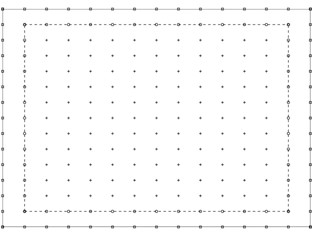
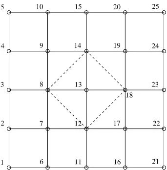
on a rectangular domain (xA≤x≤xB, yC≤y≤yD), and subject to Dirichlet bound-ary conditions (i.e. u and∂u/∂n given at the boundaries (n the normal direction)). The problem domain is represented by a Cartesian grid of nx×ny as shown in Figure 1. We employ fourth-order IRBF schemes for compact local 5×5-node and 13-node stencils, and second-order IRBF schemes for compact local 3×3-node stencils.

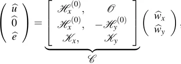
4.1 Compact local 5×5-node stencil (5×5-node CLS)

Consider a grid node (i,j) and its associated 5×5-node stencil. The stencil is locally numbered from left to right and from bottom to top (node (i,j)≡ node 13) (Figure 2). The solution procedure here is similar to that for 1D problems. However, the 2D problem formulation involves more terms and requires special treatments for interior “corner” nodes.

The conversion system is constructed as



 b

u

b0

b

e



=

  

H_x(0)_, O H_x(0)_{, −}H_y(0)

K_x, K_y

  

| {z }

C

b

wx

b

wy

, (35)

of zeros, respectively; equationsu_b=H_x(0)_{wbx are employed to collocate the} vari-able u over the stencil; equationsH_x(0)_{wxb −}H_y(0)_{wyb =}b_{0 are employed to enforce} nodal values of u obtained from the integration with respect to x and y to be identi-cal; and equationsK_{xwxb +}K_{ywyb =be are employed to represent extra information} that can be values of the PDE (20) at selected nodes on the stencil and first-order derivative boundary conditions. In (35), C _{is the conversion matrix, u andb} b_{0 are} vectors of length 25; (wx,b wyb )T _{is the RBF coefficient vector of length 90, and} O_,H_x(0)_,H_y(0)_,K_xandK_{yare matrices (the first three are of dimensions 25×45,} while for the last two, their dimensions are dependent on the number of extra infor-mation values imposed and typically vary between 4×45 to 6×45). Solving (35) yields

b

wx

b

wy

=C−1



 b

u

b

0

b

e



. (36)

We present two ways, namely Implementation 1 and Implementation 2, to form the final set of algebraic equations.

Implementation 1: The final system is composed of two sets of equations. The first set is obtained by collocating the PDE at interior nodes (i,j) with (3≤i≤ nx−2 and 3≤j≤ny−2) and the second set is obtained by imposing first derivative boundary conditions at boundary nodes (i=1,2≤ j≤ny−1), (i=nx,2≤ j≤ ny−1), (3≤i≤nx−2, j=1) and (3≤i≤nx−2, j=ny).

Implementation 2: First derivative boundary conditions are incorporated into the conversion system and the final system is formed by collocating the PDE only at all interior nodes.

Some implementation notes:

1. In constructing the approximations for stencils, the cross derivative∂4u/∂x2∂y2 is computed through the following relation [Mai-Duy and Tanner (2005a)], which requires the approximation of second-order pure derivatives only,

∂4_u

∂2x∂2_y=

1 2

_∂2

∂x2 _∂2

u ∂y2

+ ∂

2

∂y2 _∂2

u ∂x2

= 1

2

H_x(2)hH_x(0)i−1H_y(2)_wyb+H_y(2)hH_y(0)i−1H_x(2)_{wxb. (37)}

(i+1,j)) as shown in Figure 2. The extra information vector can thus be expressed in the form

   

f(x8)

f(x12)

f(x14)

f(x18)    =    

G_x(8,:),G_y(8,:) G_x(12,:),G_y(12,:) G_x(14,:),G_y(14,:) G_x(18,:),G_y(18,:)

    b wx b wy , (38) where

G_x=H_x(4)₊H_y(2)hH_y(0)i−1H_x(2)_,

and

G_y=H_y(4)₊H_x(2)hH_x(0)i−1H_y(2)_.

3. For stencils whose central points are (3,3), (3,ny−2), (nx−2,3) and (nx−2,ny− 2), the extra information vector is comprised of four nodal values of the derivative boundary condition and two nodal values of the PDE. For example, in the case of

(3,3), we formbe =K_{xwxb +}K_{ywyb as}

              

∂u(x2)

∂x ∂u(x3)

∂x ∂u(x6)

∂y ∂u(x11)

∂y f(x14)

f(x18)                =          

H_x(1)_(2,:), O H_x(1)_(3,:), O

O_, H_y(1)_(6,:) O_, H_y(1)_(11,:) Gx(14,:), Gy(14,:)

Gx(18,:), Gy(18,:)

          b wx b wy . (39)

4. For stencils whose central points are (i=3,3< j<ny−2), (i=nx−2,3<j< ny−2), (3<i<nx−2, j=3) and (3<i<nx−2, j=ny−2), the extra information vector is comprised of one nodal value of the derivative boundary condition and three nodal values of the PDE. For example, in the case of (i=3,3< j<ny−2), we form_be =K_xwbx+K_ywbyas

     

∂u(x3)

∂x f(x12)

f(x14)

f(x18)      =    

H_x(1)_(3,:), O Gx(12,:), Gy(12,:)

Gx(14,:), Gy(14,:)

Gx(18,:), Gy(18,:)

    b wx b wy . (40)

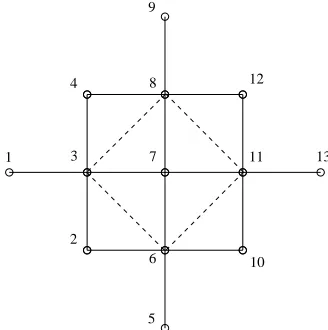
4.2 Compact local 13-node stencil (13-node CLS)

Figure 3 shows a schematic outline of a compact local 13-node stencil. The con-struction of the final system matrix using 13-node CLS is similar to that with 5 ×5-node CLS. Since the present stencil involves 13 ×5-nodes rather than 25 ×5-nodes, a sparse level (i.e. the number of zero entries) of the system matrix increases and its solution is thus more efficient. However, one can expect that 13-node CLS is less accurate than 5×5-node CLS.

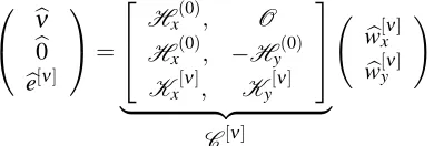
4.3 Compact local 3×3-node stencil (3×3-node CLS)

A 3×3-node CLS is constructed through a coupled set of two Poisson equations ∂2ν

∂x2 +

∂2ν

∂y2 =f(x,y), (41)

∂2_u

∂x2+

∂2_u

∂y2 =ν, (42)

which represent the biharmonic equation (34).

Consider a grid node(i,j)(2≤i≤nx−1,2≤j≤ny−1) and its associated 3× 3-node stencil



xx32 xx65 xx98

x1 x4 x7 

((i,j)≡x5).

4.3.1 Discretisation of equation (41)

Over a 3×3-node stencil, we construct the conversion system as

  bνb0

b

e[ν]



=

  

H_x(0)_, O H_x(0)_{, −}H_y(0) K_x[ν]_, K_y[ν]

  

| {z }

C[ν]

b

w[xν]

b

w[yν]

!

, (43)

where νb and b0 are vectors of length 9, (wbx[ν],wb[yν])T is the vector of length 30, H_x(0)_,H_y(0)_{are the matrices of dimensions 9×15, and equationsbe}[ν]₌K_x[ν]_wb[_xν]₊ K_y[ν]_wb[_yν]_{can be used to represent extra information. Like 3-node CLS for 1D} prob-lems, we study here two cases ofe_b[ν]. For the first case, the vector _be[ν] is used to represent nodal values of the governing equation at the four nodes x1, x3, x7 and

x9. Hereafter, this stencil is referred to as 3×3-node CLS with GE. For the second

A mapping from the physical space into the RBF-coefficient space is obtained by solving (43)

b

w[xν]

b

w[yν]

!

= (C[ν]₎−1

  b ν b 0 b

e[ν]



. (44)

Making use of (44), one can express the PDE (41) at the central point of the stencil as

h

H_x(2)_(5,:), H_y(2)_(5,:)

i

C[ν]−1

| {z }

D[ν]

  bνb0

b

e[ν]



= f(x5). (45)

It can reduce to D[ν]

1 bν+D [ν]

2 be[ν]= f(x5), (46)

whereD[ν]

1 andD [ν]

2 are the first 9 entries and the last 4 entries ofD[ν], respectively.

In (46),D[ν]

2 beν and f(x5)are known values.

4.3.2 Discretisation of equation (42)

Unlike equation (41), we consider nodal values of the field variable at grid nodes, ∂u/∂x at x2 and x8, and∂u/∂y at x4 and x6 as unknowns in the discretisation of

(42). The conversion matrix is thus formed as

     b u b0 c ∂ux c

∂uy

    =     

H_x(0)_, O H_x(0)_{, −}H_y(0) H_x(1)_([2,8],:), O

O_, H_y(1)_([4,6],:)

    

| {z }

C[u]

b

w[xu]

b

w[yu]

!

, (47)

where∂cux= (∂u(x2)/∂x,∂u(x8)/∂x)T and∂cuy= (∂u(x4)/∂y,∂u(x6)/∂y)T. It is

noted that the present additional unknowns∂cux and∂cuyare defined and located in the same way as in the FDM work [Stephenson (1984)].

Solving (47) results in

b

w[xu]

b

w[yu]

!

=C[u]−1

     b u b0 c

∂ux

c

∂uy

   

Equation (48) can be split into

b

w[xu]=

C_x[u]−1 _u,b b_0, ∂c_u x, ∂cuy

T

, (49)

b

w[yu]=

C_y[u]−1 _u,b b_0, ∂c_u x, ∂cuy

T

, (50)

where(C_x[u]₎−1_and(C_y[u]₎−1_{are the first and the last 15 rows of(}C[u]₎−1_.

Through (49) and (50), the first derivatives of u at the central point of the stencil can be computed by

∂u(x5)

∂x =H

(1)

x (5,:)

C_x[u]−1

     b u b0 c

∂ux

c ∂uy    

, (51)

∂u(x5)

∂y =H

(1)

y (5,:)

C_y[u]−1

     b u b0 c

∂ux

c ∂uy    

. (52)

Through (48), the discrete form of equation (42) over the stencil can be written as

h

H_x(2)_, H_y(2)

i

C[u]−1

| {z }

D[u]

     b u b 0 c ∂ux c ∂uy    

=νb. (53)

Substitution of (53) into (46) leads to a discrete form of the biharmonic equation (34) at the central point of the stencil

D[ν]

1 D[

u]      b u b0 c

∂ux

c ∂uy    

= f(x5)−D [ν]

2 bfk. (54)

By applying (51), (52) and (54) at every interior node, we will obtain the final system matrix of dimensions 3(nx−2)(ny−2)×3(nx−2)(ny−2).

5 Numerical examples

The accuracy of the solution is measured using the relative discrete L2norm

Ne(u) =

r _n

∑ i=1

(ui−uei)2

r _n

∑ i=1

(ue_i)2

, (55)

where n is the number of collocation nodes, and ui and uei are the computed and exact solutions, respectively.

We will study the behavior of the solution u with respect to (i) the grid size h, and (ii) the MQ widthβ.

5.1 One-dimensional problem

Consider the following fourth-order ODE

d4u dx4 +

d2u dx2 =16π

4_{sinh(2πx) +4π}2_{sinh(2πx), 0≤x≤2. (56)}

Double boundary conditions are defined as u=0 and du/dx=2π at x=0, and u=0 and du/dx=2πcosh(4π) at x=2. The exact solution to this problem can be verified to be ue(x) =sinh(2πx).

We employ 5-node CLS and 3-node CLS without and with GE to discretise (56). To assess the performance of the proposed stencils, the standard local 5-node IRBF stencil is also implemented. We conduct the calculations with several uniform grids,(7,9,· · ·,37).

Figure 4 displays the solution accuracy and the matrix condition numbers against the grid size h. In terms of accuracy (Figure 4a), the solution converges apparently as O(h1.40)for local 5-node stencil, and O(h5.45), O(h3.96)and O(h4.16)for 5-node CLS and 3-node CLS without and with GE, respectively. The compact forms, even for the case of 3-nodes, thus outperform the standard form of 5 nodes as indicated by not only the norm error but also the convergence rate. It can be also seen that 3-node CLS with GE is more accurate than that without GE. In terms of the matrix condition number (Figure 4b), the 5-node CLS and the standard 5-node stencil yield similar values. It can be also seen that the inclusion of first derivatives in the IRBF approximations, i.e 3-node CLSs, leads to higher condition numbers of the system matrix.

give similar levels of accuracy. However, Figure 5b shows that Implementation 2 yields better condition numbers than Implementation 1, probably owing to the fact that the final system matrix of the former is composed of equations derived from the ODE only.

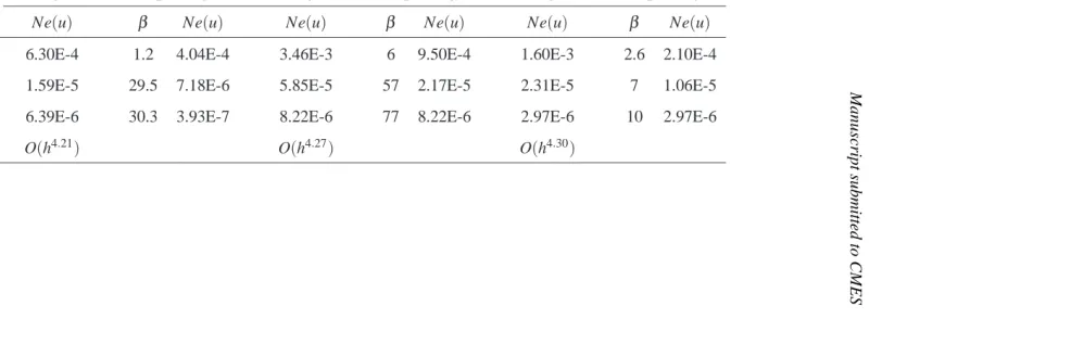
As mentioned earlier, the value ofβ would have a strong influence on the solution accuracy. Since the exact solution to this problem is available, it is straightforward to obtain the optimal value ofβ (i.e. at which Ne(u)is minimum). Table 1 shows results obtained by a fixed value and the optimal value ofβfor three different grids. It can be seen that using the optimal value ofβ significantly enhances the solution accuracy.

5.2 Two-dimensional problems 5.2.1 Example 1

Consider the biharmonic problem with the source function f(x,y) =64π4_sin(2πx_)sin(2πy_),

the domain of interest as 0≤x,y≤1 and boundary conditions of the Dirichlet type. The exact solution is ue(x,y) =sin(2πx)sin(2πy).

Figure 6 shows the behaviour of the solution u using the proposed 13-node CLS (β =18) with respect to the grid size h. Results obtained by the FD 13-node stencil are also included for comparison purposes. The IRBF method (Implementation 2) is much more accurate and converges much faster than the FDM (Figure 6a). The rate of convergence is 4.90 for the former and 1.99 for the latter. On the other hand, the IRBF matrix has higher condition numbers but grows slightly slower than the FD matrix (Figure 6b). The rate of growth is 3.25 for the former and 3.97 for the latter. Figure 7 indicates that Implementation 2 slightly outperforms Implementation 1 in terms of the matrix condition and accuracy. However, an improvement in the matrix condition here is not as significant as in the case of 1D problems.

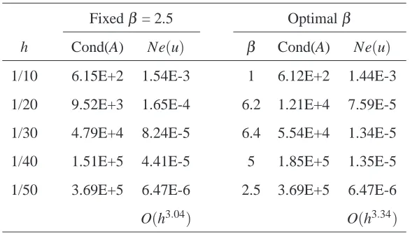
Table 2 presents results by the proposed 5×5-node CLS for a fixed value and the optimal value of β. It can be seen that the MQ width has more influence on the solution accuracy than on the system matrix condition number. It is noted that a chosen fixed valueβ =2.5 is the optimal value for the grid with h=1/50.

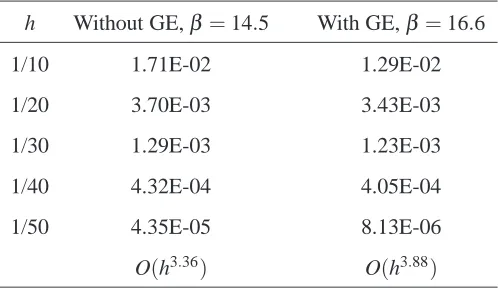
Table 3 shows the accuracy and matrix condition number against the grid size by the proposed 3×3-node CLS without and with GE. The solution converges as O(h3.36)

5.2.2 Example 2

Among our proposed compact stencils, the 3×3-node CLS does not require special treatments for interior nodes close to the boundary. This stencil is applied here to obtain the structure of the steady-state lid-driven cavity flow in the streamfunction-vorticity formulation

∂ψ ∂y

∂ω ∂x −

∂ψ ∂x

∂ω ∂y =

1 Re

_∂2_ω

∂x2 +

∂2_ω

∂y2

, (57)

−ω=∂

2ψ

∂x2 +

∂2ψ

∂y2 , (58)

where Re is the Reynolds number,ψ is the streamfunction andω is the vorticity. One can compute the x−and y−velocity components according to the following definitions

u=∂ψ

∂y and v=− ∂ψ

∂x.

The boundary conditions are prescribed in terms of the streamfunction as

ψ=0, ∂ψ

∂x =0 at x=0 and x=1, (59)

ψ=0, ∂ψ

∂y =0 at y=0, (60)

ψ=0, ∂ψ

∂y =1 at y=1. (61)

We employ several grids, (21×21,31×31,· · ·,111×111), in the simulation of the flow. A wide range of Re,(0,100,400,1000,3200,5000), is considered and the resultant nonlinear set of algebraic equations is solved using the Picard iteration scheme

b

θ=αθb(k)_{+ (1−α)θb}(k−1)_{, (62)}

where the superscript(k)is used to indicate the current iteration,α is the relaxation factor (0<α≤1)andθb= (ψb,d∂ψ

∂x,

d_∂ψ

∂y) T_.

The flow is considered to reach a steady state when

r

∑_θb(k)₋θb(k−1)2 r

∑_θb(k)2

As shown in Section 4.3, the proposed formulation does not require the derivation of a computational boundary condition for the vorticity and nodal values of the velocity components are obtained directly from solving the final system.

The value of β is chosen to be 20 for all simulations, while the value of α is employed in the range of 0.8 to 10−5. The higher the value of Re the smaller the value ofα will be.

The profile of the x−component of the velocity vector along the vertical centreline and of the y−component along the horizontal centreline for Re=1000 using sev-eral grids are demonstrated in Figure 8 and Figure 9, respectively. To provide the base for assessment, results obtained by the multi-grid FDM [Ghia, Ghia, and Shin (1982)], which are widely cited in the literature, are included. It can be seen that a convergence with grid refinement is obtained for both velocity profiles.

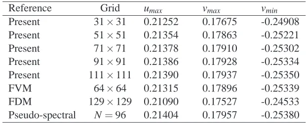
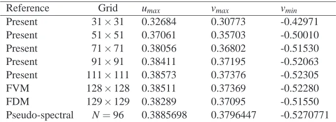
Tables 4 and 5 give a comparison of the extreme values of the velocity profile on the centrelines obtained by the proposed method, FDM [Ghia, Ghia, and Shin (1982)], FVM [Deng, Piquet, Queutey, and Visonneau (1994)] and the pseudo-spectral method [Botella and Peyret (1998)]. It can be seen that the present results are in better agreement with the benchmark spectral solution than the others even for ‘coarse’ grids, e.g. 51×51 in the case of Re=100 and 91×91 in the case of Re=1000.

Results concerning the distribution of of the streamfunction and vorticity over the flow domain are shown in Figures 10 and 11, respectively. They look feasible in comparison with those in literature (e.g. [Ghia, Ghia, and Shin (1982); Botella and Peyret (1998); Deng, Piquet, Queutey, and Visonneau (1994)]).

6 CONCLUDING REMARKS

Acknowledgement The first author would like to thank CESRC, FoES and USQ for a PhD scholarship. This research was supported by the Australian Research Council.

References

Altas, I.; Dym, J.; Gupta, M.; Manohar, R. (1998): Multigrid solution of auto-matically generated high-order discretizations for the biharmonic equation. SIAM Journal on Scientific Computing, vol. 19, pp. 1575–1585.

An-Vo, D.-A.; Mai-Duy, N.; Tran-Cong, T. (2011): A C2-continuous Control-Volume technique based on Cartesian grids and two-node integrated-RBF elements for second-order elliptic problems. Computer Modeling in Engineering & Sci-ences, vol. 72, pp. 299–334.

Bjørstad, P. (1983): Fast numerical solution of the biharmonic Dirichlet problem on rectangles. SIAM Journal on Numerical Analysis, vol. 20(1), pp. 59–71.

Botella, O.; Peyret, R. (1998): Benchmark spectral results on the Lid-driven cavity flow. Computers & Fluids, vol. 27, pp. 421–433.

Conte, S.; Dames, R. (1958): An alternating direction method for solving the biharmonic equation. Mathematical Tables and Other Aids to Computation, vol. 12 (63), pp. 198–205.

Deng, G.; Piquet, J.; Queutey, P.; Visonneau, M. (1994): Incompressible flow calculations with a consistent physical interpolation finite volume approach. Computers & Fluids, vol. 23, pp. 1029–1047.

Franke, R. (1982): Scattered data interpolation: Tests of some methods. Mathe-matics of Computation, vol. 38 (157).

Ghia, U.; Ghia, K.; Shin, C. (1982): High-Re solutions for Incompressible flow using the Navier-Stokes equations and a multigrid method. Journal of Computa-tional Physics, vol. 48, pp. 387–411.

Gupta, M.; Manohar, R. (1979): Direct solution of the bihramonic equations using noncoupled approach. Journal of Computational Physics, vol. 33, pp. 236– 248.

Hughes, T. (1987): The Finite Element Method: Linear Static and Dynamic Finite Element Analysis. Prentice-Hall.

Kansa, E. (1990): Multiquadrics - A scattered data approximation scheme with applications to computational fluid-dynamics - I Surface approximations and partial derivative estimates. Computers & Mathematics with Applications, vol. 19(8-9), pp. 127–145.

Kansa, E. (1990): Multiquadrics - A scattered data approximation scheme with applications to computational fluid-dynamics - II Solutions to parabolic, hyperbolic and elliptic partial differential equations. Computers & Mathematics with Appli-cations, vol. 19(8-9), pp. 147–161.

Kansa, E. (1999): Motivation for using radial basis functions to solve PDEs. Mathematical Modelling and Industrial Mathematics Papers, vol. 94551, pp. 1–8. Mai-Duy, N. (2005): Solving high order ordinary differential equations with radial basis function networks. International Journal for Numerical Methods in Engineering, vol. 62(6), pp. 824–852.

Mai-Duy, N.; Tanner, R. (2005): Computing non-Newtonian fluid flow with radial basis function networks. International Journal for Numerical Methods in Fluids, vol. 48(12), pp. 1309–1336.

Mai-Duy, N.; Tanner, R. (2005): Solving high-order partial differential equations with indirect radial basis function networks. International Journal for Numerical Methods in Engineering, vol. 63(11), pp. 1636–1654.

Mai-Duy, N.; Tran-Cong, T. (2001): Numerical solution of differential equations using multiquadric radial basis function networks. Neural Networks, vol. 14, pp. 185–199.

Mai-Duy, N.; Tran-Cong, T. (2003): Approximation of function and its deriva-tives using radial basis function networks. Applied mathematical modeling, vol. 27, pp. 197–220.

Mai-Duy, N.; Tran-Cong, T. (2009): A Cartesian-grid discretisation scheme based on local integrated RBFNs for two-dimensional elliptic problems. Computer Modeling in Engineering and Sciences, vol. 51(3), pp. 213–238.

Mai-Duy, N.; Tran-Cong, T. (2011): Compact local integrated-RBF approxi-mations for second-order elliptic differential problems. Journal of Computational Physics, vol. 230, pp. 4772–4794.

Ngo-Cong, D.; Mai-Duy, N.; Karunasena, W.; Tran-Cong, T. (2010): Free vibration analysis of laminated composite plates based on FSDT using one-dimensional IRBFN method. Computers and Structures, vol. 89(1-2), pp. 1–13.

Patankar, S. (1980): Numerical Heat Transfer and Fluid Flow. McGraw-Hill, New York.

Rannacher, R. (1999): Finite Element methods for the incompressible Navier-Stokes equations, 1999.

Reddy, J. (2005): An introduction to the finite element method (Third Edition). McGraw-Hill.

Smith, G. (1978): Numerical solution of partial differential equations: finite difference methods. Oxford: Clarendon Press.

M

a

n

u

sc

ri

p

t

su

b

m

itt

ed

to

C

M

E

S

5-node CLS 3-node CLS

Without GE With GE

h Fixedβ=24 Optimalβ Fixedβ=77 Optimalβ Fixedβ=10 Optimalβ

Ne(u) β Ne(u) Ne(u) β Ne(u) Ne(u) β Ne(u)

1/20 6.30E-4 1.2 4.04E-4 3.46E-3 6 9.50E-4 1.60E-3 2.6 2.10E-4

1/50 1.59E-5 29.5 7.18E-6 5.85E-5 57 2.17E-5 2.31E-5 7 1.06E-5

1/70 6.39E-6 30.3 3.93E-7 8.22E-6 77 8.22E-6 2.97E-6 10 2.97E-6

Table 2: PDE, Example 1, 5×5-node CLS: Condition numbers of the system ma-trix A and relative L2 errors of the solution u using a fixed value and the optimal

value ofβ for several grids.

Fixedβ = 2.5 Optimalβ

h Cond(A) Ne(u) β Cond(A) Ne(u)

1/10 6.15E+2 1.54E-3 1 6.12E+2 1.44E-3

1/20 9.52E+3 1.65E-4 6.2 1.21E+4 7.59E-5 1/30 4.79E+4 8.24E-5 6.4 5.54E+4 1.34E-5

1/40 1.51E+5 4.41E-5 5 1.85E+5 1.35E-5

Table 3: PDE, Example 1, 3×3-node CLS: relative L2errors of the solution u for

several grids.

h Without GE,β =14.5 With GE,β =16.6

1/10 1.71E-02 1.29E-02

1/20 3.70E-03 3.43E-03

1/30 1.29E-03 1.23E-03

1/40 4.32E-04 4.05E-04

1/50 4.35E-05 8.13E-06

Table 4: PDE, Example 2, Re=100, β =20: Extreme values of the velocity profiles on the centerlines by the proposed method and several other methods. It is noted that N is the polynomial degree.

Reference Grid umax vmax vmin

Present 31×31 0.21252 0.17675 -0.24908

Present 51×51 0.21354 0.17863 -0.25221

Present 71×71 0.21378 0.17910 -0.25302

Present 91×91 0.21386 0.17928 -0.25334

Present 111×111 0.21390 0.17937 -0.25350

FVM 64×64 0.21315 0.17896 -0.25339

FDM 129×129 0.21090 0.17527 -0.24533

Table 5: PDE, Example 2, Re=1000, β =20: Extreme values of the velocity profiles on the centerlines by the proposed method and several other methods. It is noted that N is the polynomial degree.

Reference Grid umax vmax vmin

Present 31×31 0.32684 0.30773 -0.42971

Present 51×51 0.37061 0.35703 -0.50010

Present 71×71 0.38056 0.36802 -0.51530

Present 91×91 0.38411 0.37195 -0.52063

Present 111×111 0.38573 0.37376 -0.52305

FVM 128×128 0.38511 0.37369 -0.52280

FDM 129×129 0.38289 0.37095 -0.51550

2

1 3 4 5

6 7 8 9 10

11 12 13 14 15

16 17 19 20

21 23

22 24 25

18

2 4

5 6 8 9

10 12

11 13

1 3 7

10−1 10−5

10−4 10−3 10−2 10−1 100

Standard local IRBF 5−node

5−node CLS

3−node CLS without GE

3−node CLS with GE

Grid spacing

N

e

(

u

)

(a)

10−1 100

102 104 106 108 1010

Standard local IRBF 5−node 5−node CLS

3−node CLS without GE 3−node CLS with GE

Grid spacing

C

o

n

d

it

io

n

n

u

m

b

er

(b)

Figure 4: ODE: Relative L2 errors of the solution u and condition numbers of the

10−1 10−5

10−4 10−3 10−2 10−1 100

Implementation 1

Implementation 2

Grid spacing

N

e

(

u

)

(a)

10−1 101

102 103 104 105 106 107 108

Implementation 1

Implementation 2

Grid spacing

C

o

n

d

it

io

n

n

u

m

b

er

(b)

10−1 10−5

10−4 10−3 10−2 10−1 100

FD 13−node

13−node CLS

Grid spacing

N

e

(

u

)

(a)

10−1 102

104 106 108 1010 1012

FD 13−node

13−node CLS

Grid spacing

C

o

n

d

it

io

n

n

u

m

b

er

(b)

10−1 10−5

10−4 10−3 10−2 10−1 100

Implementation 1

Implementation 2

Grid spacing

N

e

(

u

)

(a)

10−1 107

108 109 1010 1011

Implementation 1

Implementation 2

Grid spacing

C

o

n

d

it

io

n

n

u

m

b

er

(b)

−0.40 −0.2 0 0.2 0.4 0.6 0.8 1 0.1

0.2 0.3 0.4 0.5 0.6 0.7 0.8 0.9 1

Ghia et al Present 31×31 Present 91×91 Present 111×111

u

y

0 0.1 0.2 0.3 0.4 0.5 0.6 0.7 0.8 0.9 1 −0.6

−0.5 −0.4 −0.3 −0.2 −0.1 0 0.1 0.2 0.3 0.4

Ghia et al

Present 31×31

Present 91×91

Present 111×111

x

v

0 0.2 0.4 0.6 0.8 1 0 0.1 0.2 0.3 0.4 0.5 0.6 0.7 0.8 0.9

1 Re=0

0 0.2 0.4 0.6 0.8 1

0 0.1 0.2 0.3 0.4 0.5 0.6 0.7 0.8 0.9

1 Re=100

0 0.2 0.4 0.6 0.8 1

0 0.1 0.2 0.3 0.4 0.5 0.6 0.7 0.8 0.9

1 Re=400

0 0.2 0.4 0.6 0.8 1

0 0.1 0.2 0.3 0.4 0.5 0.6 0.7 0.8 0.9

1 Re=1000

0 0.2 0.4 0.6 0.8 1

0 0.1 0.2 0.3 0.4 0.5 0.6 0.7 0.8 0.9

1 Re=3200

0 0.2 0.4 0.6 0.8 1

0 0.1 0.2 0.3 0.4 0.5 0.6 0.7 0.8 0.9

1 Re=5000

0 0.2 0.4 0.6 0.8 1 0 0.1 0.2 0.3 0.4 0.5 0.6 0.7 0.8 0.9

1 Re=0

0 0.2 0.4 0.6 0.8 1

0 0.1 0.2 0.3 0.4 0.5 0.6 0.7 0.8 0.9

1 Re=100

0 0.2 0.4 0.6 0.8 1

0 0.1 0.2 0.3 0.4 0.5 0.6 0.7 0.8 0.9

1 Re=400

0 0.2 0.4 0.6 0.8 1

0 0.1 0.2 0.3 0.4 0.5 0.6 0.7 0.8 0.9

1 Re=1000

0 0.2 0.4 0.6 0.8 1

0 0.1 0.2 0.3 0.4 0.5 0.6 0.7 0.8 0.9

1 Re=3200

0 0.2 0.4 0.6 0.8 1

0 0.1 0.2 0.3 0.4 0.5 0.6 0.7 0.8 0.9

1 Re=5000