Galerkin/collocation methods based on 1D-integrated-RBFNs for viscoelastic flows

flows

D. Ho-Minh1, N. Mai-Duy1and T. Tran-Cong1

Abstract: In this paper, one-dimensional integrated radial-basis-function networks (1D-IRBFNs) are intro-duced into the Galerkin and point-collocation formulations to simulate viscoelastic flows. The computational domain is represented by a Cartesian grid and IRBFNs, which are constructed through integration, are em-ployed on each grid line to approximate the field variables including stresses in the streamfunction-vorticity formulation. Two types of fluid, namely Oldroyd-B and CEF models, are considered. The proposed meth-ods are validated through the numerical simulation of several benchmark test problems including flows in a rectangular duct and in a corrugated tube. Numerical results show that accurate results are obtained using relatively-coarse grids.

Keywords: viscoelastic flows, Cartesian grid, 1D integrated RBFNs, point collocation, Galerkin formulation.

1 Introduction

Numerical simulation of viscoelastic flows still faces a lot of challenges. Main difficulties, which numerical methods have to deal with, are (i) complex material properties of fluids, (ii) mixed characters (elliptic for momentum equations and hyperbolic for constitutive equations), and (iii) high degrees of freedom (DOF) (2D problems: 6 DOFs/node and 3D problems: 10 DOFs/node). In the case of large deformations, free/moving surfaces and complex geometries, further numerical difficulties will be added. One can classify discretisation methods into two categories: low order and high order. The former, e.g. traditional finite difference (FDMs), finite element (FEMs), finite volume (FVMs) and boundary element (BEMs) methods, leads to a system matrix that is generally sparse and banded (possibly block-banded BEM), while the latter, e.g. spectral and RBFN methods, can offer a significant saving on the computational cost owing to their high-order rates of convergence. Further details can be found in [Crochet and Walters (1983); Crochet, Davies, and Walters (1984); Crochet (1989); Tanner and Xue (2002); Owens and Phillips (2002)].

The use of RBFNs for solving ordinary (ODEs) and partial (PDEs) differential equations has been an active research area since Kansa’s first report in 1990 [Kansa (1990)]. For Kansa’s method (direct approach), the field variable f in the ODE/PDE is first represented by an RBFN and this RBFN is then differentiated to obtain approximate expressions for derivative functions of f (differentiated RBFNs (DRBFN)). On the other hand,

in order to avoid the reduction in convergence rate caused by differentiation, Mai-Duy and Tran-Cong (2001) proposed an indirect approach in which the highest-order derivatives of f are first decomposed into RBFs, and their lower-order derivatives and the function f itself are then obtained through integration (integrated RBFN (IRBFN)). Numerical experiments (e.g. [Mai-Duy and Tran-Cong (2001, 2003)]) showed that IRBFN collocation methods yield better accuracy than DRBFN ones for both the representation of functions and the solution of PDEs. In the early stages, both direct and indirect approaches used every RBF to construct the approximations for the field variable at a nodal point, leading to a fully-populated system matrix. It was found that the matrix condition number grows rapidly with respect to the increase in the RBF width and/or the number of RBFs [Schaback (1995)]. Global RBF solutions to steady viscoelastic flows were reported in, e.g., [Tran-Cong, Mai-Duy, and Phan-Thien (2002); Tran-Canh and Tran-Cong (2002); Mai-Duy and Tanner (2006)]. Later on, local RBF techniques, where the approximations are constructed using only a few nodal points, have been developed (e.g. [Atluri, Han, and Shen (2003); Atluri, Han, and Rajendran (2004); Sˇarler (2005); Mai-Duy and Tran-Cong (2009); Sellountos, Sequeira, and Polyzos (2010)]). In the context of IRBFNs, collocation schemes, based on 1D-IRBFNs and Cartesian grids, for the solution of 2D elliptic PDEs were reported in, e.g., [Mai-Duy and Tran-Cong (2007)]. The 1D-IRBFN approximations at a grid node involve only nodal points that lie on the grid lines intersecting at that point rather than the whole set of nodes. As a result, the construction process is conducted for a series of small matrices rather than for a large single matrix (thus some degree of local approximation is achieved).

1D-IRBFNs were successfully introduced into the point-collocation and Galerkin formulations for the simula-tion of heat transfer and Newtonian-fluid flows (e.g. [Mai-Duy and Tran-Cong (2007); Mai-Duy, Ho-Minh, and Tran-Cong (2009); Ho-Minh, Mai-Duy, and Tran-Cong (2009)]). It was shown that those methods are stable, accurate and converge well. The 1D-IRBFN-based Galerkin method can obtain similar levels of accuracy for both types of boundary condition, i.e. Dirichlet only and Dirichlet-Neumann. In addition, its resultant sys-tem of algebraic equations is often symmetric and has a relatively-low condition number, which facilitates the employment of a much larger number of nodes.

The remainder of this paper is organised as follows. In Section 2, a brief review of the governing equa-tions for the motion of CEF and Oldroyd-B fluids is given. Section 3 presents the proposed 1D-IRBFN-based Galerkin/collocation methods. Three test problems are simulated in Section 4. Section 5 concludes the paper.

2 Governing equations

The equations for the conservation of momentum and mass of an incompressible fluid take the forms

ρ∂_∂v

t +v·∇v

= ∇·σ+f, x∈Ω, (1)

∇·v = 0, x∈Ω, (2)

where v is the velocity vector, f the body force vector per unit volume,ρthe density,σthe Cauchy stress tensor,

t the time, x the position vector andΩthe domain of interest. The stress tensor can be decomposed into

σ=−pI+τ, (3)

where p is the pressure, I the unit tensor andτ the extra stress tensor. In this paper, the working fluids are of the CEF and Oldroyd-B types.

For the CEF model, the extra stress tensor is defined as

τ=2µ(d)d−Φ1∇d+4Φ2d·d, (4)

where d=1/2(∇v+ (∇v)T) is the rate of deformation tensor, d=p2tr(d·d)the scalar magnitude of d (tr the trace operation), µ(d) =k|d|n−1_{the viscosity (k the consistency factor and n the power law index),}Φ1_and Φ2the first and the second normal stress coefficients, respectively, and[ ]∇ the upper convected derivative given by

∇ [ ] = ∂[ ]

∂t +v·∇[ ]−(∇v)

T_{·[ ]−[ ]·∇v.}

(5)

For the Oldroyld-B model, the extra stress tensor is computed as

τ = 2µnd+τv, (6)

τv+λ

∇

τv = 2µpd, (7)

whereµnis the “Newtonian-contribution” viscosity,µpthe “polymer-contribution” viscosity,τvthe extra stress

In this study, we consider the steady state of flows only and adopt the streamfunction-vorticity formulation. Eq. 1 - Eq. 3 thus reduce to

∇2_{ψ+ω = 0, (8)}

∇2_{ω = F(v·∇ω,τ,f), (9)}

whereψ is the streamfunction, ω the vorticity, and the RHS of Eq. 9 the function of v,ω,τ and f. Numerical examples to be presented are solved in two coordinate systems, namely Cartesian and cylindrical.

The velocity components are related to the streamfunction via

ux = −∂ψ_∂

y, uy=

∂ψ

∂x (Cartesian coordinates), (10)

ur = −

1

r

∂ψ

∂z , uz=

1

r

∂ψ

∂r (cylindrical coordinates). (11)

For the CEF model, simulations are to be carried out using Cartesian coordinates and Eq. 4 is taken in the form

Txx=2µdxx−Φ1

ux

∂dxx

∂x +uy

∂dxx

∂y +

∂ux

∂xdxx+

∂uy

∂x dxy+

∂uz

∂xdxz+dxx

∂ux

∂x +dxy∂

uy

∂x +dxz

∂uz

∂x

+ (Φ1+4Φ2) d_xx2 +d_xy2 +d_xz2, (12)

Txy=2µdxy−Φ1

ux∂

dxy

∂x +uy

∂dxy

∂y +

∂ux

∂xdxy+

∂uy

∂xdyy+

∂uz

∂xdyz+dxx

∂ux

∂y +dxy∂

uy

∂y +dxz

∂uz

∂y

+ (Φ1+4Φ2) (dxxdxy+dxydyy+dxzdyz), (13)

Txz=2µdxz−Φ1

ux∂

dxz

∂x +uy

∂dxz

∂y +

∂ux

∂xdxz+

∂uy

∂xdyz+

∂uz

∂xdzz+dxx

∂ux

∂z +dxy∂

uy

∂z +dxz

∂uz

∂z

+ (Φ1+4Φ2) (dxxdxz+dxydyz+dxzdzz), (14)

Tyy=2µdyy−Φ1

ux∂

dyz

∂x +uy

∂dyz

∂y +

∂ux

∂ydyx+

∂uy

∂ydyy+

∂uz

∂ydyz+dxy

∂ux

∂y +dyy∂

uy

∂y +dyz

∂uz

∂y

+ (Φ1+4Φ2) d_yx2 +d_yy2 +d_yz2, (15)

Tyz=2µdyz−Φ1

ux

∂dyz

∂x +uy

∂dyz

∂y +

∂ux

∂ydxz+

∂uy

∂ydyz+

∂uz

∂ydzz+dxy

∂ux

∂y +dyy

∂uy

∂y +dyz

∂uz

∂y

where

µ =k 2 ∂ux ∂x 2 + _∂ uy ∂y 2! + _∂ ux

∂y +

∂uy

∂x 2 + _∂ uz ∂x 2 + _∂ uz ∂y

2!(n−1 2 )

, (17)

and

 

dxx dxy dxz

dyx dyy dyz

dzx dzy dzz

 =     

∂ux

∂x

1 2

_∂

ux

∂y +

∂uy

∂x 1 2 _∂ ux

∂z +

∂uz

∂x 1 2 _∂u y

∂x +

∂ux

∂y _∂u y ∂y 1 2 _∂u y

∂z +

∂uz

∂y 1 2 _∂ uz

∂x +

∂ux

∂z 1 2 _∂ uz

∂y +

∂uy

∂z _∂ uz ∂z    

. (18)

The Oldroyd-B fluid flow is simulated using cylindrical coordinates and one thus has Eq. 7 in the form

Trr+λ

ur∂

Trr

∂r +uz

∂Trr

∂z −2

_∂

ur

∂r Trr+

∂ur

∂z Trz

=2µp∂

ur

∂r , (19)

Trz+λ

ur∂

Trz

∂r +uz

∂Trz

∂z −

∂ur

∂r Trz−

∂ur

∂z Tzz−

∂uz

∂r Trr−

∂uz

∂z Trz

=µp

_∂

ur

∂z +

∂uz

∂r

, (20)

Tzz+λ

ur∂

Tzz

∂r +uz

∂Tzz

∂z −2

_∂

uz

∂r Trz+

∂uz

∂z Tzz

=2µp∂

uz

∂z , (21)

T_θθ+λ

ur

∂Tθθ ∂r +uz

∂Tθθ ∂z −2

ur

r Tθθ

=2µp

ur

r . (22)

3 Proposed 1D-IRBFN-based Galerkin/Collocation techniques

The computational domain is simply represented by a Cartesian grid. On each grid line, 1D-IRBFNs are employed to approximate the field variables, i.e.ψ,ω, Txx, Txy, Tyy, Txz, Tyz, Trr, Trz, Tzzand Tθθ. The governing

equations Eq. 8 - Eq. 9, Eq. 12 - Eq. 16 and Eq. 19 - Eq. 22 are discretised by means of point collocation (the residual set to zero at the collocation points) or Galerkin formulation (the residual set to zero in the mean). In the following, details are presented for three main parts of the proposed methods. In the first part, the use of 1D-IRBFNs to represent the field variables is discussed. In the second part, the implementation of boundary conditions is described. In the third part, 1D-IRBFs are incorporated into the Galerkin and point-collocation formulations as the trial functions.

3.1 One-dimensional IRBFN representation of the field variables

It can be seen that Eq. 8 - Eq. 9 involve second-order derivatives of the field variables including stresses. As a result, the second-order integral RBF scheme [Mai-Duy and Tran-Cong (2003)] is applied in this work. Processes of constructing the 1D-IRBFN approximations for the field variables can be conducted in a similar fashion. For brevity, we introduce the notation f to representψ,ω, Txx, Txy, Tyy, Txz, Tyz, Trr, Trz, Tzzor Tθθ, and

On aη grid line, the field variable f and its derivatives with respect toη can be represented as follows.

d2_f(η₎

dη2 =

Nη

∑

i=1

wigi(η) = Nη

∑

i=1

wiIi(2)(η), (23)

d f(η)

dη =

Nη

∑

i=1

wiIi(1)(η) +c1, (24)

f(η) =

Nη

∑

i=1

wiIi(0)(η) +c1η+c2, (25)

where N_ηis the number of nodes on the grid line,{wi} Nη

i=1the set of network weights,{gi(η)} Nη i=1≡

n

I_i(2)(η)oNη

i=1 the set of RBFs, I_i(1)(η) =RI_i(2)(η)dη,I_i(0)(η) =RI_i(1)(η)dη, and c1and c2are the constants of integration. Evaluation of Eq. 23 - Eq. 25 at every node on the grid line leads to

d

d2_f

dη2 = Ib

(2)_{αb, (26)}

dd f

dη = Ib

(1)_{αb, (27)}

b

f = Ib(0)α_{b, (28)}

where the superscript(.)is used to denote the order of the corresponding derivative function,

b

I(2) ₌

      

I₁(2)(η1), I₂(2)(η1), · · ·, I_N(2_η)(η1), 0, 0

I₁(2)(η2), I₂(2)(η2), · · ·, I_N(2_η)(η2), 0, 0 ..

. ... . .. ... ... ...

I₁(2) ηNη

, I₂(2) ηNη

, · · ·, I_N(2_η) ηNη

b

I(1) ₌

      

I₁(1)(η1), I₂(1)(η1), · · ·, I_N(1_η)(η1), 1, 0

I₁(1)(η2), I₂(1)(η2), · · ·, I_N(1_η)(η2), 1, 0 ..

. ... . .. ... ... ...

I₁(1) ηNη

, I₂(1) ηNη

, · · ·, I_N(1_η) ηNη

, 1, 0        , b

I(0) ₌

      

I₁(0)(η1), I₂(0)(η1), · · ·, I_N(0_η)(η1), η1, 1

I₁(0)(η2), I₂(0)(η2), · · ·, I_N(0_η)(η2), η2, 1 ..

. ... . .. ... ... ...

I₁(0) ηNη

, I₂(0) ηNη

, · · ·, I_N(0_η) ηNη

, ηNη, 1

       , b

α = w1,w2,· · ·,wNη,c1,c2 T

,

and

d

dk_f

dηk =

dkf1

dηk,

dkf2

dηk,· · ·,

dkfNη dηk

!T

, k={1,2},

b

f = f1,f2,· · ·,fNη

T

,

in which dkfj

dηk=dkf(ηj)

dηkand fj= f(ηj)with j={1,2,· · ·,Nη}.

The relations between the RBF-coefficient spaceαb and the physical space bf can be established as

_b f b e = " b

I(0)

c

K

# b

α =Cbα_{b, (29)}

b

α = Cb−1

_b f b e , (30)

where _be=Kcα_{b is used to represent extra information (derivative data), which would otherwise be wasted}

resulting in less accurate solutions, andCb_{the conversion matrix. In Eq. 29 - Eq. 30, owing to the presence}

of the two integration constants, the vector_be can have up to two entries. Since the conversion matrixCb_{is not}

over-determined, extra values eiare incorporated into the IRBFN approximations in an exact manner. We will

utilise this capability to impose normal derivative values at the two end-points of the grid line as well as to derive a computational boundary condition for the vorticity.

by

f(η) = I₁(0)(η),I₂(0)(η),· · ·,I_N(0_η)(η),η,1Cb−1

_b f b e , (31)

∂f(η)

∂η =

I₁(1)(η),I₂(1)(η),· · ·,I_N(1_η)(η),1,0Cb−1

_b f b e , (32)

∂2_f(η) ∂η2 =

I₁(2)(η),I₂(2)(η),· · ·,I_N(2_η)(η),0,0Cb−1

_b f b e . (33)

They can be rewritten in compact form

f(η) =

Nη

∑

i=1

ϕi(η)fi+ϕNη+1(η)e1+ϕNη+2(η)e2, (34) ∂f(η)

∂η =

Nη

∑

i=1

∂ϕi(η)

∂η fi+

∂ϕNη+1(η) ∂η e1+

∂ϕNη+2(η)

∂η e2, (35)

∂2_f(η) ∂η2 =

Nη

∑

i=1 ∂2_ϕ

i(η)

∂η2 fi+ ∂2ϕ

Nη+1(η) ∂η2 e1+

∂2ϕ

Nη+2(η)

∂η2 e2, (36)

where{ϕi} Nη+2

i=1 is the set of IRBFN basis functions in the physical space.

3.2 Imposition of boundary conditions

Dirichlet boundary conditions: Assume that f is given atη1 and ηNη. In the conversion process, Eq. 29

-Eq. 30, the matrixKc_{and the vectorbe are simply set to null. The 1D-IRBFN expressions Eq. 34 - Eq. 36 thus}

reduce to

f(η) =

Nη

∑

i=1

ϕi(η)fi, (37)

∂f(η)

∂η =

Nη

∑

i=1

∂ϕi(η)

∂η fi, (38)

∂2_f(η) ∂η2 =

Nη

∑

i=1 ∂2_ϕ

i(η)

Neumann boundary conditions: Assume that∂f/∂ηis given atη1andηNη. The matrixKcand the vectorbe

in Eq. 29 - Eq. 30 take the form

c

K ₌

"

I₁(1)(η1), I₂(1)(η1), · · ·, I_N(1_η)(η1), 1, 0

I₁(1) ηNη

, I₂(1) ηNη

, · · ·, I_N(1_η) ηNη

, 1, 0 #

,

b

e =

∂f1

∂η ∂fN_η

∂η !

.

The 1D-IRBFN expressions Eq. 34 - Eq. 36 thus become

f(η) =

Nη

∑

i=1

ϕi(η)fi+ϕNη+1(η)∂

f1

∂η +ϕNη+2(η) ∂fNη

∂η , (40)

∂f(η)

∂η =

Nη

∑

i=1

∂ϕi(η)

∂η fi+

∂ϕNη+1(η) ∂η

∂f1 ∂η +

∂ϕNη+2(η) ∂η

∂fNη

∂η , (41)

∂2_f(η₎ ∂η2 =

Nη

∑

i=1 ∂2ϕ

i(η)

∂η2 fi+ ∂2_ϕ

Nη+1(η) ∂η2

∂f1 ∂η +

∂2_ϕ

Nη+2(η) ∂η2

∂fNη

∂η . (42)

Dirichlet and Neumann boundary conditions: Assume that f and∂f/∂η are given atη1andηNη,

respec-tively. The latter is imposed by taking the matrixKc_{and the vectorbe in Eq. 29 - Eq. 30 as}

c

K ₌ h _I(1)

1 ηNη

, I₂(1) ηNη

, · · ·, I_N(1_η) ηNη

, 1, 0 i

,

b

e = ∂fN_η

∂η

.

One thus has Eq. 34 - Eq. 36 in the form

f(η) =

Nη

∑

i=1

ϕi(η)fi+ϕNη+1(η) ∂fNη

∂η , (43)

∂f(η)

∂η =

Nη

∑

i=1

∂ϕi(η)

∂η fi+

∂ϕNη+1(η) ∂η

∂fNη

∂η , (44)

∂2_f(η₎ ∂η2 =

Nη

∑

i=1 ∂2ϕ

i(η)

∂η2 fi+ ∂2_ϕ

Nη+1(η) ∂η2

∂fNη

∂η . (45)

3.3 Incorporating 1D-IRBFNs into Galerkin and point-collocation formulations

Each governing equation in Eq. 8 - Eq. 9, Eq. 12 - Eq. 16 and Eq. 19 - Eq. 22 can be rewritten in the following form

whereL _{is a differential operator. 1D-IRBFN expressions Eq. 34 - Eq. 36 are utilised here to construct the}

approximations for f overΩ. On a 2D rectangular domain, this construction process can simply be done by means of Kronecker products. The use of tensor products leads to, for instance,

f(x,y) =

Nx

∑

i=1

Ny

∑

j=1 ϕ(x)

i (x)ϕ

(y)

j (y)fi,j, (47)

for the case of Dirichlet boundary conditions only, and

f(x,y) =

Nx

∑

i=1 ϕ(x)

i (x)

Ny

∑

j=1 ϕ(y)

j (y)fi,j+ϕN(yy+)1(y) ∂fi,1

∂y +ϕ (y)

Ny+2(y) ∂fi,Ny

∂y

!

. (48)

for the case of Dirichlet and Neumann boundary conditions (Dirichlet conditions prescribed on the two ver-tical boundaries while Neumann conditions on the two horizontal boundaries). In Eq. 47 and Eq. 48, fi,j is

the value of the variable f at the intersection of the ith horizontal grid line and jth vertical grid line, and ∂fi,1∂y and∂fi,Ny

∂y are nodal boundary derivative values. The products ϕ_i(x)ϕ(_jy)are usually referred to as the trial/basis/approximating functions.

It is noted that the independent variables x and y in Eq. 47 - Eq. 48 will be replaced with r and z if cylindrical coordinates are employed.

One can find the unknown nodal values of f by constructing a scheme to minimise the following residual

R=L(f). (49)

This process can be stated mathematically as

Z

ΩW RdΩ=0, (50)

where W is the weighting function to be chosen. In the point-collocation approach, the weighting function is chosen as the Dirac delta function, i.e. Wi =δ(x−xi). In the Galerkin approach, the weighting function is

chosen from the set of trial functions, i.e. Wi=φi(x), and the volume integrals in Eq. 50 can be numerically

evaluated using Gauss quadrature.

As mentioned earlier, Neumann boundary conditions are presently imposed in an exact manner. This is numer-ically demonstrated here through the solution of the following ODE

d2f

dx2 +f+x=0, 0≤x≤1, (51)

subject to a Dirichlet and Neumann boundary condition at x=0 and x=1, respectively.

statement 1 Z 0 d f dx dW

dx −(f+x)W

dx= [qW]_x=1, (52)

which is obtained by applying integration by parts on Eq. 50. As shown in [Brebbia, Telles, and Wrobel (1984)], by differentiating the approximate function f , one has

d f dx

x=1

=1.22E-1+ (1+1.22E-1)q,

which clearly indicates that the Neumann boundary condition is imposed in an approximate manner.

In the present Galerkin technique, the IRBFN approximation is constructed to satisfy not only the Dirichlet condition at x=0 but also the Neumann boundary condition d f/dx=q at x=1. Using Eq. 43, the solution f is expressed as

f(x) =

∑

i=1ϕi(x)fi+ϕNx+1(x)q¯. (53)

This approximation is then forced to satisfy the ODE through

Z 1

0

d2f

dx +f+x

W dx=0, (54)

from which one is able to obtain the nodal values of f . By differentiating Eq. 53, one has

d f dx

x=1

=

∑

i=1

dϕi(x=1)

dx fi+

dϕNx+1(x=1)

dx q¯.

With Nx=5, it reduces to

d f dx

x=1

= (-1.87E-14) + (1+5.07E-14)q≃q,

which clearly shows that the Neumann boundary condition is imposed in an exact manner.

4 Numerical results

The proposed methods are validated through the simulation of viscoelastic flows in rectangular ducts (with Galerkin formulation), and in straight and corrugated tubes (point collocation). Fluid models under considera-tion here are CEF and Oldroyd-B. We employ uniform Cartesian grids to represent the computaconsidera-tional domain and implement 1D-IRBFNs with the multiquadric (MQ) function

gi(η) =

q

(η−ci)2+a2i, (55)

where ci and ai are the centre and the width/shape-parameter of the ith MQ-RBF, respectively. The latter is

4.1 Problem 1: Fully-developed flows of CEF fluid in rectangular ducts

The flow of a viscoelastic fluid in a rectangular duct has received a great deal of attention because of its fundamental and practical importance. Such a flow was simulated with different constitutive models (e.g. Reiner-Rivlin [Green and Rivlin (1956)], CEF [Gervang and Larsen (1991); Mai-Duy and Tanner (2006)] and modified PTT (MPTT) [Xue, Phan-Thien, and Tanner (1995)]). Results by Gervang and Larsen (1991), where the CEF model is employed and simulations are conducted both numerically and experimentally, are often cited in the literature for comparison purposes. In this study, we also consider the CEF model and its parameters are taken to be the same as those in [Gervang and Larsen (1991)]. The governing equations are expressed in terms of streamfunction, vorticity, pressure and primary velocity as

∂2_ψ ∂x2 +

∂2_ψ

∂y2 +ω=0, (56)

µ∂2ω ∂x2 +

∂2ω ∂y2

=ρ

_∂ψ

∂y

∂ω ∂x −

∂ψ ∂x ∂ω ∂y −∂ 2_T xy

∂x2 + ∂2_(T

xx−Tyy)

∂x∂y +

∂2_T

xy

∂y2 , (57)

µ∂2uz

∂x2 + ∂2_u

z

∂y2

=∂p

∂z +ρ

_∂ψ

∂y

∂uz

∂x −

∂ψ ∂x

∂uz

∂y

−∂Tzx

∂x −

∂Tzy

∂y , (58)

where the function F in Eq. 9 is now given explicitly. The flow is generated by a pressure drop ∂p∂z and

the computation domain is only a 2D region (cross-section) on the x−y plane. Let χ be the aspect ratio. We consider four values ofχ, namely 1, 1.56, 4 and 6.25.

Non-slip boundary conditions lead toψ =0, uz=0 and∂ψ/∂n=0 on the wall (n is the coordinate direction

normal to the wall). The condition ∂ψ/∂n=0 is used to derive a computational boundary condition forω. This process is carried out here with the help of the integration constants; the reader is referred to our previous work [Ho-Minh, Mai-Duy, and Tran-Cong (2009)] for the detailed implementation. Eq. 56 - Eq. 58 forψ,ω and uzare thus all subject to Dirichlet boundary conditions.

We apply the Galerkin formulation to discretise the governing equations and a Picard iterative scheme to handle the resultant nonlinear system of algebraic equations. All the terms on the RHS of Eq. 57 and Eq. 58 are lumped together in the “pseudo-body forces”. The solution procedure can be summarised as follows.

1. Discretise spatial derivatives using 1D-IRBFNs, resulting in a high-order approximation scheme in space

2. Guess values ofψ,ω and uz, and their first-order spatial derivatives

3. Compute the pseudo-body forces and the boundary values forω. It is noted that the CEF stress compo-nents are simply obtained through direct calculation of Eq. 12 - Eq. 16

5. Check to see whether the solution has reached a steady state

r ∑N

i=1

ψ(k)

i −ψ

(k−1)

i

2

+∑N i=1

ω(k)

i −ω

(k−1)

i

2

+∑N i=1

u(_zik)−u(_zik−1)2

r ∑N

i=1

ψ(k)

i

2

+∑N_i=1ω_i(k)2+∑N_i=1u(_zik)

2 <ε, (59)

where k indicates the iteration number andε is a prescribed tolerance 6. If it is not satisfied, for every interior node, relax the solution fields

ψi = γψ( k)

i + (1−γ)ψ

(k−1)

i , (60)

ωi = γωi(k)+ (1−γ)ω

(k−1)

i , (61)

uzi = γu(_zik)+ (1−γ)u(_zik−1), (62)

whereγis the relaxation factor (0<γ<1), and then repeat from step 3. Otherwise, stop the computation and output the results.

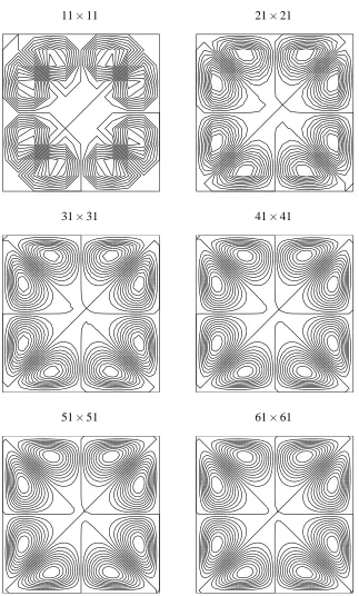
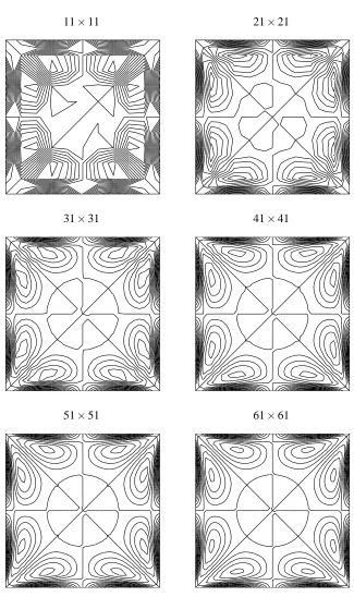
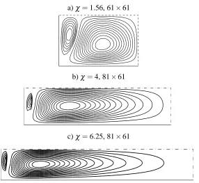
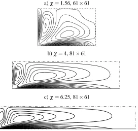
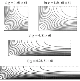
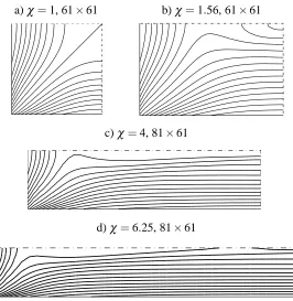
Computations are carried out using γ=0.01 and grids of{11×11,21×21,· · ·,61×61}. Fig. 1 and Fig. 2 show the convergence behaviour of the streamfunction and vorticity fields atχ=1, respectively. It can be seen that the flow is symmetric about the vertical and horizontal centreline and the two fields converge very fast with grid refinement. There are eight vortices in total, where secondary circulations have the same magnitude but different signs (i.e. one vortex is in opposite direction to its two adjacent vortices). Fig. 3 and Fig. 4 show patterns of the secondary flow forχ={1.56,4,6.25}on one quarter of the cross-section. Each quadrant has two vortices, whose patterns and strength strongly depend on the aspect ratio for a given mean primary velocity. Unlike the case of χ =1, where the two vortices are symmetric about the diagonal plane, the case ofχ>1 produces two vortices of different sizes. The vortex near the long wall moves towards the short wall with increasingχ, while the vortex near the short wall is reduced in size. Fig. 5 and Fig. 6 show patterns of the primary flow and the second normal stress difference for all aspect ratios. The 1D-IRBFN Galerkin results are similar to those reported in [Gervang and Larsen (1991); Xue, Phan-Thien, and Tanner (1995)].

4.2 Problem 2: Fully-developed flows of Oldroyd-B fluid in circular tubes

This problem is concerned with the so-called Poiseuille flow in a circular tube. Let R be the radius of the tube. The governing equations Eq. 1 - Eq. 2 and Eq. 19 - Eq. 22 are made dimensionless by scaling lengths by R, velocity components by Q/R2_{, and stress components and pressure by(}µ

n+µp)Q/R3in which Q is the

Oldroyd-B fluid is given by [Pilitsis and Beris (1989)] _∂2_ψ

∂r2 + ∂2_ψ

∂z2 − 1

r

∂ψ ∂r

+ω=0, (63)

α∂_∂2ω

r2 + 1

r

∂ω ∂r −

ω

r2+ ∂2ω

∂z2

=∂

2_T

rz

∂r2 − ∂2_T

rr

∂z∂r −

∂2_T

rz

∂z2 −1

r

_∂

Trr

∂z −

∂T_θθ

∂z

+∂

2_T

zz

∂r∂z−

1

r2Trz+ 1

r

∂Trz

∂r , (64)

where α =µn/(µn+µp)and the inertia terms are set aside. The velocity and stress fields can be obtained

analytically and their exact forms are

e

uz=1−r2,uer=0, (65)

e

Tzz=We(1−α)

_∂ e

uz

∂r

2

,Terz= (1−α)∂_∂u˜_rz,Terr=0, (66)

where We=λQR3is the Weissenberg number. In the present simulation, the length and the radius of the tube are all chosen to be 1. Boundary conditions are prescribed as follows.

• On the centreline:

ψ =ω=Trz=∂

Trr

∂r =

∂Tzz

∂r =

∂Tθθ

∂r =0 (symmetrical conditions)

• On the wall: Through Eq. 11 (uz=1/r(∂ψ/∂r)), the streamfunction value is determined asψ=Q/2π.

Given Q=π/2, one hasψ=1/4. The vorticity value can be obtained using the same procedure as in Problem 1.

• On the inlet and the outlet:

ψi_=ψo_, ∂ψi

∂n =

∂ψo

∂n , ω

i_=ωo_, ∂ωi

∂n =

∂ωo

∂n , T_rri =T_rro, T_rzi =T_rzo, T_zzi =T_zzo, T_θθi =T_θθo ,

where periodicity is taken into account, and superscripts i and o denote the inlet and outlet, respectively.

4.3 Problem 3: Flows of Newtonian and Oldroyd-B fluids in corrugated tubes

The 1D-IRBFN collocation method is further validated through the simulation of flows in corrugated tubes. It is well known that such flows, where their solutions are smooth and there are no inflow/outflow boundary con-ditions applied, are chosen as a benchmark test problem for validating new solvers in computational rheology. Solutions to these flows were reported for several numerical methods, e.g. the pseudospectral finite difference method (PSFD), pseudo-spectral cylindrical finite difference method (PCFD) and full pseudo-spectral method (FCC) by Pilitsis and Beris (1989, 1991, 1992), the spectral method (SM) by Momeni-Masuleh and Phillips (2004), EMME/FEM by Burdette, Coates, Armstrong, and Brown (1989); Rajagopalan, Armstrong, and Brown (1990), EVSS/FEM by Szady, Salamon, Liu, Bornside, and Armstrong (1995), BEM by Zheng, Phan-Thien, Tanner, and Bush (1990), and 2D-IRBFN by Mai-Duy and Tanner (2006).

Fig. 8a shows the flow geometry, where the radius of the corrugated tube along the z axis is given by

rw=R(1−εcos(2πz

L)), (67)

where R is the average radius of an equivalent straight tube, ε the amplitude of the corrugation and L the wavelength. In addition toε, two more characteristic dimensionless numbers are also used. They are the aspect ratio N=R/L and the wave number l; their relation is N=l/(2π). Since the flow is axisymmetric and periodic, only a reduced domain (Fig. 8b) needs be considered for the numerical study.

The streamfunction and vorticity equations as well as the boundary conditions here are similar to those in Problem 2. The governing equations are solved in a stretched cylindrical coordinate system (_br,θ,_bz), where b

r≡r/rwandbz≡z. One important measure for corrugated tube flows is the flow resistance defined as

f Re= 2π∆PR

4

L(µn+µp)Q

, (68)

where∆P is the constant pressure drop per unit cell. 4.3.1 Newtonian fluid

The proposed method is first tested with the case of a Newtonian fluid. With the presence of the inertial term, the vorticity equation Eq. 9 becomes [Pilitsis and Beris (1991)]

_∂2_ω ∂r2 +

1

r

∂ω ∂r −

ω

r2+ ∂2_ω

∂z2

=πRe

2

uz∂ω_∂

z +ur

∂ω ∂r −

ur

r ω

, (69)

where Re is the Reynolds number defined as

Re= 2ρQ

πRµ. (70)

shows streamlines for ε=0.5 and N=0.5, whose structure can be seen to be similar to that in [Pilitsis and Beris (1991)]. As expected, the streamfunction field is symmetric about the widest cross-section of the tube, i.e. z=1/2.

For Re>0, we consider the tube with(ε =0.16,N=0.3)and Re up to a value of 783. Tab. 3 reports f Re for a wide range of Re. Results obtained by the global spectral method [Lahbabi and Chang (1986)], and by the Galerkin finite element method (GFE) and FCC [Pilitsis and Beris (1992)] are also included for comparison purposes. The 1D-IRBFN results approach the FCC ones as the grid is refined. Furthermore, they are in better agreement with the FCC results than the GFE ones. Contour plots for the streamfunction and vorticity are shown in Fig. 10, which look feasible in comparison with those reported in [Lahbabi and Chang (1986); Mai-Duy and Tanner (2006)]. It can be seen that the flows are no longer symmetric. There appears a recirculation. As Re increases, its size grows and its centre moves towards the tube axis.

4.3.2 Oldroyd-B fluid

The Oldroyd-B model is implemented withα=0.85 that is widely used in the literature (e.g. [Pilitsis and Beris (1989)]). Like in [Pilitsis and Beris (1989)], we only consider creeping flows. Taking non-slip and symmetrical boundary conditions into account, the constitutive equations reduce to algebraic equations on the wall and to ODEs on the centreline, respectively. As a result, the stress equations on these boundary lines can be solved separately from the set of stress equations associated with the interior nodes. On the other hand, the value of uz

on the centreline can be obtained by means of L’Hospital’s rule.

In this work, instead of considering ODEs, the values of Trr, Tzz and Tθθ on the centreline are computed by

directly employing 1D-IRBFNs (function interpolation). Those values are regarded as nodal unknowns and they can be found using the symmetric conditions. On each radial grid line zi with i= (2,· · ·,Nz−1), through

Eq. 38, one has

∂Trr(zi,r=0)

∂r =

Nr

∑

j=1

∂ϕj(r=0)

∂r (Trr)i,j =0, (71)

∂Tzz(zi,r=0)

∂r =

Nr

∑

j=1

∂ϕj(r=0)

∂r (Tzz)i,j=0, (72)

∂Tθθ(zi,r=0)

∂r =

Nr

∑

j=1

∂ϕj(r=0)

∂r (Tθθ)i,j=0. (73)

Eq. 71 - Eq. 73 need be solved in conjunction with the set of stress equations associated with the interior nodes. The advantage of this approach is that one can avoid computing velocity derivatives in the constitutive equations on the centreline. We apply a coupled approach to handle the governing equations, in which the resultant nonlinear algebraic set is solved by means of Newton iteration (trust region method).

We=2 is plotted showing the influence of the grid size. As the grid is refined, the smoothness of the computed field is improved and the maximum and minimum values of urremain unchanged. A grid density of 21×21

appears to be sufficient for computing urat We=2. Fig. 12 shows the behaviour of Trzwith increasing We. At

high values of We, steep layers are formed in the area close to the wall. This behaviour can also be seen for Tzz

as shown in Fig. 13. In Fig. 14a, the 1D-IRBFN solution is shown to converge up to We=6 and the values of

f Re are in good agreement with the benchmark solution [Pilitsis and Beris (1992)] (solutions in [Pilitsis and

Beris (1992)] reported only for three values of We, namely 0, 1.2071 and 3.6213). Denser grids are required for higher-We solutions. It is noted that the two coarse grids, 11×11 and 21×21, fail to yield a convergent solution for high values of We.

In the case of moderate corrugation amplitude and moderate wave length (ε =0.1, N=0.16), three grids of 11×11, 21×21 and 31×31 are employed. The plot of f Re versus We is shown in Fig. 14b. It can be seen that a convergent f Re solution is obtained up to We=7 using 11×11, We=8 using 21×21, and We=18 using 31×31. Other remarks here are similar to those in the previous case (ε=0.1, N=0.5).

5 Concluding remarks

In this paper, viscoelastic flows in rectangular ducts and in straight and corrugated tubes are simulated with 1D-IRBFN-based Galerkin/Collocation techniques. Instead of using low-order polynomials, the trial functions in the Galerkin and point-collocation formulations are presently implemented with 1D-IRBFs. Boundary treat-ments especially for those on the centreline using 1D-IRBFNs are discussed in detail. The 1D-IRBFN results, which are obtained for a wide range of the Weissenberg number, are in good agreement with the exact/numerical solutions available in the literature. Implementation of the constitutive equations in their matrix logarithm form for higher We solutions in the context of 1D-IRBFNs is currently under investigation and will be reported in future work.

Acknowledgement: D. Ho-Minh would like to thank the CESRC, FoES and USQ for a postgraduate schol-arship. This research is supported by the Australian Research Council.

References

Atluri, S. N.; Han, Z. D.; Rajendran, A. M. (2004): A New Implementation of the Meshless Finite Volume Method, Through the MLPG “Mixed” Approach. CMES: Computer Modeling in Engineering & Sciences, vol. 6 (6), pp. 491–514.

Atluri, S. N.; Han, Z. D.; Shen, S. (2003): Meshless Local Petrov-Galerkin (MLPG) Approaches for Solving the Weakly-Singular Traction & Displacement Boundary Integral Equations. CMES: Computer Modeling in

Engineering & Sciences, vol. 4 (5), pp. 507–518.

Burdette, S. R.; Coates, P. J.; Armstrong, R. C.; Brown, R. A. (1989): Calculations of viscoelastic flow through an axisymmetric corrugated tube using the explicitly elliptic momentum equation formulation (EEME).

Journal of Non-Newtonian Fluid Mechanics, vol. 33, pp. 1–23.

Criminale, W. O. J.; Ericksen, J. L.; Filbey, G. L. J. (1957): Steady shear flow of non-Newtonian Fluids.

Archive for Rational Mechanics and Analysis, vol. 1(1), pp. 410–417.

Crochet, M. J. (1989): Numerical simulation of viscoelastic flow: A review. Rubber Chemistry and Technology, vol. 62, pp. 426–455.

Crochet, M. J.; Davies, A. R.; Walters, K. (1984): Numerical simulation of non-Newtonian flow. Elsevier

Science Publishers.

Crochet, M. J.; Walters, K. (1983): Numerical methods in non-Newtonian fluid mechanics. Annual Review

of Fluid Mechanics, vol. 15, pp. 241–260.

Gervang, B.; Larsen, P. (1991): Secondary flows in straight ducts of rectangular cross section. Journal of

Non-Newtonian Fluid Mechanics, vol. 39, pp. 217–237.

Green, G. E.; Rivlin, R. S. (1956): Steady flow of non-Newtonian fluids through tubes. Quaterfly of Applied

Mathematics, vol. 14, pp. 299–308.

Ho-Minh, D.; Mai-Duy, N.; Tran-Cong, T. (2009): A Galerkin-RBF approach for the streamfunction-vorticity-temperature formulation of natural convection in 2D enclosured domains. CMES: Computer

Model-ing in EngineerModel-ing & Sciences, vol. 44, pp. 219–248.

Kansa, E. J. (1990): Multiquadrics - A scattered data approximation scheme with applications to computa-tional fluid dynamics I. Surface approximations and partial derivative estimates. Computers and Mathematics

with Applications, vol. 19, pp. 127–145.

Lahbabi, A.; Chang, H. C. (1986): Flow in periodically constricted tubes: Transition to inertial and nonsteady flows. Chemical Engineering Science, vol. 41 (10), pp. 2487–2505.

Mai-Duy, N.; Ho-Minh, D.; Tran-Cong, T. (2009): A Galerkin approach incorporating integrated radial basis function networks for the solution of biharmonic equations in two dimensions. International Journal of

Computer Mathematics, vol. 86 (10-11), pp. 1746–1759.

Mai-Duy, N.; Tanner, R. I. (2006): Computing non-Newtonian fluid flow with radial basis function networks.

International Journal for Numerical Methods in Fluids, vol. 48, pp. 1309 –1336.

Mai-Duy, N.; Tran-Cong, T. (2001): Numerical solution of differential equations using multiquadric radial basis function networks. Neural Networks, vol. 14, pp. 185–199.

Mai-Duy, N.; Tran-Cong, T. (2007): A Cartesian-grid collocation method based on radial basis function networks for solving PDEs in irregular domains. Numerical Methods for Partial Differential Equations, vol. 23, pp. 1192–1210.

Mai-Duy, N.; Tran-Cong, T. (2009): A Cartesian-Grid Discretisation Scheme Based on Local Integrated RBFNs for Two-Dimensional Elliptic Problems. CMES: Computer Modeling in Engineering & Sciences, vol. 51 (3), pp. 213–238.

Momeni-Masuleh, S. H.; Phillips, T. N. (2004): Viscoelastic flow in an undulating tube using spectral methods. Computers & Fluids, vol. 33, pp. 1075–1095.

Owens, R. G.; Phillips, T. N. (2002): Computational Rheology. Imperial College Press.

Phillips, T. N.; Owens, R. G. (1997): A mass conserving multi-domain spectral collocation method for the Stokes problem . Computers & Fluids, vol. 8, pp. 825–840.

Pilitsis, S.; Beris, A. N. (1989): Calculation of Steady-state viscoelastic flow in an undulating tube. Journal

of Non-Newtonian Fluid Mechanics, vol. 31, pp. 231–287.

Pilitsis, S.; Beris, A. N. (1991): Viscoelastic flow in an undulating tube. Part II. Effects of high elasticity, large amplitude of undulation and inertia. Journal of Non-Newtonian Fluid Mechanics, vol. 39, pp. 375–405.

Pilitsis, S.; Beris, A. N. (1992): Pseudospectral calculations of viscoelastic flow in a periodically constricted tube . Computer Methods in Applied Mechanics and Engineering, vol. 98 (3), pp. 307–328.

Rajagopalan, D.; Armstrong, R. C.; Brown, R. A. (1990): Finite element methods for calculation of steady, viscoelastic flow using constitutive equations with a Newtonian viscosity. Journal of Non-Newtonian Fluid Mechanics, vol. 36, pp. 159–192.

Schaback, R. (1995): Error estimates and condition numbers for radial basis function interpolation. Advances

in Computational Mathematics, vol. 3, pp. 251–264.

Sellountos, E. J.; Sequeira, A.; Polyzos, D. (2010): Solving Elastic Problems with Local Boundary Integral Equations (LBIE) and Radial Basis Functions (RBF) Cells. CMES: Computer Modeling in Engineering & Sciences, vol. 57 (2), pp. 109–136.

S ˇarler, B. (2005): A Radial Basis Function Collocation Approach in Computational Fluid Dynamics. CMES:

Computer Modeling in Engineering & Sciences, vol. 7 (2), pp. 185–193.

Szady, M. J.; Salamon, T. R.; Liu, A. W.; Bornside, D. E.; Armstrong, R. C. (1995): A new mixed finite element method for viscoelastic flows governed by differential constitutive equations. Journal of

Non-Newtonian Fluid Mechanic, vol. 59, pp. 215–243.

Tanner, R. I.; Xue, S.-C. (2002): Computing transient flows with high elasticity. Korea-Australia Rheology

Tran-Canh, D.; Tran-Cong, T. (2002): Computation of viscoelastic flow using neural networks and stochastic simulation. Korea-Australia Rheology Journal, vol. 14 (4), pp. 161–174.

Tran-Cong, T.; Mai-Duy, N.; Phan-Thien, N. (2002): BEM-RBF approach for viscoelastic flow analysis.

Engineering Analysis with Boundary Elements, vol. 26 (9), pp. 757–762.

Xue, S. C.; Phan-Thien, N.; Tanner, R. I. (1995): Numerical study of secondary flows of viscoelastic fluid in strait pipes by an implicit finite volume method. Journal of Non-Newtonian Fluid Mechanic, vol. 59, pp. 191–213.

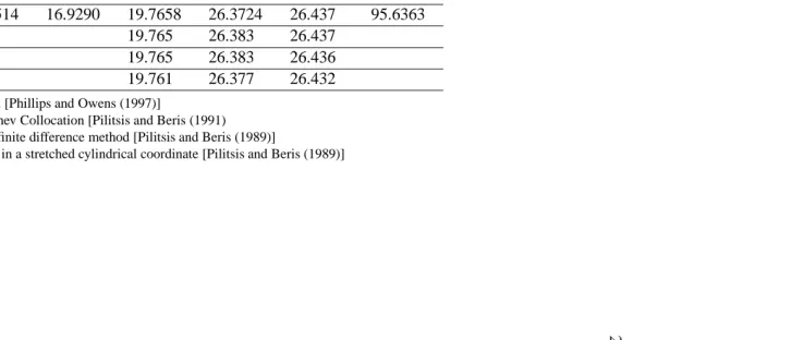
Table 1: Problem 2: Grid-convergence study at We=9.

Relative L2errors

Grid uz Tzz Trz

2

3

and N

ε 0.1 0.1 0.2 0.286 0.3 0.5

N 0.5 0.1592 0.1042 0.2333 0.1592 0.5 Present method

21×21 17.71385 16.91518 19.75360 26.33921 26.40423 95.18132 41×41 17.73548 16.92656 19.76213 26.37003 26.42937 95.51616 61×61 17.74106 16.92760 19.76351 26.37759 26.43378 95.61778

SMa 17.7514 16.9290 19.7658 26.3724 26.437 95.6363

FCCb 19.765 26.383 26.437

PSFDc 19.765 26.383 26.436

PCFDd 19.761 26.377 26.432

a _{Spectral method [Phillips and Owens (1997)]}

b _{Fourier-Chebyshev Collocation [Pilitsis and Beris (1991)} c _{Pseudospectral/finite difference method [Pilitsis and Beris (1989)]}

2

4

Re

0 12 22.6 51 73 132 207.4 264 387.2 783

Present method

21×21 26.49503 27.22021 28.59313 31.80464 33.48944 36.61126 39.04828 40.34471 42.48868 46.02994 31×31 26.47991 27.20798 28.57514 31.78472 33.46705 36.56876 39.00632 40.29224 42.40401 45.66516 41×41 26.46953 27.19921 28.56523 31.77200 33.45333 36.53881 38.99009 40.27630 42.38337 45.62292 51×51 26.46298 27.19314 28.55838 31.76329 33.44396 36.51618 38.97686 40.26089 42.37057 45.60680

2D IRBFNa 26.4445 27.1773 28.5535 31.7511 33.4538 36.5424 38.996 40.3044 42.4595 45.7402 GFEb 26.4193 27.0911 28.4433 31.6984 33.4039 36.5392 38.933 40.1544 42.1112 45.0734 FCCc 26.4484 27.1791 28.5536 31.7484 33.4488 36.5264 38.9607 40.2446 42.3479 45.5828 a _{2D-Integated Radial basis function network [Mai-Duy and Tanner (2006)]}

11×11 21×21

31×31 41×41

51×51 61×61

11×11 21×21

31×31 41×41

51×51 61×61

a)χ=1.56, 61×61

b)χ=4, 81×61

c)χ=6.25, 81×61

a)χ=1.56, 61×61

b)χ=4, 81×61

c)χ=6.25, 81×61

a)χ=1, 61×61 b)χ=1.56, 61×61

c)χ=4, 81×61

d)χ=6.25, 81×61

a)χ=1, 61×61 b)χ=1.56, 61×61

c)χ=4, 81×61

d)χ=6.25, 81×61

a) Velocity b) Shear stress

0 0.2 0.4 0.6 0.8 1

0 0.1 0.2 0.3 0.4 0.5 0.6 0.7 0.8 0.9 1 analytical computed r-Coordinate uz

0 0.2 0.4 0.6 0.8 1

−1.8 −1.6 −1.4 −1.2 −1 −0.8 −0.6 −0.4 −0.2 0 analytical computed r-Coordinate Trz

c) Normal stress difference d) Normal stress difference

0 0.2 0.4 0.6 0.8 1

−5 0 5 10 15 20 25 analytical computed r-Coordinate N1 = Tzz − Trr We=0.5 We=1 We= 2 We= 3

0 0.2 0.4 0.6 0.8 1

−10 0 10 20 30 40 50 60 70 80 analytical computed r-Coordinate N1 = Tzz − Trr We=4 We= 6 We= 8 We= 10

Figure 7: Problem 2: Profiles of velocity and stress on the middle plane z=0.5 computed at several values of

We using a grid of 21×21. It is noted that uzand Trzare independent of We and their corresponding computed

a) Geometry

b) Reduced domain and discretisation

ψ

Re=0

ψ ω

Re=132

ψ ω

Re=397.2

ψ ω

Re=783

ψ ω

11×11 21×21

0.048 −0.049

0.048 −0.049

31×31 41×41

0.048 −0.049

0.048 −0.049

Figure 11: Problem 3, Oldroyd-B fluid,ε=0.1, N=0.5: Contour plots for urat We=2 using several grids.

We=0 We=1

0.000 −0.323

0.000 −0.463

We=3 We=6

0.370 −0.855

0.976 −1.422

Figure 12: Problem 3, Oldroyd-B fluid,ε =0.1, N=0.5: Contour plots for Trz at four values of We using a

31×31 41×41

7.274 −0.015

8.076 −0.006

Figure 13: Problem 3, Oldroyd-B fluid,ε=0.1, N=0.5: Contour plots for Tzzat We=6 using grids of 31×31

a)ε=0.1, N=0.5

0 5 10 15

17.5 17.6 17.7 17.8 17.9 18 18.1 18.2 18.3 18.4 18.5

Present study (31 × 31) Present study (41 × 41) FCC (16 × 33)

We

fR

e

b)ε=0.1, N=0.16

0 5 10 15 20 25 30

16.5 17 17.5 18 18.5

Present study (11 × 11) Present study (21 × 21) Present study (31 × 31)

We

fR

e