C
2011. The American Astronomical Society. All rights reserved. Printed in the U.S.A.
MODELING
KEPLER
TRANSIT LIGHT CURVES AS FALSE POSITIVES: REJECTION OF BLEND SCENARIOS
FOR KEPLER-9, AND VALIDATION OF KEPLER-9 d, A SUPER-EARTH-SIZE PLANET IN
A MULTIPLE SYSTEM
Guillermo Torres1, Fran ¸cois Fressin1, Natalie M. Batalha2, William J. Borucki3, Timothy M. Brown4,
Stephen T. Bryson3, Lars A. Buchhave5, David Charbonneau1, David R. Ciardi6, Edward W. Dunham7,
Daniel C. Fabrycky1, Eric B. Ford8, Thomas N. Gautier III9, Ronald L. Gilliland10, Matthew J. Holman1, Steve B. Howell11, Howard Isaacson12, Jon M. Jenkins13, David G. Koch3, David W. Latham1, Jack J. Lissauer3,
Geoffrey W. Marcy14, David G. Monet15, Andrej Prsa16, Samuel N. Quinn1, Darin Ragozzine1, Jason F. Rowe3,19,
Dimitar D. Sasselov1, Jason H. Steffen17, and William F. Welsh18
1Harvard-Smithsonian Center for Astrophysics, Cambridge, MA 02138, USA;[email protected] 2San Jose State University, San Jose, CA 95192, USA
3NASA Ames Research Center, Moffett Field, CA 94035, USA 4Las Cumbres Observatory Global Telescope, Goleta, CA 93117, USA 5Niels Bohr Institute, Copenhagen University, DK-2100 Copenhagen, Denmark
6NASA Exoplanet Science Institute/Caltech, Pasadena, CA 91125, USA 7Lowell Observatory, Flagstaff, AZ 86001, USA
8University of Florida, Gainesville, FL 32611, USA
9Jet Propulsion Laboratory/California Institute of Technology, Pasadena, CA 91109, USA 10Space Telescope Science Institute, Baltimore, MD 21218, USA
11National Optical Astronomy Observatory, Tucson, AZ 85719, USA 12San Francisco State University, San Francisco, CA 94132, USA 13SETI Institute/NASA Ames Research Center, Moffett Field, CA 94035, USA
14University of California, Berkeley, CA 94720, USA 15US Naval Observatory, Flagstaff Station, Flagstaff, AZ 86001, USA
16Villanova University, Villanova, PA 19085, USA
17Fermilab Center for Particle Astrophysics, P.O. Box 500, Batavia, IL 60510, USA 18San Diego State University, San Diego, CA 92182, USA
Received 2010 September 1; accepted 2010 November 12; published 2010 December 28
ABSTRACT
Light curves from the KeplerMission contain valuable information on the nature of the phenomena producing the transit-like signals. To assist in exploring the possibility that they are due to an astrophysical false positive, we describe a procedure (BLENDER) to model the photometry in terms of a “blend” rather than a planet orbiting a star. A blend may consist of a background or foreground eclipsing binary (or star–planet pair) whose eclipses are attenuated by the light of the candidate and possibly other stars within the photometric aperture. We apply
BLENDERto the case of Kepler-9 (KIC 3323887), a target harboring two previously confirmed Saturn-size planets (Kepler-9 b and Kepler-9 c) showing transit timing variations, and an additional shallower signal with a 1.59 day period suggesting the presence of a super-Earth-size planet. UsingBLENDERtogether with constraints from other follow-up observations we are able to rule out all blends for the two deeper signals and provide independent validation of their planetary nature. For the shallower signal, we rule out a large fraction of the false positives that might mimic the transits. The false alarm rate for remaining blends depends in part (and inversely) on the unknown frequency of small-size planets. Based on several realistic estimates of this frequency, we conclude with very high confidence that this small signal is due to a super-Earth-size planet (Kepler-9 d) in a multiple system, rather than a false positive. The radius is determined to be 1.64+0.19
−0.14R⊕, and current spectroscopic observations are as yet insufficient to establish its mass.
Key words: binaries: eclipsing – planetary systems – stars: individual (Kepler-9, KIC 3323887, KOI-377) – stars: statistics
Online-only material:color figures
1. INTRODUCTION
The Kepler Mission, launched in March of 2009, was de-signed to address the important question of the frequency of Earth-size planets around Sun-like stars, and to characterize ex-trasolar transiting planets through a 3.5 year program of very precise photometric monitoring of∼156,000 stars (Koch et al.
2010). Science results from the mission have already begun to appear (Borucki et al.2010,2011; Steffen et al. 2010). As shown already by ground-based surveys for transiting planets,
19NASA Postdoctoral Program Fellow.
considerable effort is required to validate candidates detected photometrically. This is because false positives usually outnum-ber true planetary systems by a large factor, which is about 10:1 for the most successful surveys from the ground, but is not yet well characterized forKepler. The follow-up efforts by the Keplerteam have been summarized by Batalha et al. (2010).
binary (“blends”). However, for faint candidates (V > 14) high-resolution, high signal-to-noise ratio (S/N) spectroscopy becomes prohibitively expensive in terms of telescope time. Even for brighter candidates, the reflex motion of the star due to an Earth-mass planet can sometimes be below the radial-velocity detection limit, making spectroscopic confirmation very difficult or impossible. The question then becomes how to validate these candidates, particularly the ones with small planets that are precisely among the most interesting.
A number of other tests have been developed that can aid in understanding the nature of the candidate, and that rely on the long-term and nearly continuous photometric monitoring of Kepler, as well as the very high astrometric precision achieved in determining the centroids of the stars (see also Steffen et al.
2010). These tests include: (1) verifying that alternating events have the same depth, which they may not if the signal is due to a background eclipsing binary; (2) checking for the presence of shallow secondary eclipses, which are common in eclipsing bi-naries but are not expected for the smallest planets; (3) checking for ellipsoidal variations, which could be another sign of a blend; (4) checking for changes in the centroid positions correlated with the brightness changes, which, if detected, might indicate a blend, or at the very least, a crowded aperture. This is a power-ful diagnostic that is able to disprove many background blends. In addition to these tests, high-resolution imaging is an important tool to identify neighboring stars that might be eclipsing binaries with the potential to cause the transit-like signals. The photometric aperture of Kepler is large enough (typically many arcseconds across) that it usually includes other stars in addition to the candidate, which increases the risk of such blends. In some cases, near-infrared observations with WarmSpitzercan allow one to reject the planet hypothesis if the transit depth at 3.6μm or 4.5μm is significantly different from that in theKeplerband. Such a signature might result from a blend with an eclipsing binary of a different spectral type than the candidate.20
Even with this extensive battery of tests it may still be difficult or impossible to provide validation for many of the most interesting planet candidates discovered by Kepler. For example, blend scenarios involving an eclipsing binary or an eclipsing star–planet pair physically associated with the candidate (hierarchical triple systems) and in a long-period orbit around their common center of mass would often be spatially unresolved from the ground. These configurations may also not be detectable spectroscopically, and would likewise not produce any measurable centroid motion. Therefore, it is imperative to take advantage of all the information available in vetting candidates.
With this as our motivation, we describe here the use of theKepler light curves themselves in a different way to help discriminate between true planetary transits and a large variety of possible blend scenarios, on a much more quantitative basis than simple back-of-the-envelope calculations could provide. The technique tests these scenarios by directly modeling the light curves as blends and has considerable predictive power that allows the expected properties of the various configurations to be tested against other information that may be available. Both hierarchical triples and background blends can be explored. A restricted application of this type of modeling to Kepler
20For Earth-size planets, the amplitude of the signal in theKeplerband is very
small and possibly below the detection threshold forSpitzer. However, a blend with a late-type binary could produce a much deeper eclipse at longer wavelengths that may be detectable in the near-infraredSpitzerbands.
has already been made for the five multi-planet candidates announced recently by Steffen et al. (2010). For the present paper we have chosen to illustrate the full potential of the method, which we refer to as BLENDER, by applying it to the unique case of Kepler Object of Interest 377 (KOI-377, henceforth Kepler-9). This is a multi-planet system reported and described in detail by Holman et al. (2010), withthree low-amplitude periodic signals in its light curve. We have selected this system for two main reasons. On the one hand, it represents the first unambiguous detection of transit timing variations (TTVs) in an extrasolar planet, with a pattern of variation seen in two of its signals (Kepler-9 b and Kepler-9 c) that constitutes irrefutable evidence that the objects producing them are bona fide planets. This offers an ideal opportunity to test BLENDER
because their true nature is already known. On the other hand, the third signal (KOI-377.03)21 is small enough that it would
correspond to a super-Earth, but validation of its planetary origin is not yet in hand. Should it be validated, Kepler-9 would become an even more remarkable laboratory for the study of the architecture of planetary systems involving small planets. Thus, exploring the wide range of possible blend configurations that might mimic this shallow signal is of the greatest interest for determining its true nature.
Kepleris likely to find many other candidate transiting planets similar to KOI-377.03, for which final validation by other means is not currently feasible, either because the expected radial-velocity signal is too small or because Doppler measurements are otherwise complicated due to the star being chromospheri-cally active, rapidly rotating, or too faint. With the application to Kepler-9 we show that our light-curve modeling technique is a powerful tool for exploring astrophysical false positive scenar-ios that is complementary to other diagnostics, and should play an important role in the discovery of Earth-size planets around otherKeplertargets.
2. SIMULATING FALSE POSITIVES WITHBLENDER
In general the detailed shape of a light curve displaying transit-like events can be expected to contain useful constraints on possible blend scenarios that might be responsible for those signals. With photometry of the quality of that provided by Kepler, those constraints can be quite strong and may be used to exclude many blend configurations and provide support for the planetary hypothesis. It is thus highly desirable to take advantage of this information, particularly since it relies only on observations already in hand.
The idea behindBLENDERis to compare the transit photometry of a candidate against synthetic light curves produced by an eclipsing binary that is included within the photometric aperture ofKepler, and is contaminating the light of the candidate. The usually deep eclipses of the binary are attenuated by the light of the candidate, and reduced in depth so that they appear transit-like. In principle there is an enormous range of possible binary configurations that could mimic all of the features of true planetary transits, including not only their depth, but also the total duration and the length of the ingress and egress phases. Generally, it is only with detailed modeling that these can be ruled out. Possible scenarios include not only background eclipsing binaries, but also hierarchical triples, i.e., an eclipsing
21 The name of this candidate follows the convention of theKeplerMission in
binary physically associated with the candidate in a wide orbit around their common center of mass.
The basic procedure for simulating light curves withBLENDER
was described in detail by Torres et al. (2004), and further changes and enhancements are discussed below. Briefly, the brightness variations of an eclipsing binary are generated with the binary light-curve code EBOP (Popper & Etzel 1981), based on the Nelson–Davis–Etzel model (Nelson & Davis1972; Etzel 1981), and then diluted by the light of the candidate for comparison with the Keplerobservations. Effects such as limb darkening, gravity brightening, mutual reflection, and oblateness of the binary components are included. The objects composing the binary are referred to as the “secondary” and “tertiary,” and the candidate is the “primary.” The properties of each object needed to generate the light curves (brightness and size) are taken from model isochrones by Marigo et al. (2008), parameterized in terms of their stellar mass.22 For the
primary star the appropriate isochrone is selected by using as constraints the effective temperature, surface gravity, and metallicity determined spectroscopically. We assign also a mass and a radius from this isochrone, although these characteristics are irrelevant for generating the model light curves. We then read off the intrinsic brightness of the star (absolute magnitude) in theKeplerpassband, which is the only property needed by
BLENDER. The brightness of the primary is held fixed throughout all simulations. The parameters of the binary components are allowed to vary freely over wide ranges in order to provide the best match to the Kepler photometry in a χ2 sense, subject only to the condition that the two stars lie on the same isochrone, as expected from coeval formation. To read off their properties (absolute magnitude and size) we use the mass as an intermediate variable. The specific isochrone adopted for the binary depends on the configuration: for hierarchical triple scenarios we adopt the same age and chemical composition as the primary, whereas for background binaries the isochrone can be different. TheKeplerlight curve itself does not provide a useful constraint on the age or metallicity of the binary in the background case, so a typical choice is a model for solar metallicity and a representative age for the field such as 3 Gyr. For background binary scenarios the distance between the binary and the main star is parameterized for convenience in terms of the difference in distance modulus,Δδ. The inferred distance between the primary star and the observer will vary from blend to blend because we constrain the combined brightness of all components of the blend to match the measured apparent brightness of the target.BLENDER is also able to account for differential extinction between the primary and the binary, which can have a non-negligible effect in some cases given the relatively low Galactic latitude of theKeplerfield.
Early versions of BLENDER have been used occasionally in recent years to examine transiting planet candidates from ground-based surveys such as OGLE, TrES, and HATNet (see, e.g., Torres et al. 2004, 2005; Mandushev et al. 2005; O’Donovan et al. 2006; Bakos et al. 2007), as well as from CoRoT (F. Fressin et al. 2011, in preparation). These studies have exploited the predictive power of BLENDER to estimate further properties of the blend scenarios, by testing them against
22 This particular set of isochrones was chosen because it reaches lower
masses than other models (nominally 0.15M, which we have extrapolated slightly for this application to 0.10M, near the brown dwarf limit), and because a convenient web tool provided by the authors allows easy
interpolation in both age and metallicity (http://stev.oapd.inaf.it/cgi-bin/cmd). Additionally, isochrone magnitudes are available in a variety of passbands including theKeplerandSpitzerpassbands, as well as Sloan and 2MASS.
complementary information such as color indices, optical/near-infrared spectroscopy, or near-optical/near-infrared photometry fromSpitzer. For the application toKepler, several important modifications have been made to BLENDER, including the following: (1) the ability to generate light curves integrated over the 29.4 minute effective duration of an observation when using long-cadence data. This changes the shape of the transits significantly, given the high precision of the Kepler photometry and the relatively short timescales of the events (see Gilliland et al.
2010; Kipping 2010); (2) de-trending of the original Kepler light curves with a 1 day running median to remove instrumental effects, and rejection of outliers; (3) the use of model isochrones specific to the Kepler passband, kindly computed for us by L. Girardi.BLENDERcan now also use proper limb-darkening coefficients for the same band, as opposed to an approximation to the Keplerpassband such as the JohnsonRfilter, which is considerably narrower.Keplerlimb-darkening coefficients have been computed by Sing (2010) and also A. Prsa;23 (4) extension
to any optical or near-infrared passband. In particular, for any scenario explored withBLENDER, light curves can be computed at other wavelengths such as the 3.6μm and 4.5μm passbands of the IRAC instrument on WarmSpitzer, in order to further test the blend hypothesis. Additionally,BLENDERcan predict the overall color of a blend in any pair of passbands, including the effects of differential reddening for background or foreground scenarios. These colors may then be compared with the measured colors of a target. Extinction at different wavelengths is computed following the prescription by Cardelli et al. (1989); (5) the ability to have the tertiary be a (dark) planet instead of a star, in which case the corresponding free parameter becomes the radius of the planet rather than the tertiary mass. The mass of the planet has little effect on the light curves in most cases, but can nevertheless be set to any value;24(6) the ability to include extra
light from other stars that may be present in theKepleraperture, which further dilutes the intrinsic signatures from the eclipsing binary; (7) the ability to model systems with eccentric orbits. Eccentricity changes the orbital velocities during transit, and can therefore affect the size (mass) of stars that allow satisfactory fits to the light curve.
When exploring blend scenarios involving hierarchical triple systems, the free parameters of the problem are the mass of the secondary, the mass of the tertiary (or its radius, if a planet), and the inclination angle. A fourth variable, the difference in distance modulus, is added for background blends. These quantities are typically stepped over wide ranges in a grid pattern to fully map the χ2 surface. For the application to Kepler-9 below, stellar masses are allowed to vary along the isochrones between 0.1M
and 1.4M, although at the larger values the observed duration of the transits is already difficult to match unless the events are highly grazing, in which case the shape would be very different. For planetary tertiaries the radii are allowed to be as large as 1.8RJup; values higher than this have not been observed.
3. APPLICATION TO KEPLER-9
Kepler-9 (KIC 3323887, 2MASS 19021775+3824032) is a relatively faint star compared to typical ground-based
23 http://astro4.ast.villanova.edu/aprsa/?q=node/8
24 We note that this option ofBLENDERimplicitly allows to consider white
transit hosts (Kepler magnitude Kp = 13.8), which was ob-served by the mission beginning in the first quarter of oper-ations, and presents three distinct periodic signals in its light curve. The two with the largest amplitudes have periods of 19.24 days (Kepler-9 b) and 38.91 days (Kepler-9 c), and bright-ness decrements of 6.5 and 6.0 mmag, respectively. The third signal (KOI-377.03) is much shallower (0.2 mmag) and repeats every 1.59 days. The two longer periods are within 2.5% of being in a 2:1 ratio, and both objects display obvious TTVs that are anti-correlated, clearly indicating they are interacting gravi-tationally and therefore orbit the same star, and are planetary in nature (see Holman et al.2010). The estimated radii are quite similar to that of Saturn, and the masses are somewhat smaller than Saturn, based on available radial-velocity measurements constrained by transit times and durations. The short-period signal has one of the smallest amplitudes detected byKepler, and may well correspond to a third, super-Earth-size planet in the system, with an estimated radius of only∼1.5R⊕(Holman et al.2010). However, because it shows no TTVs related to the other two planets (nor is expected to, on dynamical grounds), and is predicted to induce only a very small reflex velocity on the parent star that may be below detection for such a faint object, the true origin of this signal has not yet been established.
In the absence of the crucial evidence of TTVs, each of the two largest signals—and indeed the third signal as well—could in principle be due to a different blend.25 Therefore, as an
illustration of the application ofBLENDER, we model the light curve of Kepler-9 at each period separately, as we would any candidate with a single period, and we account for possible blends at the other periods by incorporating extra dilution consistent with those other scenarios. The goal for the two largest signals is to demonstrate, as a sanity check, thatBLENDER
would be able to rule out blends in similar cases where confirmation is lacking, which Kepler is expected to find in significant numbers. For the third signal of unknown nature, the application ofBLENDERshould provide valuable evidence one way or the other.
3.1. Stellar Properties and Photometry
Kepler-9 is a solar type star. The spectroscopic properties of the primary are adopted from Holman et al. (2010):Teff = 5777±61 K, logg=4.49±0.09, and [Fe/H]=+0.12±0.04. With these parameters, a comparison with the stellar evolution models of Marigo et al. (2008) yields a stellar mass ofM = 1.07±0.05M, a radius ofR=1.02±0.05R, and an age of about 1 Gyr, along with the absolute magnitude in theKepler band. Only the latter is used byBLENDERand is held fixed in our modeling. The distance to the star estimated from the same models is about 650 pc, ignoring extinction. Uncertainties in the brightness of the primary stemming from errors inTeff, logg, and [Fe/H] are small. For example, the error in logg, which has the most direct influence on the intrinsic brightness, translates to an uncertainty of little more than 0.1 mag in the absolute magnitude. This has an insignificant impact on our results.
25Unlikely as it may seem to have three different blends operating in the same
system, the large photometric aperture, nearly uninterrupted monitoring, very high photometric precision, and long-term coverage ofKeplercoupled with the large number of targets observed makes it more sensitive to picking up odd cases such as this, so they should not be completely ruled out. An example already exists among the five multi-planet candidates recently reported by Steffen et al. (2010), in which one of the systems (KOI-191) presents three transit-like signals, and one of those signals (0.4 mmag depth) has been shown to be due to a background eclipsing binary 2.6 mag fainter than the target, located 1.5 arcsec away.
The photometry used here consists of the long-cadence measurements gathered for Kepler-9 during Kepler quarters 1, 2, and 3, spanning 218 days, and was treated slightly differently than indicated earlier for a genericKeplercandidate because of the complications stemming from the TTVs. Using the binary FITS tables from MAST (Multimission Archive at STScI, http://archive.stsci.edu/kepler/), the “raw” aperture photometry for each quarter was first de-trended using a moving cubic polynomial fit robustly to out-of-transit data, with a sliding window of 999 minutes before and after each individual datapoint. This technique removes long-term trends due to stellar activity or instrumental errors, but retains the properties of each transit light curve. Statistically significant outliers were removed.
For the two long-period signals, simple folding will not create an accurate light curve because of the strong TTVs. Instead, we used a “shift-and-stack” technique, in which each transit event is displaced so that it is centered at “time” zero using the measured transit times from Holman et al. (2010). Along with the measurements in transit, nearly a full cycle of out-of-transit data was also shifted. Specifically, we shifted nearly 25% of an orbital cycle before the transit, and nearly 75% after the transit. This preserves any curvature outside of eclipse, and in principle would also retain any secondary eclipses, both of which can provide useful constraints when modeling the light curve withBLENDER. We note, however, that the strong TTVs would be accompanied by shifted secondary eclipses in a way that can only be predicted by full numerical integration. This shift-and-stack technique would not align secondary eclipses correctly and thus their depth would need to be significant in each individual event to be noticed. There is no sign of secondary eclipses at these periods in the data at the 10−4level, as expected from the planetary nature of the objects, and thus the failure of the shift-and-stack technique to correctly add up the secondary eclipses does not affect our results. After shifting, all the transit and out-of-transit data were “stacked” together and each data point was given a time relative to time zero at the center of each transit event. This was done separately for the 19 day and 39 day signals. We have been careful not to use a full cycle of out-of-transit data to avoid using any photometric measurements more than once in the input light curve.
For the 1.6 day signal that repeats at regular intervals (since it shows no TTVs), we created a light curve by simply masking out the transits at the other two periods.
3.2. Additional Observations for False Positive Rejection
Figure 1.Image of Kepler-9 from the HIRES guider camera on the Keck I telescope, obtained in seeing of 0.9 and clear skies. Companions within 15are labeled as in Table1. The scale of the image is 0.30 pixel−1. Also indicated are
the optimal photometric aperture (darker gray area of 8 pixels, used to extract the Keplerphotometry) and the target aperture mask (lighter gray area of 31 pixels, used to measure centroids) forKeplerquarter 3.
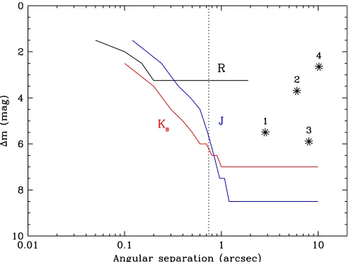
Speckle observations of Kepler-9 were carried out on 2010 June 18 with the WIYN 3.5 m telescope located on Kitt Peak. They were taken with a two-color EMCCD speckle camera using narrow-band filters 40 nm wide centered at 562 nm and 692 nm. We refer loosely to these passbands asVandR. The native seeing was 0.7. No companions withΔm3.25 mag (R band) are present in the field of view centered on the target out to 1.8, at the 5σconfidence level. Inside of 0.2 the sensitivity is reduced, but still allows to rule out brighter companions down to the diffraction limit of 0.04–0.05 (see Figure2). Details of the follow-up speckle observations in the context of theKepler Mission are described in more detail by S. Howell et al. (2011, in preparation).
Additionally, Kepler-9 was observed on 2010 July 2 at the Palomar Hale 200 inch telescope with the near-infrared adaptive optics (AO) PHARO instrument (Hayward et al.2001), a 1024×1024 Rockwell HAWAII HgCdTe array detector. Observations were made in theJ(1.25μm) andKs(2.145μm) bands. The field of view was approximately 20×20, and the scale was 25.1 mas per pixel. The AO system guided on the primary target itself, and produced Strehl ratios of 0.05 at J and 0.3 at Ks. The central cores of the resulting point-spread functions had widths of FWHM = 0.12 at J and FWHM=0.10 atKs. The closer of the companions seen earlier in the Keck images were easily detected, and we list them all
Figure 2.Sensitivity to faint companions near Kepler-9 from our imaging observations. Any companions above the curves are bright enough to be detected.JandKs limits are from AO observations at the Palomar 200 inch
telescope, andRis from speckle observations using the WIYN 3.5 m telescope. Companions to the right of the vertical dotted line at 0.74 cannot be responsible for the 1.6 day signal, as they would have induced centroid motion that is not observed. Stars detected in our imaging observations (Table1) are marked with asterisks at their measured angular separations and magnitude differences in the Keplerpassband.
[image:5.612.44.293.58.393.2](A color version of this figure is available in the online journal.) Table 1
Companions to Kepler-9 Identified in our Imaging Observations Identification SDSS Coordinates ρ P.A. ΔJ ΔKs ΔKp
(J2000) () (deg) (mag) (mag) (mag) Kepler-9a 19:02:17.76 +38:24:03.2 . . . . . . . . . . . . . . .
Comp 1b 19:02:17.91 +38:24:05.4 2.85 37.9 6.84 6.84 5.5
Comp 2 19:02:18.27 +38:24:02.8 6.04 91.7 4.52 4.17 3.7 Comp 3 19:02:17.29 +38:23:57.1 8.03 221.8 6.25 6.04 5.9 Comp 4c 19:02:17.69 +38:24:13.4 10.21 355.6 3.59 3.01 2.6
Notes.
aTarget is also known as 2MASS 19021775+3824032 and KIC 3323887. bThis companion is not listed in the SDSS catalog; the coordinates are inferred
from its position relative to Kepler-9.
cAlso known as 2MASS 19021769+3824132 and KIC 3323885.
in Table 1 along with relative positions (angular separations and position angles), relative brightness estimates, and other identifications. The sensitivity to faint companions was studied by injecting artificial stars into the image at various separations and with a range of Δm, and then attempting to detect them both by eye and with an automated IDL procedure based on DAOPHOT. For firm detection we required the artificial stars to be present in both passbands. The sensitivity curves as a function of angular separation are shown in Figure2, along with theR -band sensitivity estimated from the speckle observations.
Much fainter stars withΔm > 9 near aKeplertarget could in principle be detected by examining images from the Palomar Observatory Sky Survey, which date back more than 50 years, provided the proper motion of the target is large enough to have shifted it by several arcseconds over that period. This is not possible for Kepler-9, since its total proper motion as reported in the UCAC2 Catalog (Zacharias et al.2004) is only 13.7 mas yr−1. The likelihood of such faint close-in companions must therefore be addressed statistically, if need be.
[image:5.612.318.570.365.444.2]the spectroscopic observations obtained with HIRES on the Keck I telescope, described by Holman et al. (2010), since those stars would fall well within the 0.86 slit of the spectrograph. We performed simulations in which we added the spectrum of a faint star to the original Kepler-9 spectra, over a range of relative brightnesses, and attempted to detect these artificial companions by examining the cross-correlation function. We estimate conservatively that any such stars with relative fluxes larger than about 10%–15% (Δmless than 2–2.5 mag) would have been seen, unless their spectral lines are blended with those of the target. The sharp lines of Kepler-9, with a measured rotational broadening of onlyvsini=1.9±0.5 km s−1, make this rather unlikely.
3.3. Centroid Analysis
Thanks to the very high astrometric precision ofKepler, an analysis of the motion of the photocenter of a target provides an effective way of identifying false positives that are caused by background eclipsing binaries falling within the aperture. The principles have been explained by Batalha et al. (2010) (see also Jenkins et al.2010; Monet et al.2010). The centroid measurements described below use data from quarter 3 only. In quarter 1 the Kepler-9 aperture was determined to be too small to optimally capture its flux and was subsequently enlarged. In quarter 2Keplerexperienced undesirable pointing drift, which was later resolved. These problems complicate the centroid analysis for quarters 1 and 2, although the results are broadly consistent with the more reliable ones from quarter 3 presented here.
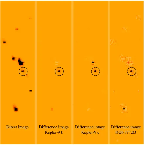
We describe first the use of difference image analysis to demonstrate that the transit sources for all three Kepler-9 planets and candidates are restricted to being very near the target star. A difference image is formed by averaging several exposures near, but outside of a transit and subtracting from this the average of all available exposures near transit center. This results in a typically isolated signal, a positive intensity with the shape of the point-spread function (PSF) at thetrue spatial location of the transit source, and an amplitude equal to the photometric transit depth times the direct image intensity for the target. Adopting 40 independent transits of KOI-377.03 in quarter 3 (avoiding those shortly after major disturbances such as a safing event, and avoiding any that overlap with “b” and “c” transits), each formed with six symmetrically placed exposures outside of transits (after a two exposure gap) and three near transit minimum, results in a 14σ signal in the difference image. The corresponding direct image is formed as the average of both in-and out-of-transit sets such that the direct in-and difference images are sums and differences of precisely the same exposure sets.
For Kepler-9 b four transits were used from quarter 3 with five exposures in transit, a gap of three, then five more exposures on each side for out-of-transit. Kepler-9 c used two transits with seven exposures in-transit, a gap of three, and seven symmetrically placed out-of-transit exposure blocks. By using only exposures pulled close in time, and symmetrically with respect to the transits in use to form a difference image, this effectively imposes a de-trending and avoids any complications from drifts on timescales longer than the average spread of the out-of-transit sets, which for Kepler-9 c (the widest) is about 9 hr. Inspection of the difference images in Figure 3 shows that the transit sources for the confirmed “b” and “c” planets (Holman et al.2010) and the candidate KOI-377.03 must arise from close to the target star, with offsets approaching 1 pixel easily ruled out by inspection. A weighted PSF fit (or more
Direct image Difference image
Kepler-9 b Kepler-9 c Difference image
[image:6.612.321.569.55.303.2]KOI-377.03 Difference image
Figure 3.Direct and difference images for Kepler-9. The four panels from left to right show 128 (row) by 30 (column) regions corresponding to the direct and difference images for planets “b” and “c,” and candidate KOI-377.03. The pixels returned for all stars in this area have been mapped into original row and column locations on the detector. Over 90% of the image area is unfilled sinceKepler returns only postage stamps on stars of interest. The target (KIC 3323887) is indicated with circles in each panel. The locally brightest pixel is always at column 1100 and row 273, and each display panel has been normalized by the sum of counts within the 3×3 pixels centered on [1100, 273]. The display range is−0.03 to 0.3. The difference images were created to isolate the signals for transits “b,” “c,” and 377.03, respectively. Most stars, not having variations synced with these phases, effectively disappear in the difference images. For each of the three sets of transits the difference image in the 3×3 pixel core appears nearly identical to the direct image, demonstrating that the true transit source must be near the target to a small fraction of a pixel. The difference images also reflect the expected count levels for the source to be coincident with the target.
(A color version of this figure is available in the online journal.)
properly, a Pixel Response Function (PRF) fit; see Bryson et al.
2010) to each of the direct and three difference images of Figure
Table 2
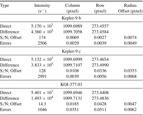
PRF Centroid Measurements on Kepler-9 Direct and Difference Images
Type Intensity Column Row Radius
(e−) (pixel) (pixel) Offset (pixel) Kepler-9 b
Direct 5.170×10⁷ 1099.6989 273.4557 Difference 4.360×10⁵ 1099.7058 273.4584
S/N; Offset 174 0.0069 0.0027 0.0074
Errors 2506 0.0029 0.0039 0.0049
Kepler-9 c
Direct 5.132×10⁷ 1099.6999 273.4654 Difference 3.833×10⁵ 1099.7107 273.4990
S/N; Offset 128 0.0108 0.0336 0.0353
Errors 2991 0.0039 0.0056 0.0068
KOI-377.03
Direct 5.401×10⁷ 1099.6946 273.4408 Difference 1.493×10⁴ 1099.7131 273.4836
S/N; Offset 14.3 0.0185 0.0428 0.0047
Errors 1046 0.0351 0.0511 0.0062
Notes.The first two lines of each block present intensity and two coordinate position PRF fit results for the direct and difference images, respectively. The third line shows the photometric signal-to-noise for the intensity in the difference image, then the offset in position of the preceding two lines, with the last entry being the quadrature sum of the column and row offsets. Errors refer to the PRF fit to the difference image. The scale is 1 pixel=3.98.
98.6% of the area within the 8 pixel optimal aperture (>99.6% of the 31 pixel mask) of Figure1 as the location of potential background eclipsing binaries creating the KOI-377.03 signal.
The quantitative results for all three transit sets are given in Table2. Kepler-9 b shows an offset of 0.0074 pixels between the difference and direct image relative to a 1σ error of 0.0049 pixels. A 3σ error circle in which background binaries cannot be excluded from the centroid analysis ofKeplerdata itself is only 0.06. Kepler-9 c is the only case of the three showing a formal inconsistency with the offset being 5σ; however, even if we combine the offset and 3σ formal error any background eclipsing binaries outside of a radius of 0.22 are excluded as the transit signal source. Clearly for all three transit sets, with the 3σ error circles comfortably under 1, all of the known companions from high-resolution imaging shown in Table1are safely ruled out as sources of the photometric transit signal. It is worth noting that the formal (and equal to scatter from Monte Carlo simulations) error on radial offsets is approximately equal in pixel units to the inverse photometric S/N, as expected (see, e.g., King1983).
Further confirmation that at least the two deeper signals seen in Kepler-9 are not due to known stars in the scene can be obtained by placing simulated eclipses on the known stars in the aperture and comparing them with the observations. The scene in the aperture is modeled using stars in theKeplerInput Catalog (KIC; Latham et al.2005), supplemented by the stars in Table1. All stars within a PRF size (15 pixels) in row or column of Kepler-9’s aperture are included. To generate the modeled out-of-transit image, the measured PRF is placed at each star’s location on the focal plane, scaled by that star’s flux. This provides the contribution of each star to the flux in the aperture’s pixels. For each starsiin the aperture, the depthdsi
of a transit is computed that reproduces the observed depth in the aperture pixels. An in-transit image for eachsiis created as in the out-of-transit image, but with the flux ofsisuppressed by
1−dsi. These model images are subject to errors in the PRF
(Bryson et al.2010), so they will not exactly match the sky. A flux-weighted centroid is computed for the out-of-transit image and the in-transit-image generated for each star in the aperture. This produces row and column centroid offsetsΔR
andΔC, and the centroid offset distanceD=√ΔR2+ΔC2. To compare these modeling results with observation we must make low-noise centroid measurements from the observed pixel data. We do this by creating out-of-transit and in-transit images from de-trended, folded pixel time series. For each pixel time series, the de-trending operation has three steps: (1) removal of a median-filtered time series with a window size equal to the larger of 48 cadences or three times the transit duration, (2) removal of a robust low-order polynomial fit, and (3) the application of a Savitzky–Golay filtered time series of order three with a width of 10 cadences. The Savitzky–Golay filter is not applied within 2 cadences of a transit event, so the transits are preserved. The resulting pixel time series are folded with the transit period. Each pixel in the out-of-transit image is the average of 30 points taken from the folded time series outside the transit, 15 points on either side of the transit event. Each pixel in the in-transit image is the average of as many points in the transit as possible: seven for Kepler-9 b and Kepler-9 c and four for KOI-377.03. Centroids are computed for the in-transit and out-of-transit images in the same way as the modeled images.
Uncertainties of these centroids are estimated via Monte Carlo simulation, where a noise realization is injected into 48 cadence smoothed versions of the pixel time series for each trial. A total of 2000 trials are performed each for Kepler-9 b, Kepler-9 c, and KOI-377.03. The in-transit and out-of-transit images are formed using the same de-trending, folding, and averaging as the flight data. The measured uncertainties are in the range of a few times 10−5pixels.
Table 3 shows the resulting measurements of the cen-troids from quarter 3 pixel data, along with the Monte Carlo based 1σ uncertainties. The centroids are converted into cen-troid offsets and offset distance with propagated uncertainties. Table4shows the offset distanceDpredicted by the modeling method described above for each target in the aperture. We see that when the transit is on Kepler-9 itself we expect a measur-able centroid shift for Kepler-9 b and Kepler-9 c. In this case the modeled centroid shift is about 3.7 times larger than that observed, though the signs of the offsets agree. This exaggera-tion of the centroid offset has been traced to inaccuracies in the KIC used to create the model images. Therefore, the centroid shifts in Table4should be scaled by a factor 1/3.7. If the transit were on one of the companion stars in the aperture, then the modeled centroid shift would be an order of magnitude larger than observed for Kepler-9 b and Kepler-9 c, ruling out the com-panion stars as the source for these signals. Comcom-panion stars are not as definitively ruled out for the KOI-377.03 transit by this technique. After scaling the centroid offsets as above, modeled transits on companions 3 and 4 have offsets that are about 2.5σ, while companion 2 is 1.9σ and companion 1 is less than 1σ. The modeled transit on Kepler-9, however, is much smaller, consistent with the observed transit offset for KOI-377.03.
3.4.BLENDERAnalysis of Kepler-9 b and c
Table 3
Observed Centroid Shifts for Kepler-9 b, Kepler-9 c, and KOI-377.03
Kepler-9 b Kepler-9 c KOI-377.03
ΔR 2.52×10⁻⁴±7.78×10⁻⁵ 1.65×10⁻⁴±9.34×10⁻⁵ −1.24×10⁻⁷±6.19×10⁻⁵
ΔC −2.23×10⁻⁴±7.55×10⁻⁵ −2.40×10⁻⁴±9.21×10⁻⁵ 8.39×10⁻⁶±5.82×10⁻⁵
D 3.41×10⁻⁴±7.66×10⁻⁵ 2.91×10⁻⁴±9.25×10⁻⁵ 8.39×10⁻⁶±5.82×10⁻⁵
D/σ 4.44 3.15 0.14
[image:8.612.118.495.188.257.2]Note.The measurements are given in pixel units, and the scale is 3.98 per pixel.
Table 4
Modeled Centroid Shifts Due to Transits on the Known Stars in the Aperture with Depths that Reproduce the Observed Depth
Object ModeledD D/σ Object ModeledD D/σ Object ModeledD D/σ
Kepler-9 b 1.22×10⁻³ 16.0 Kepler-9 c 1.10×10⁻³ 11.9 KOI-377.03 5.02×10⁻⁵ 0.86 Comp 1 depth>1 . . . Comp 1 depth>1 . . . Comp 1 1.45×10⁻⁴ 2.49 Comp 2 9.77×10⁻³ 127 Comp 2 8.75×10⁻³ 94.6 Comp 2 4.01×10⁻⁴ 6.89
Comp 3 depth>1 . . . Comp 3 depth>1 . . . Comp 3 5.33×10⁻⁴ 9.16
Comp 4 1.44×10⁻² 188 Comp 4 1.29×10⁻² 139 Comp 4 5.90×10⁻⁴ 10.1
Notes.Shifts are given in pixel units, and the scale is 3.98 per pixel. For Kepler-9 b and Kepler-9 c transits on some companions can be ruled out because they require depth>1.
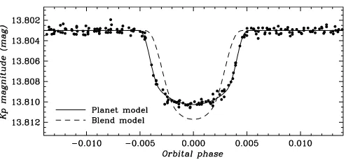
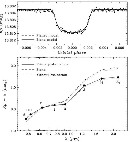
the primary, and corresponds to [Fe/H] =+0.12 and an age of 1 Gyr. The secondary and tertiary masses were allowed to vary freely between 0.10M (the lower limit in the models; see footnote 22) and 1.40M, as mentioned earlier, seeking the best fit to the photometry. The inclination angle was also free, and the orbits were assumed to be circular. In both Kepler-9 b and c, which have similar transit signals, we find that the best-fitting hierarchical triple blend model corresponds to secondaries that are approximately 1.0 and 0.5 mag fainter than the primary, respectively, and tertiaries that are at the lower limit of the isochrone range (late M dwarfs). However, these fits give a poor match to the photometry:BLENDERis unable to simultaneously reproduce the total duration of the transit and the central depth, given the constraints on the brightness and size of the stars from the isochrones. This type of blend scenario is therefore clearly ruled out. We illustrate this for Kepler-9 b in Figure 4, where the best-fit planet model is also shown for reference. Much better matches to the data can be found if additional light from a fourth star along the line of sight is incorporated into the model, providing extra dilution. We find that this fourth star is required to be nearly as bright as the primary, and the optimal model changes in such a way that the secondary also becomes as bright as the primary (so that its size enables the duration of the transits to be reproduced), while the tertiary remains a small star. This rather contrived scenario requiring two bright stars that are nearly identical to the main star would be easily recognized in our high-resolution imaging for separations larger than about 0.1 (see, e.g., Figure 2), in our centroid analysis for separations larger than 0.06, or would otherwise produce obvious spectroscopic signatures unless all three bright objects happened to have the same radial velocity.
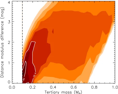
[image:8.612.321.568.297.411.2]We next considered blends involving eclipsing binaries in the background, by removing the constraint on the distance. In this case a solar-metallicity isochrone was adopted for the binary, with a representative age for the field of 3 Gyr. We explored a wide range of relative distances, and we first considered main-sequence stars only, again with circular binary orbits. The results for Kepler-9 b and c are once again similar to each other, and we illustrate them for Kepler-9 c in Figure5. The axes correspond to the distance modulus differenceΔδas a function of the tertiary mass. Contours represent constant differences in theχ2of the
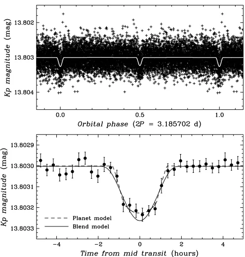
Figure 4.Light curve of Kepler-9 b (P=19.24 days) with the best-fit blend model for the case of a hierarchical triple (candidate + physically associated eclipsing binary). The best-fit planet model is shown for reference. The poor fit of the blend model rules out this configuration.
fit compared to the best-fit planet model and are labeled in units of the statistical significance of the difference (σ). We draw two main results from this figure. One is that the light curve fits strongly prefer the smallest available tertiary masses from the isochrones (0.10 M), and would in fact yield better fits for even smaller tertiaries (i.e., planets). Additionally, the best solutions cluster toward equal distances for the binary and the primary star, effectively converging toward the equivalent of the hierarchical triple scenario considered earlier. No acceptable solutions exist with the binary at a significant distance behind the primary star. The best fit to the light curve of Kepler-9 c is similar to the one shown in Figure4(dashed curve), which is not particularly good. TheΔδversus tertiary mass diagram for Kepler-9 b is qualitatively the same. Allowing the secondary to be a giant star gives a very poor fit to the photometry: the duration of the transit is very much longer than observed, there is out-of-eclipse modulation due to distortions in the giant, and all solutions place the binary at an implausibly large distance. We conclude that blend configurations involving background eclipsing binaries in which the tertiary is a star are not a viable explanation for either of these two signals.
Figure 5.Map of theχ2surface (goodness of fit) corresponding to a grid of blend models for Kepler-9 c (P=38.91 days) involving background eclipsing binaries with circular orbits. The separation between the binary and the primary is expressed in terms of the distance modulus difference. Contours are labeled with theχ2difference from the best planet model fit (expressed in units of the
significance level of the difference,σ) and are plotted here as a function of the mass of the tertiary star. The dashed line at 0.1Mindicates the lower limit to the tertiary mass set by the model isochrones we use.
(A color version of this figure is available in the online journal.)
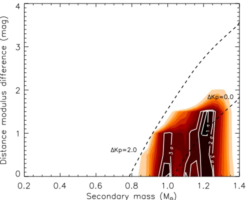
Figure 6 shows the results for Kepler-9 c, this time in the plane of separation versus secondary mass. Once again the fits tend to favor an equal distance for the binary and the primary star, and background scenarios with the binary far behind provide unacceptably poor matches to the light curve. A second noteworthy result is that these solutions have a strong preference for secondary stars that are quite similar to the primary. All acceptable fits to the light curve correspond to relatively bright secondaries withΔKp <1.5 mag (see Figure6). The best of these solutions is of about the same quality as a planet model and has a secondary of mass 0.98Mthat is only 100 K cooler and 0.3 mag fainter than the primary in theKeplerband. This somewhat artificial case of “twin” stars is a result we have seen often in simulations for otherKepler candidates. The tertiary in this type of blend solution comes out about√2 larger than in a planet model because the transit is diluted by another star of approximately equal size and brightness. One may debate whether this situation should actually be referred to as a “false positive” for Kepler-9, since the signal would still correspond to a gas giant planet, only that this planet would be√2 larger, and it would be orbiting a different star. Alternatively, it could be thought of simply as an overlooked dilution factor in a true planetary system. In any event, the lack of evidence for this bright twin star in the spectroscopy or in our high-resolution imaging or centroid analysis for Kepler-9 does not support this scenario.
[image:9.612.45.292.55.253.2]As a particular case of this family of configurations, we examined blends in which the star–planet pair is constrained to be at the same distance as the primary, i.e., effectively in a hierarchical system. The secondary properties were therefore taken from the same isochrone as the primary, and the orbits were assumed to be circular. An excellent fit to the light curve is possible for a tertiary that is about√2 larger than in a true planet model, but not surprisingly, we find once more that the secondary must be as bright as the primary.
Figure 6.Map of theχ2 surface corresponding to a grid of blend models
for Kepler-9 c involving background eclipsing systems in which the tertiary is a (dark) planet, in a circular orbit around the secondary. Contours are labeled with theχ2 difference from the best-planet model fit (expressed in
units of the significance level of the difference,σ). Two dashed lines of equal magnitude difference (ΔKp) are indicated and show that all viable blend fits (with confidence level<3σ) have secondaries that are bright enough to have been detected spectroscopically (ΔKp <2).
(A color version of this figure is available in the online journal.)
Additional tests were run to examine the impact of changing the age adopted for the isochrone of the secondary in a background star–planet pair or the addition of light from a fourth object in the aperture. In the first case, changing the age from 3 Gyr to 1 Gyr produced a small shift of the contours in Figure6downward and to the right that is simply due to the change in intrinsic brightness of the secondary star, and does not alter our conclusions. Adding “fourth light” further attenuates the eclipses of the star–planet pair. To compensate, BLENDER
requires a slightly deeper eclipse, and in order to preserve the shape of the signal (total duration, and slope of ingress/egress), this is achieved by bringing the secondary closer to the primary. As a result, for relatively bright fourth light the contours are shifted downward by approximately the difference in magnitude between the primary and the fourth star, again without changing the conclusions.
Figure 7.Top: light curve of Kepler-9 c with the best-fit blend model for the case of contamination by a foreground eclipsing pair with a circular orbit in which the tertiary is a planet. The pair consists of an M2 dwarf (0.56M, 0.58R) and a 0.91RJupcompanion 450 pc in front of the primary, which is at 750 pc.
This fit is statistically indistinguishable from best-fit planet model, also shown for reference. Bottom: measured colors for Kepler-9 (dots) compared with the predictions from the blend model in the top panel. A small amount of extinction (0.15 mag kpc−1) has been included in these predictions. The results without
considering extinction differ little and are shown with dotted lines. The color measurements clearly rule out such a blend.
foreground secondaries, which necessarily involve later-type stars. We find that of these, the only ones that yield acceptably good fits to the Kepler photometry, with χ2 values differing from the planet fit by less than 3σ, correspond to secondaries that are within about 1.5 mag of the primary in brightness, and are of course redder. These would be valid blend configurations so long as the secondaries are close enough to the primary to be spatially unresolved (angular separations0.1), and at the same time faint enough to have gone undetected in the spectra. Stars that are within∼2–2.5 mag of the primary would generally have been seen spectroscopically, as indicated in Section3.2, and this would exclude these remaining foreground blend configurations. Nevertheless, to be conservative, let us assume for the moment that a star 1.5 mag fainter than the primary has still managed to elude detection in our spectra. This corresponds to the faintest secondary in a foreground blend scenario that still allows for a satisfactory fit to the light curve, and would be the most difficult case of this kind to disprove. This fit is shown in the top panel of Figure7and is statistically indistinguishable from a planet model fit. The secondary in this configuration is an M2 dwarf (M=0.56M) 1.53 mag fainter than the primary, eclipsed by a 0.91RJupplanetary companion, and is located at a distance of 300 pc. The primary in this scenario is at 750 pc.
[image:10.612.322.569.53.373.2]Other properties of this particular blend such as magnitudes and colors can be computed easily withBLENDER, and compared with observations. Apparent magnitudes for Kepler-9 are avail-able from the KIC for a variety of passbands including Sloan
Figure 8.Effect of eccentricity on the duration of transits relative to the circular orbit case (Δ/Δcirc), on the impact parameter (b/bcirc), and on the displacement
(φsec−0.5) of the secondary eclipses relative to phase 0.5, all shown as a function of the longitude of periastronω. The different curves correspond to eccentricities from 0.1 to 0.7 in steps of 0.1.
griz, a special-purpose passband referred to as D51 (centered on the Mgib triplet at 518.7 nm), andJHKsfrom the 2MASS
catalog. The lower panel of Figure7shows various color indices (Kp−λ) predicted byBLENDERboth for the primary star alone and for the blend. Those of the primary are well reproduced by the model, and we find that a small amount of interstellar ex-tinction leads to an even better match (solid line in the figure). The colors of the blend, on the other hand, disagree with the measured colors and deviate by more than 0.4 mag for the red-dest index,Kp−Ks. We are therefore able to exclude, solely on the basis of its color, this most difficult of the scenarios involv-ing foreground star–planet pairs that could mimic the 19 day and 39 day signals in the light curve of Kepler-9. Larger-mass secondaries would not be as red and still allow for good fits to the photometry, but they are intrinsically brighter and would be recognized more easily.
Figure 9.Same as Figure6(Kepler-9 c), restricted to star–planet orbits having
e=0.3 (concentration of contours on the left) and 0.5 (right), andω=90◦. This orientation corresponds to transits that occur at periastron. Comparison with Figure6shows that these solutions allow for more massive (larger) secondary stars than in the case of circular orbits, but the brightness of these blends is still within 2 mag of the target, and is ruled out by spectroscopy.
(A color version of this figure is available in the online journal.)
a fixed (measured) duration, eccentric orbits may allow blends with smaller or larger secondary stars than in the circular case to still provide satisfactory fits to the light curve, effectively increasing the pool of potential false positives. The limiting cases correspond toω = 90◦ and 270◦, in which the line of apsides is aligned with the line of sight and the transit occurs at periastron (accommodating larger secondaries) or apastron (smaller secondaries), respectively. Extensive simulations for these two extreme situations show that allowing for eccentric orbits does not change our conclusions regarding hierarchical triple systems, background eclipsing binaries, or background star–planet scenarios. We show this for the latter blend category in Figure9, illustrated for the case of orbits with eccentricities of 0.3 and 0.5, andω=90◦. Comparison with Figure6indicates that in both cases the blends are still bright enough that we would have seen signatures of them in the spectra of Kepler-9. Larger eccentricities ofe=0.7 result in secondaries that are brighter still. For eccentric orbits oriented such that transits take place at apastron (ω=270◦), we only find acceptable fits to the light curves for eclipsing star–planet pairs that are in the foreground (and involve smaller stars). However, as was the case for circular orbits, those blends are either too bright, too red, or both, and are thus also excluded.
The above, fairly exhaustive exploration of parameter space withBLENDERallows us to conclude that no configuration in-volving an eclipsing binary (or an eclipsing star–planet pair), either in the foreground or in the background, is able to provide a reasonable explanation for the signals of Kepler-9 b and c (see Table5for a summary of the configurations tested and the re-sults). Many scenarios lead to light curves that match the detailed shape of the transit events, but none are simultaneously consis-tent with all of the other observational constraints. This includes spectroscopy, high-resolution imaging, centroid measurements, and photometry (colors). Therefore, even ignoring the evidence from TTVs, these results fully support the planetary nature of these objects and demonstrate the usefulness ofBLENDER for validating transiting planet candidates fromKepler.
3.5.BLENDERAnalysis of KOI-377.03
We proceed next to examine false positive scenarios for the shallowest signal in Kepler-9, withP =1.59 days, which would correspond to a super-Earth-size planet. Because the period is so short in this case, and tidal forces in such binary systems have likely circularized the orbit (see, e.g., Mazeh 2008 and references therein), we do not consider non-zero eccentricities. Additionally, blends in which the secondary star is a giant need not be considered, as those cases are obviously ruled out because of the short orbital period and small implied semimajor axis of the orbit.
As for the larger signals considered above, hierarchical triple systems in which the tertiary is a star fail to provide good fits to KOI-377.03. A good match to the Kepler photometry can be found when the tertiary is allowed to be a much smaller object (i.e., a planet), but as was the case earlier, it requires a secondary that is very similar to the primary in brightness. The resulting size of the eclipsing object is√2 larger than in a planet model or slightly over 2R⊕. This type of configuration was ruled out earlier based on the high-resolution imaging and the spectroscopy. Small tertiaries with appreciable mass, such as white dwarfs, induce tidal distortions on the primary due to the short orbital period that lead to significant out-of-eclipse variations in the light curve (ellipsoidal variability). These modulations are not seen in the photometry for Kepler-9, and such false positives are therefore also excluded.
Table 5
Summary of Blend Configurations Tested for Kepler-9 b and c
False Positive Configurationa Result Blends Ruled Out
Hierarchical triple with stellar tertiary, MS
Circular and eccentric orbits Poor fits/sec. ecl. Yes
Added fourth light Twin star Yes (imaging/spec./centr.)
Hierarchical triple with planetary tertiary, MS
Circular and eccentric orbits Twin star Yes (imaging/spec./centr.)
Background EB with stellar tertiary
Circular and eccentric orbits, MS and giants Poor fits Yes
Background EB with planetary tertiary, MS
Circular and eccentric orbits Twin star Yes (imaging/spec./centr.)
1 Gyr isochrone for secondary Little change Yes (imaging/spec./centr.)
Added fourth light Little change Yes (imaging/spec./centr.)
Foreground EB with stellar tertiary, MS
Circular and eccentric orbits Poor fits/sec. ecl. Yes
Foreground EB with planetary tertiary, MS
Circular and eccentric orbits Too bright/Too red Yes (imaging/spec./centr./color)
Note.
a3 Gyr isochrone and solar metallicity assumed for background and foreground stars, unless otherwise indicated.
[image:12.612.46.289.307.503.2]Abbreviations: MS, main-sequence secondary; imaging/spec./centr., high-resolution imaging, spectroscopy, and centroid analysis; sec.ecl., secondary eclipses predicted but not observed; EB, eclipsing binary.
Figure 10.Map of theχ2surface for KOI-377.03 corresponding to a grid of
blend models involving background eclipsing binaries with stellar tertiaries. Contours are labeled with theχ2 difference from the best planet model fit
(expressed in units of the significance level of the difference,σ). The dashed lines indicate levels of equal apparent magnitude differenceΔKpbetween the background binary and the primary star.
(A color version of this figure is available in the online journal.)
[image:12.612.319.565.308.505.2]Figure 11.Example of a blend model fit to KOI-377.03 involving a background eclipsing binary with a stellar tertiary (solid line). The secondary is similar in spectral type to the primary and 5.2 mag dimmer, and the tertiary is a late M dwarf. The eclipsing pair is 6 kpc behind the primary. This fit is statistically indistinguishable from the best-fit planet model, which is shown with a dashed line. TheKeplerobservations have been binned for clarity.
Figure 12.Same as Figure10, including the effect of differential extinction in the amount of 0.5 mag kpc−1. The net effect of extinction is to compress and
shift the contours toward smaller relative distances. The dashed lines indicate levels of equal apparent magnitude differenceΔKpbetween the background binary and the primary star and are the same as shown in Figure10.
(A color version of this figure is available in the online journal.)
In the above calculations we have ignored interstellar ex-tinction. However, given the large distances for the binaries in some of these blend configurations, it is worth exploring the effect of dust more carefully, which we have done by repeat-ing theBLENDERsimulations using a representative differential extinction coefficient of 0.5 mag kpc−1. The results are shown in Figure 12 and indicate that the blend scenarios providing good fits to theKeplerphotometry of KOI-377.03 are system-atically shifted to smaller distances compared to the previous calculations. Their apparent brightness, however, changes rel-atively little, as can be seen by comparing the lines of equal
[image:12.612.43.295.581.690.2]Figure 13.Same as Figure12, but for the case in which the tertiary is a planet instead of a star. Differential extinction is included. Kinks in the contours are an artifact of the discreteness of our grid. The dashed lines indicate levels of equal apparent magnitude differenceΔKpbetween the background secondary and the primary star. The lower of these lines represents the constraint from the spectroscopy for Kepler-9 (see the text).
(A color version of this figure is available in the online journal.)
Allowing the tertiary to be a smaller object such as a planet opens up a different area of parameter space for permissible background blends (Figure13). When including extinction as before, acceptable fits to the light curve are possible for Δδ
values from zero up to about 4.5. This upper limit corresponds to distances for the star–planet pair of about 4.8 kpc (with
ΔKp≈6, or apparent magnitudes ofKp≈20) and is set by the maximum size of 1.8RJupwe have allowed for a planet. As in the configurations described before, the solutions constrain the secondary masses to be near that of the primary in order to match the detailed shape and observed duration of the transits, with a range from about 0.9Mto 1.2M. Therefore, the color of the blend is not as useful a discriminant in this case. Secondaries that are less than about 2 mag fainter than the primary would have been seen spectroscopically. This excludes a good fraction of the space of parameters, as indicated by the lower dashed line in Figure13. Of the remaining blends of this kind between
ΔKp=2 andΔKp=6, only the ones with angular separations smaller than about 1 are allowed by the constraints from our AO imaging (see Figure2), but the centroid analysis is even more restrictive and rules out stars outside of 0.74. At closer separations, the high-resolution images rule out all blends that are brighter than the sensitivity limit indicated in Figure2(i.e., those that fall above the curves).
[image:13.612.319.568.54.258.2]As expected from the fixed duration and depth of the transit-like signal of KOI-377.03, the size of the tertiary in these configurations correlates with the secondary mass. Due to this correlation, small tertiaries with R 0.3RJup (roughly Neptune-size and smaller) are further excluded because the eclipses they produce are already very shallow, and further dilution by the primary would make them too shallow to fit the photometry. In order to avoid this, the secondaries in those blends must be relatively small late-G type stars that are nearby, and would therefore be bright enough (ΔKp 2) that they would have been detected in our spectra as a second set of lines. Thus,BLENDEReffectively places limits not only on the secondary, but also on the size of the tertiary (see Figure14).
Figure 14.Same as Figure13, shown here as a function of the tertiary radius. Kinks in the contours and closed inner contours for the 1σ and 2σ levels are an artifact of the discreteness of our grid. We indicate with a dashed line the lower limit for the size of the tertiaries that is set by the spectroscopic constraint on presence of bright stellar companions (see the text). The sizes of the Earth, Neptune, and Saturn are also indicated for reference.
(A color version of this figure is available in the online journal.)
In particular, blends with a white dwarf eclipsing a background star are also ruled out for the same reason described above. Additionally, the predicted light curves for such cases with white dwarf tertiaries show ellipsoidal variability, which is not observed.26Many of the larger tertiaries correspond to gas giants (Saturn-size or larger), which implies a qualitative difference in their nature compared to the alternate model of a true Earth- or super-Earth-size planet. In this sense these blends may properly be considered “false positives,” as opposed to the configurations discussed earlier requiring twin stars, which only change the tertiary radius by√2.
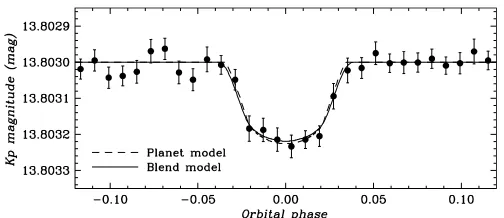
Finally, we examine the possibility that the true period of the KOI-377.03 signal is twice the nominal value. Alternating events would then correspond to the primary and secondary eclipses of a blended eclipsing binary (the tertiary being a star in this case), which may in general be of different depth. In KOI-377.03 there is no compelling evidence for a depth difference between odd- and even-numbered events, but this is difficult to establish in a faint star such as this for a signal that is only 0.2 mmag deep. The results of extensive simulations with
BLENDERfor this scenario are illustrated in Figure15. The best fits correspond to blended binaries far in the background, and do not indicate a significant difference in depth between the primary and secondary eclipses. However, these fits provide only a poor representation of theKeplerlight curve, and can therefore be confidently ruled out. This is seen in Figure16. The top panel shows the closest fit to the full light curve together with the data, and in the bottom panel we have binned the measurements to facilitate the comparison. This solution involves an eclipsing
26 We note, for completeness, that the mass of a white dwarf would generally
also be sufficient to induce tidal synchronization in the secondary star, resulting in line broadening that could in principle render it more difficult to detect in the spectrum. However, given the orbital period and typical secondary sizes allowed byBLENDER, we estimate the rotational broadening to be no more than∼30 km s−1, which should still allow that star to be seen