Rochester Institute of Technology
RIT Scholar Works
Theses
7-26-2019
Prediction of Treatment Target for Ventricular
Tachycardia using Multi-Task Machine Learning
Vishwanath Raman
Follow this and additional works at:
https://scholarworks.rit.edu/theses
This Thesis is brought to you for free and open access by RIT Scholar Works. It has been accepted for inclusion in Theses by an authorized
Recommended Citation
Prediction of Treatment Target for Ventricular
Tachycardia using Multi-Task Machine Learning
by
Vishwanath Raman
A Thesis Submitted to the
B. Thomas Golisano College of Computing and Information
Sciences Department of Computer Science
in partial fulfillment of the requirements for the degree of
Master of Science in Computer Science
at Rochester Institute of Technology
Committee Approval
Linwei Wang
Date
Thesis Advisor
Richard Zanibbi
Date
Reader
Joe Geigel
Date
Abstract
Acknowledgements
First and foremost I wish to thank my advisor Dr. Linwei Wang for giving me an opportunity to pursue research in her lab during the start of my masters journey. Without her help I could not have overcome the obstacles (of which there were many) to achieve my dream of pursuing a thesis. I am forever grate-ful for the experience I gained working with her, in research and in computer science.
I would like to thank Dr. Richard Zanibbi for his meticulous feedback for my thesis and inspiring me to delve into machine learning through his introductory machine learning course; It was without a doubt the most fun learning experi-ence I have had in an academic course. I am thankful to Dr. Joe Geigel for his time and expertise which helped improve my programming knowledge and gave me my first break in the industry.
Due to unavoidable circumstances I struggled with my studies for a couple years and wish to thank my good friend Ameya Lonkar, my academic advisor Cindy Wolfer, and counsellor Brittany Bowhall for helping me get through it. I wish to thank Abishai Dmello for his valuable feedback for my thesis defense and Ryan Missel for his help with my experiments. A shout-out goes to the many people I met at RIT through the Juggling Club, Rock Climbing Club, Swim Club and RITSMA that kept life interesting.
Contents
1 Introduction 1
1.1 Problem Statement and Research Contribution . . . 1
2 Background and Related Works 4 2.1 Cardiac Electrophysiology . . . 4
2.1.1 Anatomy of the Human Heart . . . 4
2.1.2 Cardiac Conduction System and Electrophysiology . . . . 5
2.1.3 Ventricular Tachycardia . . . 7
2.1.4 The Electrocardiogram . . . 7
2.2 Machine Learning . . . 12
2.2.1 Machine Learning in Localizing the Origin of VT . . . 12
2.2.2 Multi-Task Learning . . . 13
3 Methodology 15 3.1 MTL-Based Prediction of VT Origin . . . 15
3.1.1 Predictor Variable . . . 15
3.1.2 Dependent Variable . . . 15
3.1.3 Models . . . 16
3.1.4 Optimization Method . . . 19
4 Experiments and Results 21 4.1 Experimental Data . . . 21
4.2 Results . . . 22
4.2.1 Effect of Grouping Size on Patients . . . 23
4.2.2 The Effect of the Size of Training Data . . . 26
List of Figures
2.1 Chambers of the heart . . . 5 2.2 Ventricular potential.1 . . . . 6
2.3 Conduction system of the heart.1 . . . . 6
2.4 12 different angles of ECG through lead placement in the vertical (blue) and horizontal (red) plane.1 . . . 8 2.5 Correct possible placements of limb electrodes is shown.1 . . . . 9 2.6 Placement of the precordial or chest electrodes is depicted.1 . . . 10 2.7 Limb leads and augmented limb leads.1 . . . 11 2.8 A normal ECG through Lead II. . . 12 4.1 All 12-Leads of ECG for one pacing site plotted together and
annotated. The black lines denote the onset/start of QRS and the green lines denote the offset/end. . . 22 4.2 All the pacing sites for every patient. . . 22 4.3 Error per patient for three different grouping sizes from patient
1 to 13. . . 23 4.4 Error per patient for three different grouping sizes from patient
14 to 26. . . 24 4.5 Error per patient for three different grouping sizes from patient
27 to 39. . . 24 4.6 Two perspectives for prediction of the second pacing site for
pa-tient number 5. The predictions for all three grouping settings overlap as they are very similar. . . 25 4.7 The prediction accuracy for different grouping sizes across all
patients . . . 25 4.8 Prediction accuracy for different group sizes across patients, using
Chapter 1
Introduction
Ventricular tachycardia (VT) is a type of irregular and fast heart rate that arises from improper electrical activity in the ventricles of the heart. This abnormal and fast rhythm from the ventricle may impair the ability of the heart to supply blood to the brain and the rest of the body. As a result, sustained VT is a major cause of many out-of-hospital sudden deaths that occur annually in the US.2
Most VTs involve an abnormal origin of electrical activation inside the ven-tricles. An effective way to treat VT is catheter ablation, which destroys the culprit myocardial tissue serving as the origin of VT by radiofrequency energy.2 To locate this treatment target, it is widely accepted that the origin of ven-tricular activation can be largely determined from the morphology of 12-lead electrocardigram (ECG) signals. To do so, current clinical practice requires a pace-mapping procedure that involves artificial electrical stimulation (i.e. pac-ing) at multiple sites of the heart, until locating the site where pacing reproduces the ECG morphology of the VT.
This however is a trial-and-error method which can take a lot of time and effort. A data-driven prediction model using machine learning can be built to directly predict the origin of ventricular activation using the information from the ECG data. Such a model has the potential to largely reduce the time needed and improve the accuracy for localizing the treatment target for VT.
1.1
Problem Statement and Research
Contribu-tion
How-ever, there are limited investigations that exploit the power of machine learning to predict the origin site of VT using this information. Existing studies have used support vector machines and template matching to localize the origin site, but their accuracy did not meet clinical needs.4, 5 One primary challenge arises from the fact that ECG signals exhibit diversity across individuals due to factors such as the size and orientation of the heart, position of the reference electrodes used to measure ECG, or scar characteristics in patients with structural ab-normality in the heart. Therefore, although a population allow us to learn from multiple patients and predict on an unseen patient, it has fallen short of satisfying the required accuracy in a clinical setting.
A patient-specific model, where we train and test using a single patient’s data, is a potential alternative to avoid the challenge of inter-subject variations. How-ever, it will require a lot of pace-mapping data on that patient. This is im-practical for clinical use, and defeat the purpose of the prediction model to avoid the excessive trial-and-error collection of paced ECG data on the same patient.
To bridge this gap, in this thesis research, we investigate the feasibility of using multi-task learning (MTL) to address the challenge of inter-subject variations. We propose to treat the predictive modeling of each subject as a separate task, but assume that these tasks have shared characteristics. In this way, we ask all the subject-specific models to share information, while allowing individual adjustment to the model specific to each patient. Furthermore, while traditional MTL often assumes that all tasks under consideration share something in com-mon, it may not necessarily apply in our application of interest. Rather, it may be more appropriate to assume that the characteristics of given patients can be clustered into several groups. This grouping, however, is not known a priori. This thesis therefore answers the following two research questions:
1. Whether treating subject-specific predictive modeling of VT origin as sep-arate but related tasks, in comparison to independent subject-specific modeling, may improve the accuracy of the models?
2. Whether considering with which patients to share information, rather than assuming all patient-specific models have shared components, will further improve the accuracy of predicting VT origins?
To answer these questions, we adopted a MTL approach proposed by Kang et al.6 which allowed simultaneous optimization of task grouping and MTL within
each group for 12-lead ECG based prediction of VT origin. When the number of groups is equal to one or the total number of tasks, this approach is respectively reduced to a standard MTL approach forcing all tasks to share information as reported by Argyriou et al.7 and a standard independent patient-specific
Chapter 2
Background and Related
Works
2.1
Cardiac Electrophysiology
2.1.1
Anatomy of the Human Heart
The human cardiovascular system is responsible for circulating blood through-out the human body to supply tissues with oxygen and nutrients. The heart is located in the mediasternum, a region that extends from the sternum (breast-bone) to the vertebral column in the dorsoventral aspect, from the first rib to the diaphragm in the anterio-posterior aspect, and between the lungs.
It consists of four chambers (Figure 2.1):
• Two superior receiving chambers called atria (left and right), which receive blood coming back to the heart from all over the body.
• Two inferior pumping chambers called ventricles (left and right) that pump blood out of the heart for supply to all parts of the body.
Figure 2.1: Chambers of the heart
2.1.2
Cardiac Conduction System and Electrophysiology
The heart is made up of cardiac muscle tissue which gives it its contractile abil-ity in response to an electrical stimulus. Special structures in the cardiac muscle tissue called gap junctions enable it to conduct electrical signals to neighboring fibers, and the atria and ventricles, to contract as a single coordinated unit. The electrical stimulus for a contraction is called the cardiac action potential. Normal contractile muscle fibers - or muscle cells - typically have a stable resting membrane potential of around -90mV (or are ‘polarized’), which is maintained by the cell membrane that contains gated ion channels to restrict the flow of ions in and out of the cells. This makes the cells responsive to any change in ionic concentration, i.e., an electrical stimulus, and hence the ability to conduct electrical signals. When their neighboring cells reach a potential over the thresh-old at -40mV, they will go through a rapid depolarization (-90mV to 10mV), followed by repolarization (10mV to -90 mV). A typical ventricular contractile fiber action potential is given in Figure 2.2. An atrial contractile fiber action potential is similar except for the time intervals of each phase.
The action potential propagates through the heart in the following manner (Figure 2.3):
• The excitatory stimulus begins in a small bundle of autorhythmic fibers called the sinoatrial node (SA node) located in the right atrial wall. The SA node is also called the pacemaker of the heart. These cells do not have a stable resting membrane potential, but rather repeatedly ‘depolarize’or undergo a rise in their membrane potential spontaneously. This is then propagated to the contractile cardiac muscle fibers throughout both atria. This first phase of conduction where the atria contract is known as atrial depolarization.
Figure 2.2: Ventricular potential.1
Figure 2.3: Conduction system of the heart.1
another mass of autorhythmic fibers known as theatrioventricular (AV) nodelocated in the interatrialseptum. At the AV node, the action poten-tial slows considerably as a result of various differences in cell structure in the AV node. It acts as an important delay in the conduction system providing time for the atria to contract fully and to empty their blood into the ventricles.
branches are many specialized conducting fibers, called Purkinje fibers, that carry the signal to the walls of the ventricles. These fibers allow the conduction system of the heart to create synchronized contractions of the ventricles and are a vital part of maintaining normal heart rhythm. The ventricular contractile muscle fibers are stimulated by the Purkinje fibers to undergo a cardiac action potential and this is when both the ventricles undergo depolarization and hence ventricular contraction.
After this, the cardiac muscle fibers of the ventricles repolarize (ventric-ular repolarization) to prepare for the next round of depolarization and contraction.
2.1.3
Ventricular Tachycardia
VT occurs most commonly in patients with weakened heart muscle (cardiomy-opathy) or when scar tissue develops in the heart. In patients with coronary artery disease (blockage of blood vessels on the surface of the heart), this scar is the result of a prior heart attack (myocardial infarction) when the muscle dies as a result of a blockage in blood flow. Scar, or fibrosis, can interfere with the con-duction of a normal electrical impulse in the heart, leading to a short-circuiting of the impulse, called reentry. VT can also occur in patients with normal hearts by a different mechanism whereby the electric conduction is overly excitable, like a muscle twitch. However, the majority of VT cases involve a channel formed in a region of myocardial scar, which creates a pathway for reentry of the electrical impulse and in turn causes the ventricles to contract prematurely.2
Catheter ablation, is a minimally-invasive procedure used to remove or termi-nate a faulty electrical pathway from sections of the hearts. It has been used to treat heart rhythm disorders for more than 25 years. The procedure targets the origin of the VT by placing a long, thin wire or catheter into the heart chambers through the veins of the leg. When areas that result in the generation of the faulty electrical pathway are identified, a localized delivery of radiofrequency energy is applied, which produces a small burn about 5 to 10 mm in diameter and thus ablates that site. For VT, ablation targets the origin of the short circuits, i.e., the origin of the ventricular activation that forms the short circuit.
2.1.4
The Electrocardiogram
Figure 2.4: 12 different angles of ECG through lead placement in the vertical (blue) and horizontal (red) plane.1
The most common way of recording an ECG waveform is the conventional 12-lead ECG where 10 electrodes are placed, four on the patient’s arms and legs and six on the surface of the chest. An electrode is a conductive pad in contact with the body that makes an electrical circuit with the electrocardiograph while a lead is a connector to an electrode. Hence leads can share the same electrode and the electrocardiograph produces 12 different tracings from different combinations of limb and chest leads. Each limb and chest electrode records slightly different electrical activity because of the difference in its position relative to the heart. By comparing these records with one another and with normal records, it is possible to detect any abnormalities in the conduction pathway. A 12-lead ECG thus paints a complete picture of the heart’s electrical activity by recording information through 12 different angles through two electrical planes - vertical and horizontal planes over a period of 10 seconds (Figure 2.4). In this way, the overall magnitude and direction of the heart’s electrical depolarization is captured at each moment throughout the cardiac cycle. The output of this noninvasive medical procedure is a graph of voltage versus time.
The 10 electrodes in a 12-lead ECG consisting of four limb and six precordial electrodes are listed below:
• RA - One the right arm, avoiding thick muscle.
• LA - In the same location where RA was placed but on the left arm.
• RL - One the right leg, lower end of medial aspect of calf muscle.
• LL - In the same location where RL was placed, but on the left leg.
Figure 2.5: Correct possible placements of limb electrodes is shown.1
of the sternum.
• V2 - In the fourth intercostal space, between ribs 4 and 5, just to the left
of the sternum.
• V3- Between leads V2 and V4.
• V4 - In the fifth intercostal space, between ribs 5 and 6, in the
mid-clavicular line.
• V5- Horizontally even with V4, in the left anterior axillary line.
• V6- Horizontally even with V4 and V5 in the midaxillary line.
The placement of the limb electrodes and the precordial electrodes can be seen in figure 2.5 and Figure 2.6 respectively. In a 12-lead ECG, the Wilson’s central terminal VW is produced by averaging the measurements from the electrodes RA, LA, and LL to give an average potential across the body.
VW =
1
3(RA+LA+LL)
There are two electrical planes that are utilized for lead placement:
Frontal leads (vertical plane): By using 4 limb electrodes, one can get 6 frontal leads that provide information about the heart’s vertical plane (Figure 2.7). These are:
Figure 2.6: Placement of the precordial or chest electrodes is depicted.1
I=LA−RA
2. Lead II is the voltage between the (positive) left leg (LL) electrode and the right arm (RA) electrode.
II =LL−RA
3. Lead III is the voltage between the (positive) left leg (LL) electrode and the left arm (LA) electrode.
III=LL−LA
4. Lead augmented vector right (aVR) has the positive electrode on the right arm. The negative pole is a combination of the left arm electrode and the left leg electrode.
aV R=RA−1
2(LA+LL) = 3
2(RA−V W)
5. Lead augmented vector left (aVL) has the positive electrode on the left arm. The negative pole is a combination of the right arm electrode and the left leg electrode.
aV L=LA−1
2(RA+LL) = 3
Figure 2.7: Limb leads and augmented limb leads.1
6. Lead augmented vector foot (aVF) has the positive electrode on the left leg. The negative pole is a combination of the right arm electrode and the left arm electrode.
aV F =LL−1
2(RA+LA) = 3
2(LL−V W)
The limb leads (I, II, and III) and the augmented limb leads (aVR, aVL, and aVF) form the basis of the hexaxial reference system.
Precordial leads: The precordial leads or V leads, V1, V2, V3, V4, V5, V6, lie in the transverse (horizontal) plane, perpendicular to the other six leads. The six precordial electrodes act as the positive poles for the six corresponding precordial leads.
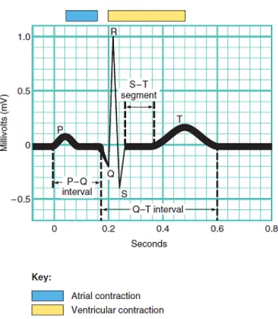
In a typical ECG, three general waves appear with each heartbeat (Figure 2.8).
• P wave: The P wave is a small upward deflection on the ECG. The P wave representsatrial depolarization, which arises in the SA node and spreads through contractile fibers in both atria. After the P wave begins, the atria contract. During the plateau period of steady depolarization,the ECG tracing is flat.
• QRS Complex: The second wave, called the QRS complex, represents
Figure 2.8: A normal ECG through Lead II.
shortly after the QRS complex appears and continues in the S-T segment. At the same time, atrial repolarization is occurring, but it is not usually evident in an ECG because the larger QRS complex masks it.
• T wave: The third wave is called the T wave. It indicates ventricular repolarizationand occurs just as the ventricles are starting to relax. The T wave is smaller and wider than the QRS complex because repolarization occurs more slowly than depolarization.
In reading an ECG, the amplitude of the waves and time intervals between the occurrence of the waves can provide clues to abnormalities.
2.2
Machine Learning
2.2.1
Machine Learning in Localizing the Origin of VT
The QRS complex in an ECG waveform contains important information regard-ing the electrical activity of the ventricles of a human heart. Yokokawa et al.4
showed that the 12-Lead ECG had enough information to help identify a region of interest 10-20 cm2 in size, which contained the origin of VT. Sapp et al.5
heavily affected by other geometrical and physiological factors such as the size and orientation of the heart, the shape of the body torso, and the location of the surface electrodes. This introduces substantial inter-subject variations into the ECG data that makes it difficult to build an accurate relationship between the QRS complex and the origin of ventricular activation that is common to the population.
At the same time, patient-specific regression models have been proposed to learn to predict the coordinate of the origin of ventricular activation from QRS com-plex of each individual patient.8 This approach showed improved localization
accuracy when a sufficient amount of training data is available. However, how to obtain these training data and the clinical practicability of such an invasive data-collection procedure remains an open challenge.
2.2.2
Multi-Task Learning
A standard ridge regression model consisting of input featuresx, outputy, and weight vectorwis given by:
minXL(y;hw·xi) +γ||w||2
2 (2.1)
where; γ is the regularization parameter;
L(y;hw·xi) is the loss function.
In this conventional setting, equation (2.1) will be applied independently to multiple tasks. As a result, information gained in learning t1 is not used while
learning t2which creates the need for a large number of training samples. This
poses a problem for many real life applications such as medical diagnosis or road traffic accidents, where obtaining training data is difficult.
In multi-task learning, information from each task is used to help other related tasks. The assumption is that the tasks under consideration share certain as-pects that are common to all tasks. For example, learning to recognize different kinds of dogs from a database could also help to recognize cats, since both an-imals share common features such as being four-legged, location of eyes, ears, tails, and so on. Learning multiple tasks together can increase the effective sam-ple size for each task, and thus may improve prediction performance.9–11
recognized was its own task.9 Evgeniou et al. presented an approach to multi-task learning based on the minimization of regularization functions which out-performed single-task learning methods that used support vector machines.12 Caruana et al. and Baxter et al. also showed that learning multiple related tasks simultaneously can lead to improved prediction accuracy as compared to a model where no information is shared among the tasks.10, 13 They also put
forth the issue of how to properly define this relatedness among the tasks in a general context.
A few approaches to tackle task relatedness is to assume that the parameters used by all tasks are close to each other or that all tasks share a a common hidden feature representation.7, 12–14 One representative approach to assume
and learn a common hidden feature representation from all tasks was presented by Argyriou et al, where a low-dimensional feature space shared across multiple related tasks was learned using anL2,1norm regularization on the model weight
coefficients over the latent shared space.15 They applied this model to a real life data set of people’s ratings of products from Lenk et al. which included a survey of 180 persons rating the likelihood of purchasing one of 20 different computers.16 Learning the model for each person was treated as a task. They demonstrated that this multi-task learning approach performed better than in-dependent modeling approaches, and the performance increased for a higher number of tasks (since there was more information shared).
Alternatively, the assumption that all tasks share a common representation has been challenged. Caruana et al.13 brought forth that multi-task learning could
reduce performance in certain cases, and a possible reason could be dissimilar tasks being forced to be similar. Built on the work of Argyriou et al, Kang et al.6 proposed an approach to model the task relatedness as learning the shared
Chapter 3
Methodology
3.1
MTL-Based Prediction of VT Origin
The origin of VT that we want to predict is expressed as a 3D coordinate (x,y,z). We treat this as a regression problem where we regress the (x,y,z) coordinates as outputs and use the features extracted from the 12-lead ECG as the inputs. There can be different approaches to tackle this problem such as individual models for each patient, or a single model for all the patients. Below we first describe the input and output for our models. Then we discuss the presented modeling approach along with other baseline models.
3.1.1
Predictor Variable
The QRS complex from the ECG waveform consists of three deflections for the Q, R, and S wave. Any abnormality in electrical conduction is reflected in the duration, size, and relative position of these deflections. In specific, it has been recognized that the morphology of the QRS complex, such as whether the R peak is predominantly positive or negative, is largely determined by the origin of ventricular activation and can be used to localize the origin of VT. Therefore, the time integral of the QRS complex has been commonly used to predict the origin of VT.8 For this reason we use time-integrals as our features on every
lead, at an interval of 100 time steps for each of the ECG signals. We denote this predictor variable byp.
3.1.2
Dependent Variable
are orthogonal to each other, it is reasonable to assume the three variables of x, y, and z to be independent. Therefore, we regress the three coordinates inde-pendently as in common practice.8, 17 The possibility to regress them together is discussed in chapter 5. We denote the dependent variable asoand, since we regress each dimension ofoindependently using the same modeling approach, we denote each of its dimension with a scalar o – dropping the subscript for simplicity.
3.1.3
Models
We consider a setting where ECG data with labeled origin of ventricular activa-tion are available fromT number of patients. For each patientt, t∈ {1,· · ·, T},
mt number of labeled ECG data {pt,j,ot,j}mj=1t are available where the input
featurept,j as described in section 2.1.1 is of dimensionkand the output
vari-ableot,j as described in section 2.1.2 is of dimension three. In total, we have
n=PT
t=1mt number of labeled ECG data.
Population Model
A common approach to build a predictive model is to pool all patients data together for training one model, with a vector of regression coefficientwthat is common to all patients. Using linear regression, this model can be trained by minimizing the following objective:
min T X t=1 mt X j=1
(ot−wTpt,j)2 (3.1)
The advantage to such a population approach is that we increase the effective sample size by pooling all the patients together. However, such a model does not consider inter-subject variations in geometry, physiology, and pathology that also affect ECG data in addition to the origin of ventricular activation, which may change the model between p and o. The resulting model may therefore have limited accuracy when being applied to a specific patient.
Patient-specific models
min
mt
X
j=1
(ot−wtTpt,j)2, t= 1,· · ·, T (3.2)
Note that equation (3.1) and (3.2) appear similar, with the important differ-ence that whether the weight vector is unique to each patient or common to all patients. Such a patient-specific approach helps preserve the individual-level characteristics of each patient. To train the model, however, requires an inva-sive procedure to acquire a sufficient amount of data for each patient.This is impractical for clinical use.
Multi-Task Learning
A patient-specific model preserves the individual characteristics of each patient compared to a population model. However a population model allows us to have a higher sample size while learning from all the patients. To avail the benefits of both these approaches, we consider the possibility that the prediction model of interest share some commonality among patients with some extent of patient-level adjustments. We therefore cast the problem as a multi-task learning problem where the learning of each patient-specific model is a task, and would allow us to preserve task-specific characteristics as well as share information across the tasks.
In specific, we consider a multi-task learning approach that regularizes theT
weight vectors by identifying a shared feature subspace U on which all tasks perform well. Let this feature subspace be a linear transformation of the original feature vector: u = UTp, where U ∈ RD×D is an orthogonal matrix. We
can find the regression coefficient vectorθt for each taskt by encouraging the
similarity of θt across all tasks and a minimal number of basis withinU. Let
Θ be the weight matrix that consists of allT number of weight vectors in the form of [θ1· · ·θT], this regularization can be achieved by minimizing the sum of
theL2-norm of each row of the matrix, which is also known as theL2,1 norm of
the matrix. This gives us the following objective function:
min T X t=1 mt X j=1
(ot−θTtut,j)2+γ||Θ||22,1 (3.3)
whereγis the regularization coefficient.
Considering θTu = θTUTp = wTp, and let W be the weight matrix that
consists of allT number of weight vectors in the form of [w1· · ·wT], the
min T X t=1 mt X j=1
(ot−wtTpt,j)2+γ||W||∗ (3.4)
where||W||∗ is the trace norm of W.
Multi-Task Learning with Grouping
In the MTL approach as described above, there is an assumption that all the tasks are related. However, this may not be the case for our data since a patient may share similar characteristics with only a subset but not necessarily all of the patients. To tackle this issue, we consider a method that allows to automatically group similar patients during multi-task learning, such that only patients in the same group are regularized to have a similar model. In another word, the regularization mentioned in equation (3.4) only occurs for patients in the same group, while this grouping is learned from data. This can be achieved by simultaneously optimizing the regression weight vectors for all patient-specific models and a group assignment of patients.
In specific, letQg be a diagonal T×T assignment matrix for group g, where
thet−th diagonal element qttg = 1 indicates that the t-th task belongs to the
g-th group. In another word,Wg=WQg would give the weight matrix for the
patients in groupgon which theL2,1norm as described earlier can be applied.
Therefore, the previous MTL approach (equation (3.4)) can be expanded with automatic grouping by applying the regularization to each individual weight matrixWg for g = 1,· · ·, G, where the task assignment to each groupQg is simultaneously optimized given a pre-defined total numberGof groups.
min W T X t=1 mt X j=1
(ot−wtTpt,j)2+γ G X
g=1
||WQg||2
∗
s.t.
G X
g=1
Qg=Iwithqgtt∈ {0,1} (3.5)
3.1.4
Optimization Method
We follow the algorithm as described by Kang et al. to solve the objective function in equation (3.5).6 In brief, we use alternative minimization to solve
forWandQg in equation (3.5) iteratively.
When the groupingQis fixed, regression coefficient vectors for models within the same groupWgis solved for each group independently, forg= 1,· · ·, G. Within
each group, Wg is solved following the algorithm described in7 for equation
(3.4): as detailed in Algorithm 1,Wg is solved by another iterative re-weighted
procedure whereWg is first solved by a weighted ridge regression, followed by
an update to the weight matrix at each iteration.
When the weight matrix W is solved, the grouping matrix Qg is solved by reformulating the regularization term of equation (3.5) into:
min T(Qg) =X
g
||WpQg||2
∗
s.t.X
g
Qg=Iwith 0≤qttg ≤1 (3.6)
Note that the binary value ofqttg has been relaxed to continuous values bounded
between 0 and 1. This constraint in equation (3.6) are further handled by reparameterizing them with unconstrained variablesαgtas:
qgtt=eαgt/Q
0, Q0=
X
g
eαgt (3.7)
Algorithm 1:Multi-task learning with grouping7
Input :Training data {(pt,j, ot,j)}mj=1t ,t∈ {1,· · ·, T},
Regularization parameter γ, tolerances,tol
Step size η for gradient descent
Output:Regression matrixW= [w1,· · ·wt,· · ·wT]
1 while not convergeddo
2 FixQ, identify optimalW 3 Initialize: D= Id
4 while||W−Wprev||> toldo
5 fort = 1 to Tdo
6 min
wt
Pmt
j=1(ot−w
T
tpt,j)2+γ|| √
Dwt||2∗
7 end
8 update D= (WW
T+I)12
trace(WWT+I)12
9 end
10 FixW, identify optimalQ
Chapter 4
Experiments and Results
4.1
Experimental Data
Experimental data were collected from routine pacemapping procedures on 39 patients who underwent catheter ablation of VT. Study protocols were ap-proved by the Institutional Research Ethics Board of Dalhousie University. The database includes 15-second 12-lead ECG recordings corresponding 1012 distinctive pacing sites on the left-ventricular (LV) endocardium. The 3D coor-dinates of all pacing sites were identified on an electroanatomic mapping system (CARTO3, Biosense Webster Inc., Diamond Bar, CA).
All ECG data were processed for noise removal and baseline correction using an open-source software, ECG-Viewer.18 For VT, we are interested in the activity
of only the ventricles. Therefore, only the QRS complex of the ECG data is of interest to our study. As illustrated in Figure 4.1, the onset and offset of the QRS complex were manually extracted by student trainees to avoid motion artifacts, ectopic beats, and non-capture beats. For ECG recordings for each pacing site, many beats can be extracted with minor variations. In this study, one representative beat is selected for each pacing site. Each QRS complex, acquired initially at 1024 Hz frequency, was down-sampled to 100 dimension in time. A time-integral was taken for each lead as described in section 3.1.1, resulting in a feature vector dimension of 12.
Corresponding to each pacing site we have the location data using the CARTO3 mapping system (Biosense-Webster, Diamond Bar, CA, USA) which uses a patient-specific coordinate system. This data includes 3D coordinates (x, y, and z) for a paced location on a particular patient. These CARTO coordinates were then registered to a common LV endocardial surface model as shown in Figure 4.2. As described by Sapp et al,8this endocardial model was derived from
Figure 4.1: All 12-Leads of ECG for one pacing site plotted together and anno-tated. The black lines denote the onset/start of QRS and the green lines denote the offset/end.
Figure 4.2: All the pacing sites for every patient.
the surface mesh. Each pacing site from the CARTO data was inspected and associated with one of the 275 triangles, and the center of the triangle was used to represent the label of x-y-z coordinate for each QRS complex for regression purpose.
4.2
Results
[image:29.612.218.395.322.491.2]Figure 4.3: Error per patient for three different grouping sizes from patient 1 to 13.
predicted and the true 3D coordinates.
We first discuss the effect of grouping size on the prediction accuracy for each patient. To do so, we consider different values of the total number of groups to be investigated. WhenG= 1, the presented method is reduced to a standard MTL approach as described by Argyriou et al,15which assumes all tasks share a
common subspace. WhenG= 39 where 39 is the total number of patients/tasks in this experiments, the presented method is reduced to independent learning of a model for each patient. When 1 < G < 39, the presented method will automatically optimize the group assignment of all the patients into the given
Gnumber of groups, discovering clusters of similar tasks in this process. We examine the effect of different values ofGon both the prediction accuracy for individual patients as well as aggregated accuracy across all patients. In all of these experiments, we consider a 80%−20% split of the data for each patient. We briefly consider the effect of varying the training size for each patient at the end of this chapter.
4.2.1
Effect of Grouping Size on Patients
Figure 4.4: Error per patient for three different grouping sizes from patient 14 to 26.
Figure 4.5: Error per patient for three different grouping sizes from patient 27 to 39.
achieved. This suggests that grouping of patients for multi-task learning, either across all patients or in automatically assigned subgroups, does not significantly affect the accuracy of patient-specific modeling in the setting considered in this study. Other modeling factors, such as the type of regression models and the type of features being used, may play a more significant role.
[image:31.612.165.448.339.495.2](a) Left. (b) Right.
Figure 4.6: Two perspectives for prediction of the second pacing site for patient number 5. The predictions for all three grouping settings overlap as they are very similar.
Figure 4.7: The prediction accuracy for different grouping sizes across all pa-tients
Figure 4.6 gives a visual example of the localization results from the patient-specific models obtained under G = 1, G = 29, and G = 39. The visually indistinguishable localization results provided by the three settings again echo with earlier observations that different grouping of patients for multi-task learn-ing, using the same type of regression features and models, has little effect on the subject-specific modeling.
[image:32.612.198.419.315.436.2]Figure 4.8: Prediction accuracy for different group sizes across patients, using 60% of the training data for each patient
4.2.2
The Effect of the Size of Training Data
Chapter 5
Conclusion and Future
Work
The main hypothesis of this research were that treating subject-specific model-ing of ECG-based VT origin prediction as separate but related tasks, realized via multi-task learning, can improve the accuracy of the prediction models. This hy-pothesis was motivated by the physiological principle that the QRS morphology in ECG data is largely determined by the origin of ventricular activation, while being influenced by additional subject-specific geometrical and pathological fac-tors. Trying to learn patient-specific models together by assuming some shared characteristics while allowing individual-level adjustments, therefore, seems to be a natural bridge between building either a model common to all patients and building independent patient-specific models without considering relations among patients.
Experiment results obtained on 39 patients, unexpectedly, did not support this hypothesis. Rather, sharing information among patients during patient-specific modeling, either across all patients or across automatically-determined sub-groups, did not produce significant improvement to the model accuracy. This held when varying training sizes. We speculate several potential causes for this result.
fundamentally disagree with the assumption behind the multi-task learning ap-proach, which assumed that information could be shared among at least a sub-group of patients. To test this possibility, future work can consider applying the presented multi-task learning approach to simulated ECG data sets with better distribution of pacing sites for each patient that are better shared among patients.
A second challenge may be due to the heterogeneity of the patient population considered in this thesis. The majority of these patients had VT due to the presence of scar tissue in their hearts. The characteristics of these scar tissues are major sources of inter-subject variations that would influence the morphol-ogy of ECG data. It is therefore possible that meaningful grouping of patient groups, therefore sharing of information, is not possible among these patients. Future work can consider two directions. On one hand, we can considering ap-plying the presented multi-task learning approach to a more homogeneous pop-ulation, such as those developing VT without structural disease in the heart. On the other hand, for more heterogeneous groups, one may consider more advanced machine learning approaches for uncovering the commonality among patient-specific models rather than simply asking the models to be similar. Un-supervised disentangled representation learning via deep generative models, for example, can be a promising direction for future exploration.
Several other aspects of the current study can be improved in future work. First, in terms of hand-engineered features, currently we only considered the time integral of the QRS complex. Inclusion of additional features such as the amplitude of R, amplitude of S, quadrant of QRS axis, precordial R wave progression, or extracting hidden representations via deep learning if given larger data sets, may aid in uncovering more relevant information to share across the patients.19 Second, currently we regressed the three coordinates of the VT
Bibliography
1Tortora GJ, Derrickson B. Principles of anatomy and physiology. Hoboken,
N.J.: Wiley; 2011. OCLC: 709564306.
2Stevenson WG. Ventricular Scars and Ventricular Tachycardia.
Transac-tions of the American Clinical and Climatological Association. 2009;120:403– 412. Available from: https://www.ncbi.nlm.nih.gov/pmc/articles/ PMC2744510/.
3John RM, Tedrow UB, Koplan BA, Albert CM, Epstein LM, Sweeney MO,
et al. Ventricular arrhythmias and sudden cardiac death. The Lancet. 2012 Oct;380(9852):1520–1529. Available from: https://www.thelancet.com/ journals/lancet/article/PIIS0140-6736(12)61413-5/abstract.
4Yokokawa M, Liu TY, Yoshida K, Scott C, Hero A, Good E, et al. Automated
analysis of the 12-lead electrocardiogram to identify the exit site of postin-farction ventricular tachycardia. Heart Rhythm. 2012 Mar;9(3):330–334.
5Sapp JL, El-Damaty A, MacInnis PJ, Warren JW, Milan Horacek B.
Auto-mated localization of pacing sites in postinfarction patients from the 12-lead electrocardiogram and body-surface potential maps; 2012. .
6Kang Z, Grauman K, Sha F. Learning with whom to share in multi-task
feature learning. Omnipress; 2011. p. 521–528. Available from: http://dl. acm.org/citation.cfm?id=3104482.3104548.
7Argyriou A, Evgeniou T, Pontil M. Convex multi-task feature learning.
Ma-chine Learning. 2008 Dec;73(3):243–272. Available from: http://dl.acm. org/citation.cfm?id=1455903.1455908.
8Sapp JL, Bar-Tal M, Howes AJ, Toma JE, El-Damaty A, Warren JW, et al.
Real-Time Localization of Ventricular Tachycardia Origin From the 12-Lead Electrocardiogram. JACC: Clinical Electrophysiology. 2017 Jul;3(7):687–699. Available from: https://doi.org/10.1016/j.jacep.2017.02.024.
9Thrun S. Is Learning The n-th Thing Any Easier Than Learning The First?
10Baxter J. A Model of Inductive Bias Learning. Journal of Artificial
Intel-ligence Research. 2000 Mar;12:149–198. ArXiv: 1106.0245. Available from:
http://arxiv.org/abs/1106.0245.
11Attenberg J, Weinberger KQ, Dasgupta A, Smola A, Zinkevich M.
Collabo-rative Email-Spam Filtering with the Hashing Trick. In: Proceedings of the Sixth Conference on Email and Anti-Spam (CEAS 2009). Mountain View, CA; 2009. .
12Evgeniou T, Pontil M. Regularized Multi–task Learning. KDD ’04. New
York, NY, USA: ACM; 2004. p. 109–117. Available from: http://doi.acm. org/10.1145/1014052.1014067.
13Caruana R. Multitask Learning. Machine Learning. 1997 Jul;28(1):41–75.
Available from: http://dl.acm.org/citation.cfm?id=262868.262872.
14Liu J, Ji S, Ye J. Multi-task feature learning via efficient l 2, 1 -norm
minimization. AUAI Press; 2009. p. 339–348. Available from: http: //dl.acm.org/citation.cfm?id=1795114.1795154.
15Argyriou A, Evgeniou T, Pontil M. Multi-task feature learning; 2007.
Avail-able from: http://citeseerx.ist.psu.edu/viewdoc/summary?doi=10.1. 1.103.7734.
16Lenk PJ, DeSarbo WS, Green PE, Young MR. Hierarchical Bayes Conjoint
Analysis: Recovery of Partworth Heterogeneity from Reduced Experimental Designs. Marketing Science. 1996 May;15(2):173–191. Available from: http: //dl.acm.org/citation.cfm?id=2806728.2806732.
17Zhou S, AbdelWahab A, Sapp JL, Warren JW, Hor´aˇcek BM. Localization
of Ventricular Activation Origin from the 12-Lead ECG: A Comparison of Linear Regression with Non-Linear Methods of Machine Learning. Annals of Biomedical Engineering. 2019 Feb;47(2):403–412. Available from: https: //doi.org/10.1007/s10439-018-02168-y.
18RIT CBL. ECG-Viewer. GitHub. 2015;Available from:
https://github. com/CBLRIT/ECG-Viewer.
19Miller JM, Marchlinski FE, Buxton AE, Josephson ME. Relationship