Learning Everywhere: Pervasive Machine Learning for Effective
High-Performance Computation: Application Background
Geoffrey Fox1, James A. Glazier2, JCS Kadupitiya3, Vikram Jadhao4, Minje Kim5, Judy Qiu6, James P. Sluka7, Endre Somogyi8, Madhav Marathe9, Abhijin Adiga10, Jiangzhuo
Chen11, Oliver Beckstein12, and Shantenu Jha13
1,2,3,4,5,6,7,8Indiana University,9,10,11University of Virginia, 12,13Arizona State University, 14Rutgers University
Email: 1[email protected], 2[email protected], 3[email protected],
4[email protected], 5[email protected],6[email protected], 7[email protected], 8[email protected], 9[email protected], 10[email protected], 11[email protected],
March 2, 2019
1
Introduction
This paper describes opportunities at the interface between large-scale simulations, experiment design and control, machine learning (ML including deep learning DL) and High-Performance Computing. We describe both the current status and possible research issues in allowing machine learning to pervasively enhance computational science. How should one do this and where is it valuable? We focus on research challenges on computing for science and engineering (as opposed to commercial) use cases for both big data and big simulation problems. We summarize this long report at [1].
The convergence of HPC and data-intensive methodologies [2] provide a promising approach to major performance improvements. Traditional HPC simulations are reaching the limits of original progress. The end of Dennard [3] scaling of transistor power usage and the end of Moores Law as originally formulated has yielded fundamentally different processor architectures. The architectures continue to evolve, resulting in highly costly if not damaging churn in scientific codes that need to be finely tuned to extract the last iota of parallelism and performance.
In domain sciences such as biomolecular sciences, advances in statistical algorithms and runtime systems have enabled extreme scale ensemble based applications [4] to overcome limitations of traditional monolithic simulations. However, in spite of several orders of magnitude improvement in efficiency from these adaptive ensemble algorithms, the complexity of phase space and dynamics for modest physical systems, require additional orders of magnitude improvements and performance gains.
paradigms such as control or steering and provide a fundamental approach to coarse-graining which is a difficult but essential aspect of the many multi-scale application areas. Papers at two recent workshops BDEC2 [5, 6, 7, 8] and NeurIPS [9] confirm our point of view and our approach is syn-ergistic with BDEC2 [10] with its emphasis on new application requirements and their implications for future scientific computing software platforms. We would like to distinguish between traditional performance measured by operations per second or benchmark scores and the effective performance that one gets by combining learning with simulation and gives increased performance as seen by the user without changing the traditional system characteristics.
Our particular interest is the cases where there is a tight coupling between the learning and simulation components, which is seen especially in the categories in MLforHPC in section 1.1.
1.1 Different Interfaces of Machine Learning and HPC
We have identified [11, 12, 10] several important distinctly different links between machine learning (ML) and HPC. We define two broad categories: HPCforML and MLforHPC,
• HPCforML:Using HPC to execute and enhance ML performance, or using HPC simulations
to train ML algorithms (theory guided machine learning), which are then used to understand experimental data or simulations.
• MLforHPC:Using ML to enhance HPC applications and systems
This categorization is related to Jeff Dean’s ”Machine Learning for Systems and Systems for Machine Learning” [13] and Satoshi Matsuoka’s convergence of AI and HPC [14]. We further subdivide HPCforMLas
• HPCrunsML:Using HPC to execute ML with high performance
• SimulationTrainedML: Using HPC simulations to train ML algorithms, which are then
used to understand experimental data or simulations.
We also subdivide MLforHPC as
• MLautotuning: Using ML to configure (autotune) ML or HPC simulations.
• MLafterHPC: ML analyzing results of HPC as in trajectory analysis and structure
identi-fication in biomolecular simulations
• MLaroundHPC: Using ML to learn from simulations and produce learned surrogates for
the simulations. The same ML wrapper can also learn configurations as well as results. This differs from SimulationTrainedML as the latter is typically using learnt network to redict observation (as in light source data analysis in [8]) whereas in MLaroundHPC we are using the ML to improve the HPC performance.
• MLControl: Using simulations (with HPC) in control of experiments and in objective driven
computational campaigns [15]. Here the simulation surrogates are very valuable to allow real-time predictions.
HPC. We involve applications as a driver for the requirements and evaluation of the computer sci-ence and infrastructure. In researchingMLaroundHPC we will consider ML wrappers for either HPC simulations or complex ML algorithms [16] implemented with HPC. Our focus is on how to increase effective performance with the learning everywhere principle and how to build efficient learning everywhere parallel systems.
1.2 Deep Learning and Machine Learning Background
This report does not cover development of new ML algorithms but rather the advancing the un-derstanding of ML and Deep Learning (DL) in support of MLaroundHPC. Of course, the usage experience is likely to suggest new ML approaches of value outside the MLaroundHPC arena.
If one is to use an ML to replace a simulation, then an accuracy estimate is essential and as discussed in section 6 we intend to build on initial work on UQ with ML such as that using dropout regularization to build ensembles for UQ. There are more sophisticated Bayesian methods to investigate. The research must also address ergodicity, viz., have we learned across the full phase space of initial values. Here methods taken from Monte-Carlo arena could be useful as reliable integration over a domain is related to reliable estimates of values defined across a domain. We will need an extensive study of Uncertainty Quantification (UQ) from learning networks and we can expect progress of broad value as this field is still rather immature [17, 18]. Further much of our learning is for analytic functions whereas much of the existing DL experience is for discrete-valued classifiers of commercial importance.
1.3 Simulation Background
One can view the use of ML learned surrogates as a performance boost that can lead to huge speedups as calculation of a prediction from a trained network, can be many orders of magnitude faster than full execution of the simulation as shown in section 5.3. One can reach Exa or even Zetta scale equivalent performance for simulations with existing hardware systems. These high-performance surrogates are valuable in education and control scenarios by just speeding existing simulations. Domain-specific expertise will be needed to understand the needed accuracy and the number of training simulation runs needed.
Development of systematic ML-based coarse-graining techniques is a particular goal of this study that we study in both socio-technical simulations and nano-bio(cell)- tissue layering. Simple examples are the use of a surrogate to represent a chemistry potential or a larger grain size to solve the diffusion equation underlying cellular and tissue level simulations. ML has been shown to be very effective in learning sub-grid processes in climate simulations and gives around a factor of 10 speedup [19]. UberCloud has an interesting example [20] where fluid flow around obstacles is learnt for engineering simulations where a training set of 70,000 gives high fidelity predictions when changing the shape of the obstacles with an inference time that is a 1000 thousand times faster than direct simulation.
There are many groups working in MLaroundHPC but most of the work is just starting and not built around a systematic study of research issues as we propose. There is some deep work in building reduced dimension models to use in control scenarios. [21, 22] In sections 2-4 we look at three distinct important areas; Networked systems with socio-technical simulations, multiscale cell and tissue simulations and at a finer scale biomolecular and nanoscale molecular systems.
databases and complex systems like Hadoop and Spark [24, 25]. In fact there are striking results [13, 26] in using learning as a surrogate for machine learning itself.
We note that biomolecular and biocomplexity areas which represent 40% of the HPC cycles used on NSF computational resources and so this is an area that is particularly ready and valu-able. Molecular sciences has had several successful examples of using ML for autotuning and ML for analyzing the output of HPC simulation data. Several fields have made progress in using MLaroundHPC, e.g., Cosmoflow [27] and CosmoGAN [28] are amongst the better known projects; and the Materials community is actively exploring the uptake of MLControl for the design of materials [8].
Section 5 discusses cyberinfrastructure and computer science questions, section 6 covers uncer-tainty quantification for learnt results while section 7 the infrastructure requirements needed to implement MLforHPC. Section 8 covers new opportunities and research issues.
2
Machine learning for Networked Systems: Inference and
Fore-casting
2.1 Introduction
Broadly, two mainstream modeling approaches are used to understand complex phenomena: Ma-chine learning and mechanistic models. Across domains, these methods have been compared [29, 30]. Here, we explore ways to fuse these methods and thus overcome the shortcomings of each approach, especially in scenarios where data is sparse and knowledge of underlying mechanism is inadequate. Here, we consider a particular class of mechanistic models - network dynamical systems which have been applied in diverse domains such as epidemiology and computational social science. We focus on prediction and inference problems. But, the methods developed can be applied to other topics as well (such as control). Machine learning models provide predictions on the outcomes of complex mechanisms by utilizing copious amounts of observations for a given problem. Typically, the approach requires choice of an algorithm which does not explicitly account for mechanisms that govern the phenomenon. Mechanistic models (like agent-based models on networks), on the other hand result from a bottom-up approach. They usually involve the mathematical description of the process. Operationally, the model is broken down into subsystems which are simpler to specify and learn through controlled experiments. The emergent behavior of the system is a result of these interacting subsystems. These models capture causality and are explanatory, and their utility ex-tends beyond prediction. However, they typically tend to have too many parameters, are compute intensive, hard to calibrate, and critically depend on how well we understand the subsystems and the interactions between them. Historically, domain expertise of physical principles has been used to inform and improve machine learning outcomes (add citations later). In recent years, there have been several efforts to study physical processes under the umbrella of theory-guided data science (also called Model-based ML or Science-based ML) with focus on ANN as the primary learning tool. [31] provide a survey of these methods and their application to hydrology, climate science, turbulence modeling, etc. where the underlying theory can be used to reduce the variance in model parameters by introducing constraints or priors in the model space. While, we will incorporate these ideas, we intend to explore novel ways of interactions between the network dynamical system and learning algorithms to develop powerful and robust modeling frameworks. To this end, we consider the following directions:
behavior encapsulated in the agent-based model to inform the learning algorithm (consistency and generalizability). At the same time, the machine learning surrogate replaces the compute intensive simulation system and therefore enables efficient parameter space exploration.
• Inferring dynamical system behavior. The goal is to infer properties of the network dynamical system from time-series observations and a learning algorithm. In particular, the focus is on inferring local functions and two approaches will be explored: (i) We will exploit learning algorithms capability to infer the functions from observations and network interactions; and (ii) We will apply synthetic data generated from the learner to existing inference algorithms.
The first direction can be thought of as machine learning models being informed by network dynamics while the second direction leverages learning algorithms to better infer the dynamical systems. We will need a formal description for each direction.
2.2 Learning from observational and simulation data
Here, we explore ways to combine these approaches as a potential way to overcome the shortcomings of each approach, especially in scenarios where data is sparse. We consider a particular class of mechanistic models - network dynamical systems which have been applied in diverse domains such as epidemiology, computational social science. A network dynamical system is composed of a network where nodes of the network are agents (representing population, computers, etc.) and the edges capture the interactions between them. Each node is associated with a state (say susceptible 0 or infected 1) and a local function which decides the state of the node a function of the states of its neighbors in the network. The system behavior is represented by the vector of node states, which evolves over time. A popular example of such systems is the SEIR model of disease spread [32]. A networked dynamical system can be thought of as a graphical model that captures dynamics over networks. Recently graphical models of games, inference have also been studied extensively.
Here we will focus on prediction (forecasting) problems. The methods developed can be applied to other topics as well (such as inference or control).
In recent years, there have been several efforts to study physical processes under the umbrella of theory-guided data science (also called Model-based ML or Science-based ML) with focus on ANN as the primary learning tool. [31] provide an excellent survey of these methods and their application to hydrology, climate science, turbulence modeling, etc. where the underlying theory can be used to reduce the variance in model parameters by introducing constraints or priors in the model space. We have independently pursued a similar line of inquiry, but focused on social and health systems instead. The notion of theory in social and biological systems is a bit different than its use in describing physical systems. We will study on theoretical descriptions of contagion like processes on networks in this section.
Challenges. Data sparsity is often a challenge for applying machine learning, especially deep
learning methods to forecasting problems in socio-technical systems. One example of such problems is to predict weekly incidence in future weeks as well as onset and peak of the season in an influenza epidemic. An infectious disease, such as influenza, spreads in a population through a social network via person to person interactions.
time (at least one week delay), incomplete (reported cases are only a small fraction of actual ones), and noisy (adjusted by CDC several times after being published).
The complexity of the dynamics in such a large scale social network, due to individual level heterogeneity and behavior, as well as interactions among individuals, makes it difficult to train a machine learning model that can be generalized to patterns not yet presented in historical data. Completely data driven models cannot discover higher resolution details (e.g. county level inci-dence) from lower resolution ground truth data (e.g. state level inciinci-dence).
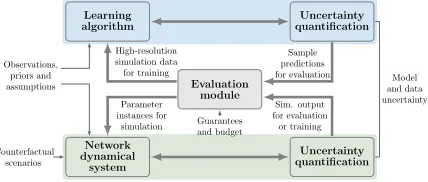
Approach. A schematic of the hybrid system is shown in Figure 1. There are three modules: The
machine learning algorithm, the network dynamical system and evaluation module, which compares the predictions and of both models and directs the exploration of the parameter space until the quality constraints are satisfied. Initially, the network dynamical system is initialized based on assumptions and understanding of agent properties, network structure, etc. Then, it is calibrated using real-world observations of the phenomenon. The learning algorithm can be initially trained using real-world observations, or these observations can be provided along with simulation data at a later stage. After the initialization, an iterative process of interactions between these two models via the evaluation module ensues. The parameters for the evaluation module are the guarantees for prediction and budget constraints such as the maximum number of times the simulator can be invoked. An essential aspect of the framework is to embed uncertainty quantification for both the learning module [33, 34] as well as the dynamical system [35, 36] into the framework.
Evaluation module
Guarantees and budget
Learning
algorithm quantificationUncertainty
Network dynamical system Uncertainty quantification Sample predictions for evaluation High-resolution simulation data for training Parameter instances for simulation Sim. output for evaluation or training Counterfactual scenarios Observations, priors and
assumptions and dataModel
[image:6.612.200.414.362.453.2]uncertainty
Figure 1: Schematic of the hybrid system of machine learning and agent-based simulation system.
The following are some of the key advantages of using such a hybrid framework as opposed to using only its individual components:
Consistency. The network dynamical system can be used to guide the learning algorithm so that
it conforms to the principles and accepted understanding of the phenomenon. At the same time, the learning algorithm will facilitate model selection in a principled manner.
Generalizability. A learning algorithms performance can only be as good as the data provided
to it. Here, we will consider ways in which synthetic data goes beyond the observational data and helps voiding overfitting. We consider two directions. Firstly, we consider dynamical systems whose outputs are at a finer resolution than observation data [37]. Secondly, we will simulate counter-factual scenarios for which no observation data is available. Both aspects are covered in the example.
Efficiency. In applications such as epidemic spread, population networks tend to be large, the
space exploration and calibration is a major challenge. Recently, machine learning surrogates have been considered to efficiently explore the parameter space and use them to approximate outcomes of the target dynamical system [38]. Some learning algorithms naturally facilitate sensitivity analysis. Algorithms such as decision trees can potentially explain the behavior of the system as well. Much of the work in this regard has been empirical.
2.3 An Illustrative application: Simulation Guided Machine Learning for Epi-demic Forecasting
Data sparsity is often a challenge for applying machine learning, especially deep learning methods to forecasting problems in socio-technical systems. One example of such problems is to predict weekly incidence in future weeks as well as onset and peak of the season in an influenza epidemic. An infectious disease, such as influenza, spreads in a population through a social network via person to person interactions.
In such socio-technical systems, it is costly to collect data by surveillance or survey, and it is difficult or impossible to generate data by controlled experiments. Usually we have only limited observational data, e.g. weekly incidence number reported to the Centers for Disease Control and Prevention (CDC). Such data is of low spatial temporal resolution (weekly at state level), not real time (at least one week delay), incomplete (reported cases are only a small fraction of actual ones), and noisy (adjusted by CDC several times after being published).
The complexity of the dynamics in such a large scale social network, due to individual level heterogeneity and behavior, as well as interactions among individuals, makes it difficult to train a machine learning model that can be generalized to patterns not yet presented in historical data. Completely data driven models cannot discover higher resolution details (e.g. county level inci-dence) from lower resolution ground truth data (e.g. state level inciinci-dence).
Statistical methods for epidemic forecasting include generalized linear models (GLM), au-toregressive integrated moving average (ARIMA), and generalized auau-toregressive moving average (GARMA) [39, 40, 41]. [42] proposed a dynamic Poisson autoregressive model with exogenous in-put variables (DPARX) for flu forecasting. [43] proposed ARGO, an autoregressive-based influenza tracking model for nowcasting that incorporated CDC ILINet data and Google search data.
Deep learning methods based on artificial neural networks (ANN) have recently been applied to epidemic forecasting due to their capability to model non-linear processes. Recurrent Neural Network (RNN) has been demonstrated to be able to capture dynamic temporal behavior of a time sequence. [44] built an LSTM model for short-term ILI forecasting using CDC ILI and twitter data. [45] proposed LSTM based method that integrates the impacts of climatic factors and geographical proximity to achieve better forecasting performance. [46] constructed a deep learning structure combining RNN and convolutional neural network to fuse information from different sources.
Both statistical and deep learning methods cannot model heterogeneity at disaggregate levels based on aggregate data, so they have difficulty producing forecasts of a higher resolution than that of observed data. In addition, deep neural networks need large amount of training data. Thus overfitting often happens due to availability of only small amount of historical surveillance data.
models allow them to handle new patterns in data; and depending on the model resolution fore-casts can be made of various resolutions, even down to individual level in case of a detailed agent based model. The major challenge with these causal methods is the high dimensionality of model parameters. Again, sparse ground truth data is not enough to calibrate many parameters. Further-more, the agent based epidemiological models are highly compute intensive, making it non-trivial to search through the parameter space. These models usually demand high performance algorithms to simulate.
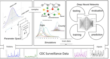
[image:8.612.193.423.383.506.2]To address the challenges posed by data sparsity, we adopt the SimulationTrainedML approach. The idea is to use theory to guide machine learning / deep learning model training. Specifically for epidemic forecasting problem, we take an existing epidemiological model, derive a reasonable distribution of parameter values, sample many configurations of the model from the distribution and run HPC based simulations, then use the synthetic data produced by simulations to train a deep neural network, which can be used for forecasting. This approach integrates epidemiology theory, HPC simulations, and deep learning models under the paradigm of Theory Guided Machine Learning (TGML). It improves generalizability of machine learning models, ensures their physical consistency with the epidemiological models, and enables high resolution forecasting. Simulations can generate required synthetic training data for neural network models with minimal costs (mainly HPC costs). The mechanistic model can not only generate data similar to the observed but also produce data that has never occurred in reality, and allows the trained neural networks to model new patterns. The TGML approach can also easily make long term forecasting of epidemic dynamics using simulations. Furthermore, the behavior modeling in agent based models allows counter-factual analysis and what-if forecasts.
Figure 2: Simulation trained ML
For infectious disease forecasting, we propose DEFSI (Deep Learning Based Epidemic Fore-casting with Synthetic Information), a framework that integrates the strengths of artificial neural networks and causal models. It consists of three components. (1) Disease model parameter space construction: Given an existing agent based epidemic model, we estimate a marginal distribution for each model parameter based on coarse surveillance data. (2) Synthetic training data genera-tion: We generate a synthetic training dataset at high-resolution scale by running HPC simulations parameterized from the parameter space. (3) Deep neural network training and forecasting: We train a two-branch deep neural network model on the synthetic training dataset and use coarse surveillance data as inputs to make detailed forecasts.
Why should we build a reduced order model. A natural question is the need for such
neural network model is developed real-time forecasting is possible. Second, such a model can also be used when one uses simulations for planning and optimization problems and needs forecasted values during the decision making phase. (Needs a bit more cleaning up)
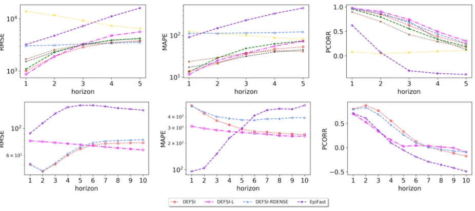
[image:9.612.77.540.218.424.2]We run experiments to evaluate DEFSI against several state-of-the-art epidemic forecasting methods. (1) LSTM (single-layer LSTM) [52]; (2) AdapLSTM (CDC + Weather data) [45]; (3) ARIMA (classic ARIMA) [40]; (4) ARGO (CDC + Google data) [43]; and (5) EpiFast (causal forecasting method based on EpiFast simulations) [49]. The last method can make county level forecasts while the others can only make state level forecasts. Experimental results show that DEFSI performs comparably or better than the other methods for state level forecasting. For county level forecasting, the DEFSI method significantly outperforms the EpiFast method.
Figure 3: Virginia state level forecasting, 2017-2018 (top) and New Jersey county level forecasting, 2017-2018 (bottom).
3
Machine Learning for Virtual Tissue and Cellular Simulations
3.1 Virtual Tissue Models
(105−107), so calculating the temporal changes of cell shape, position and internal state is time consuming. 2) Agents are often hierarchical, with agents composed of multiple agents at smaller scales, and are highly diverse in type. As a result VT simulations must explicitly represent a very broad range of length and time scales (nanometers to meters and milliseconds to years). 3) Agents within and between scales interact strongly with each other, often over significant ranges [57]. Ex-plicit models of long range force transduction and reorganization of the complex fiber networks [60] of extracellular matrix outside of cells and of the active cytoskeletal fiber networks inside of cells are particularly challenging. Solid mechanics models of bulk material deformations are also challenging. 3) Individual agents typically contain complex network sub models which control their properties and behaviors, e.g., of cell regulation, signaling and metabolism. 4) Materials properties may be complex, like the shear thickening or thinning or swelling or contraction of fiber networks, which may be individually expensive to simulate. 5) Modeling transport is also challenging. Agents exist in a complex environment, which governs the transport of multiple chemical species. In many VT simulations, the solution of the diffusion equation (with complex rules for active and passive boundary crossing) for many species under complex, every-changing conditions is the most com-putationally expensive part of the simulation. In other cases, e.g. when there is significant flow of blood or interstitial fluid, or bulk material movement, transport requires the solution of complex advection diffusion equations.6) Models are typically stochastic, so predictivity requires execution of many replicas under identical conditions. Importantly, this stochasticity usually does not rep-resent error–different simulation outputs for the same parameters are both valid and the average of two valid solutions is not generally a valid solution. E.g., a vascular growth experiment which can generate two different random spatial vascular structures, or where two qualitatively different results where the interest is the probability of occurrence of an outcome–e.g. Does a cancer metas-tasize or not and if so, to what organ? 7) Simulations involve uncertainty both in model parameters (there may be hundreds of parameters, many of them poorly quantified) [61] and in model structure (the actual set of interaction rules and types). The former means that parameter optimization and uncertainty quantification are hard, the latter is worse, because the combinatorics involve searches over complex response surface spaces in which gradient methods dont work. 8) Biological and medical time-series data for concentrations or states are often qualitative, semiquantitative or dif-ferential, making their use in classical optimization difficult (their use requires the definition of case-specific metrics and their weighted inclusion in the definition of residuals–outcomes are often sensitive to this weighting and we lack formal ways to optimize these weights). 9) In many cases, time series for validation may not be synchronized with model time points (in terms of starting time, ending time or time rates). 10) VT models often produce movies of configurations in 2D x time or 3D x time. In general, we lack appropriate general metrics to compare experimental movies to VT outputs (and we have the additional issue of scaling, region of interest limitation and regis-tration, as well as stochasticity), making feature-extraction and classical optimization problematic. 11) Finally, given the complexity of VT models and their simulation, there is the additional com-putational challenge of simulating populations of individuals. Simulation of a population can add several additional orders of magnitude to the computational challenge. Unsupervised learning, can, in principle, handle stochasticity, determine appropriate weights, registration and features to allow comparison between experiment and simulation.
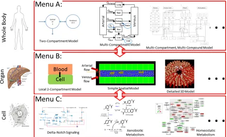
Figure 4: Multiscale VT simulations often include sub-models for particulate scales. For example, the whole body is represented as a PBPK model, coupled to a VT model, with each agent (e.g., cell) in the VT model coupled to a subcellular model. This approach typically, and optimally, uses different modeling modalities at each scale. Constructing a model in this manner allows simulations to include experimental data obtained from different sources. For example, the PBPK scale is suitable for including systemic measurables such as blood concentration versus time following a dose of a xenobiotic. The subcellular scale can often be calibrated using measurements from cell culture assays. There are often multiple possible models at a particular scale that differ in their level of detail.
the possibility of varying levels of details greatly increases the level of complexity. It is possible that ML techniques can be used to short circuit implementations at individual scales.
Perhaps surprisingly, given the above caveats, virtual tissue models can and do generate sci-entifically and practically meaningful results in a wide variety of cases, and some are even used clinically on a regular basis for the optimization of personalized therapies.
Secondly, a growing number of general modeling frameworks, CompuCell3D, PhysiCell [62], Morpheus, Neuron, VirtualCell, allow the high-level specification of VT simulations of different types. These frameworks typically share an approach to modularization, built around the definition of object classes and their properties, behaviors and interactions. Models are increasingly structured as pluggable components, which can be refined by inclusion of more detailed submodels or replaced by coarse-grained approximations.
3.2 Virtual Tissue Modelling and AI
1. Short-circuiting: The replacement of computationally costly modules with learned analogues. E.g. in the case of diffusive transport, we want to know the flux of a given chemical species at a given location given the global pattern of sources and sinks of the species, without having to solve the diffusion equations. In the case of a model of the heart we want to know the stress distribution in the heart tissue from the unstressed geometry of the heart and its current geometry, without having to solve the nonlinear solids equations which relate stress and strain in this complex material. In both cases, there are proof-of-principle demonstrations that such short-circuiting is possible and can speed up calculations by many orders of magnitude.
2. Parameter optimization in very high dimensional parameter spaces. VT models are typically significantly overfitted (not enough validation data for the hundreds of parameters), but the sets of parameters which lead to equally good solutions are of interest.
3. Model reduction and uncertainty quantification–the analysis of conditions under which pa-rameters or model elements are unnecessary and can be eliminated from the simulation.
4. Encapsulation (coarse graining)–Can you take a bunch of agents, put a box around them and simulate the input-output relations of the box? A classic example of this is the diffi-culty of deriving meaningful bulk materials parameters from the microstructure of ECM or cytoskeletal components. The key challenge is the lack of homogeneity in biological systems that means that classical approaches to coarse-graining fail.
5. Approaches to treating stochasticity of results as information rather than noise.
6. In many cases the exact quantitative values of the simulation prediction are critical (the contraction efficiency of the heart, a surgical the safety margin around an MRI image of a tumor) and we would be using AI to interpolate between directly simulated results. In other cases, we are primarily interested in the bifurcation structure of the model with respect to one or more parameters (as a concentration of a chemical increases, a circuit goes from stable to oscillatory behavior). In the latter case we want to use AI approaches to predict the range of possible output configurations from input structures (classification) to address problems where model structure is uncertain.
7. The design of maximally discriminatory experiments for hypothesis testing is a key application of VT models–the use of AI to predict the (experimentally realizable) parameter sets for which two models with different hypotheses have the most distinct results would greatly facilitate the application of modeling to experiment.
8. A particular area of interest is the use of AI to run time backwards, to allow the design of initial conditions which lead to desired outputs–such inverse time simulation is especially critical to enable tissue engineering applications of VTs.
9. Another area of interest is the elimination of short time scales–in particular, the rate of blood flow is very fast compared to other tissue-level time scales. If AI can short-circuit the calculations of advection-diffusion transport, it would speed up typical tissue calculations by several orders of magnitude.
determine if a VT simulation has generated a tissue which structurally resembles its exper-imental counterparts. Currently, such classification is not possible using predefined feature extractions methods.
In each of these cases, a VT model has the advantage that it can generate limitless amounts of training data (albeit at high computational cost).
3.3 Multiscale Biological Modelling and MLandHPC
Therefore, there are several areas in multiscale biological modeling that could benefit from advances in MLforHPC. Such as;
1. Generation of additional multiscale time series from limited experimental data (detailed time series data is expensive to obtain). The ability to extract fundamental characteristics of the system, without necessarily developing deep mechanistic understanding of the controlling equations or parameters. Create ”synthetic, complex time series data” that is consistent with the limited amount of experimental data.
2. Generation of multiscale time series across species. Leverage much larger data sets in ex-perimental animals to extend the limited data in humans. E.g., map animal to human data including stochasticity and inter-individual variation.
3. Extraction of commonalities across VT simulations. For example, multiple VT models, each for a particular disease, share a common PBPK backbone. Use AI to extract parameters (and parameter ranges) that are VT-model independent such as apparent tissue volumes, blood flow rates etc.
4. Use of AI to score the ”biological possibility” of a computationally constructed representation (e.g., a replicates) of a biological system. In particular for 2D and 3D tissue models used as replicates in VT simulations. If an AI classifier can differentiate between real 2D/3D data and synthetic data, then the synthetic data does not adequately represent reality.
5. Prediction of crashes in simulations. When exploring large parameter spaces it is often the case that certain sets of parameters result in either a numerical crash of the simulation or the simulation straying into a non-biologically possible region. MLfor HPC techniques that can monitor a large scale simulation project and develop predictors for when particular parameter sets may give invalid results allowing those simulations to be skipped.
Key concerns about AI replacement of model components include: 1) The accuracy of learned interpolations within the span of the training set, 2) the range of parameters outside of the training set span over which model prediction is qualitatively correct. 3) The efficiency of learning over very sparse training sets. 4) The ability to train when the same input data can lead to very different output data sets (in other words, where the inputs lead not to a single deterministic output, but to a complex range of outputs each of which is valid in its own right). Thus, classical back propagation algorithms may need to be rethought to handle the multivalency of outputs. 5) Model structure inference is challenging, because there is not necessarily a differentiable way to transition between models with different structures for gradient methods (unless we use systems with very high combinatorial complexity–all-to-all couplings).
robust to stochasticity and drift of parameters (e.g., changing the concentration of a key input chemical by a factor of ten has no measurable effect on system outputs), but failures tend to be dramatic (e.g. the transition between a regulated stem cell state and a cancer). This robustness makes the predictability of normal situations more credible, but also that divergences between AI predictions and reality may be abrupt and dramatic rather than gradual.
Prior work by Karniadakis [22, 63], Kevrekidis [21] and Nemenman [64] have shown that neural networks can effectively learn to reproduce the temporal behaviors of fairly complex biochemical regulatory and signaling networks over a broad range of physiological conditions. This ios comple-mented by successful applications in other domains [65]. Liang-liang [66] has shown that networks can also learn to short-circuit nonlinear biomechanics simulations of the aorta–being able to predict the stress and strain distribution in the human aorta from the morphology observable with MRI or CT alone. These successes provide important proof-of-principle for the use of AI to enhance VT simulations. However, the typical VT model is much more complex than these biological models. VTs typically involve the change of position and state of hundreds of thousands or millions of agents, each of which has complex internal control and complex deformable shape. In this sense, the use of AI is more similar to the use of AI to play a very extended version of the game of Go than to learn the behavior of a classical dynamical system. E.g. the dimensionality of the inputs for the spatial components of a VT is very high (the 3D positions, shape and surface and volume proper-ties of every agent in the simulation). Many of these issues represent significant computer-science research problems.
We plan the investigate 3 separate projects which will demonstrate the utility of AI methods in accelerating and improving VT simulations.
1. Project 1: Focus–Parameter and model structure estimation in challenging conditions. Test
the ability of various back-propagation methods to infer VT model parameters from stochastic simulation outputs for different levels of model complexity. Study the degradation of predic-tion as the number of parameters increases and the number of simulapredic-tion replicas decreases to determine a heuristic trade-off for model inferability. Test the ability of AI to identify possible regulatory circuits for control of known biological systems.
2. Project 2: Focus–Short-circuiting of high dimensional models for acceleration. Develop a
short-circuit diffusion solver which takes spatial source, sink and boundary geometries and conditions and returns the chemical concentration at a desired location and net fluxes over all boundary surfaces. Apply this accelerator to a VT model of a vascular tumor. Study the numerical accuracy of the field predictions and the range of situations in which the AI approximation becomes qualitatively wrong rather than numerically inaccurate. If the base diffusion solver works, extend to include a model of vascular transport via a capillary network.
3. Project 3–Focus–Coarse graining. Train a network on a microscopic model of fiber dynamics
and reaction-advection-diffusion interactions and their effect on cell movement and polariza-tion under representative condipolariza-tions. Attempt to predict the dynamics of cell polarizapolariza-tion (both mesenchymal to epithelial transition and lamellipodial polarization of fibroblasts) from internal state and external conditions.
4
Machine Learning for Molecular and Nanoscale Simulations
4.1 MLaroundHPC for nanoscale simulation
4.1.1 Example
We start with a simple example to provide context and illustrate the value of MLaroundHPC in the nanoscale simulation domain. Consider a typical coarse-grained (with implicit solvent) molecular dynamics (MD) simulation of ions confined at the nanoscale: 1 nanosecond of dynamics (1 million computational steps) of a system of 500 ions on one processor takes about 12 hours of runtime, which is prohibitively large to extract converged results within reasonable time frame. Performing the same simulation on a single node with multiple cores using OpenMP shared memory accelerates the runtime by a factor of 10 (≈1 hour), enabling simulations of the same system for longer physical times leading to more accurate results within reasonable computing time. The use MPI can dra-matically enhance the performance of these simulations: for systems of thousands of ions, speedup of over 100 can be achieved, enabling the generation of accurate data for evaluating ionic distri-butions. Further, a hybrid OpenMP/MPI approach can provide even higher speedup of over 400 for similar-size systems enabling state-of-the-art research on the ionic structure in confinement via simulations that explore the dynamics of ions with less controlled approximations, accurate poten-tials, and for tens or hundreds of nanoseconds over a wider range of physical parameters. However, despite the employment of the optimal parallelization model suited for the size and complexity of the system, scientific simulations remain time consuming. In research settings, simulations can take up to several days and it is often desirable to foresee expected overall trends in key quantities; for example, how does the contact density vary as a function of ion concentration in the confinement. Long-time simulations and investigations for larger system sizes become prohibitively expensive. The situation gets increasingly worse as the models become more fine-grained. Explicit solvent leads to a dramatic decrease in computational performance. The above example is illustrative of the general problem in simulation of materials at the nanoscale; self-assembly phenomena associated with capsomeres assembling into a viral capsid or with assembly of functionalized nanoparticles into higher-order structures exhibit similar computational challenges.
4.1.2 Why MLaroundHPC and what does it enable
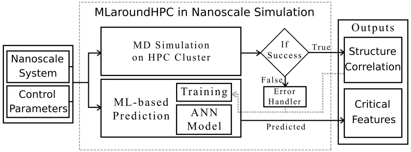
Given the powerful rise in ML and HPC technologies, it is not the question of if, but when, ML can be integrated with HPC to advance simulation methods and frameworks. It is critical to understand and develop the software frameworks to build ML layers around HPC to 1) enhance simulation performance 2) enable real-time and anytime engagement, and 3) broaden the appli-cability of simulations for both research and education (in-classroom) usage. Some early work in using ML in material simulations and scientific software applications (see Sec. 4.1.3) has already begun in this direction further inspiring the research objectives. Figure 5 shows a schematic of the MLaroundHPC framework for a generic nanoscale simulation. The goal is typically to predict the structure or correlation functions (outputs) characterizing the nanoscale system over a broad range of experimental control parameters (inputs). As Figure 5 shows, MLaroundHPC can enable the following outcomes:
1. Learn pre-identified critical features associated with the simulation output (e.g. key experimentally-relevant quantities such as contact ionic density in the above example or nanoparticle pair correlation functions in nanoparticle self-assembly simulations).
3. Exhibit auto-tunability (with new simulation runs, the ML layer gets better at making pre-dictions etc.)
4. Enable real-time, anytime, and anywhere access to simulation results from trained ML models. (particularly important for education use).
5. No run is wasted. Training needs both successful and unsuccessful runs.
MLaroundHPC in Nanoscale Simulation
Critical Features Structure Correlation Nanoscale
System
[image:16.612.95.514.182.337.2]Control Parameters
Figure 5: Schematic of the MLaroundHPC framework in nanoscale simulation.
To further illustrate these goals, we discuss an application related to the example simulation presented above in Sec. 4.1.1. The distribution of electrolyte ions near charged or neutral nano-materials such as nanoparticles, colloids, or biological macromolecules determines their assembly behavior. As a result, the computation of structure of ions confined by surfaces that are nanome-ters apart has been the focus of several recent experiments and computational studies [67, 68, 69]. Simulations of such coarse-grained models have been employed by many researchers to extract the ionic distributions confined between the interfaces for a wide range of parameters such as elec-trolyte concentrations, ion valencies, and interfacial separations [70, 71, 68]. Simulations have been performed using customized codes developed in individual research groups [70, 72, 68] or general purpose software packages such as ESPRESSO [73] and LAMMPS [74].
artificial neural network successfully learned the desired features associated with the output ionic density profiles and rapidly generated predictions that are in excellent agreement with the results from explicit molecular dynamics simulations.
4.1.3 Related work
Traditionally, performance enhancement of scientific applications has largely been based on improv-ing the runtime of the simulations usimprov-ing parallel computimprov-ing methods, includimprov-ing different acceleration strategies such as OpenMP, MPI, and hybrid programming models. Recent years have seen a surge in the use of ML to accelerate computational techniques aimed at understanding material phe-nomena. ML has been used to predict parameters, generate configurations in material simulations, and classify material properties [78, 79, 80, 81, 82, 83, 84, 85, 86, 87]. For example, Fu et al. [81] employed ANN to select efficient updates for Monte Carlo simulations of classical Ising spin models that overcome the critical slowing down issues in Monte Carlo simulations. Similarly, Botu et al. [84] employed kernel ridge regression (KRR) to accelerate MD method for nuclei-electron systems by learning the selection of probable configurations in MD simulations, which enabled bypassing explicit simulations for several steps.
4.2 MLaroundHPC for biomolecular simulations
4.2.1 Current work
The use of ML and in particular DL approaches for biomolecular simulations is still in its infancy compared to other areas such as nano-science and materials science. This might be partly due to the large system sizes (100,000 of atoms), the importance of solvent (water, ions, lipids for membrane proteins), the high level of heterogeneity, and possibly the importance of both short range ( 10 ) and long range (electrostatic) interactions. Current work in this area originated in materials sciences [88, 89]. One promising approach is based on work by Behler and Parrinello [90] who devised a very efficient and accurate NN-based potential that was trained on quantum mechanical DFT energies; their key insight was to represent the total energy as a sum of atomic contributions and represent the chemical environment around each atom by an identically structured NN, which takes as input appropriate symmetry functions that are rotation and translation invariant as well as invariant to exchange of atoms but correctly reflect the local environment that determines the energy [88]. Based on this work, Gasteggeret al. [91] used ML to accelerate ab-initio MD (AIMD) to compute accurate IR spectra for organic molecules including the biological Ala+3 tripeptide in the gas phase. They employed Behler-Parrinello HDNNP (high-dimensional neural network potentials) and an automated sampling scheme to converge HDNNPs but they did not perform on-the-fly training due to the high cost of DFT energy evaluations. Interestingly, the ML model was able to reproduce anharmonicities and incorporate proton transfer reactions between different Ala+3 tautomers without having been explicit trained on such a chemical event, highlighting the promise of such an approach to incorporate a wide range of physically relevant effects with the right training data. The ML model was>1000 faster than the traditional evaluation of the underlying quantum mechanical physical equations.
energy calculations without tight coupling between the training and the simulation steps. Exten-sions of their work (improving NN generation with an active learning (AL) approach via Query by Committee (QBC)) demonstrated that proteins in an explicit water environment can be simulated with a NN potential at DFT accuracy [93]. The AL approach reduced the amount of required training data to 10% of the original model [93] by iteratively adding training data calculations for regions of chemical space where the current ML model could not make good predictions. Us-ing transfer learnUs-ing, the ANI-1 potential was extended to predict energies at the highest level of quantum chemistry calculations (coupled cluster CCSD(T)), with speedups in the billions [94].
4.2.2 Outlook
In general the focus has been on achieving DFT-level accuracy. Speeding up classical MD sim-ulations with empirical force fields has not been attempted, likely because the empirical energy functions are typically simpler than the NN potentials and so the computational cost of evaluating a NN potential is higher than or on par with evaluation of a classical empirical potential. How-ever, replacing solvent-solvent and solvent-solute interactions, which typically make up 80%-90% of the computational effort in a classical all-atom, explicit solvent simulation, with a NN potential promises large performance gains at a fraction of the cost of traditional implicit solvent models and with an accuracy comparable to the explicit simulations, as already discussed above in the case of electrolyte solutions. Furthermore, inclusion of polarization, which is expensive (factor 3-10 in current classical polarizable force fields) but of great interest when studying the interaction of multivalent ions with biomolecules might be easily achievable with appropriately trained ML potentials.
An interesting question is if ML potentials can be used to push the typical time step size in the integration of the classical equations of motions to times beyond the 2–5 fs that are currently feasible. Experience from heuristic coarse grained force fields [95, 96] shows that smoothing of the energy landscape by coarse graining allows much larger time steps, e.g. 10 - 20 fs. If ML potentials can be shown to also coarse-grain the energy landscape in a similar fashion then an enhancement of sampling and speedup of factors of 2–5 might be possible, at effectively the same accuracy as traditional classical all atom MD simulations. This assumes that ML potentials somehow capture dynamics on a low-dimensional manifold on which the energies and forces vary more smoothly than on the full 6N phase space [97].
5
Cyberinfrastructure and Computer Science Background for the
Integration of Machine Learning and HPC
5.1 HPC for Machine Learning
owing to the fact that computation is irregular and the model size can be huge. At the meantime, parallel workers need to synchronize the model continually. By investigating collective vs. asyn-chronous methods of the model synchronization mechanisms, we discover that optimized collective communication can improve the model update speed, thus allowing the model to converge faster. The performance improvement derives not only from accelerated communication but also from re-duced iteration computation time as the model size may change during the model convergence. To foster faster model convergence, we need to design new collective communication abstractions. We identify all 5 classes of data-intensive computation[2], from pleasingly parallel to machine learning and simulations. To re-design a modular software stack with native kernels to effectively utilize scale-up servers for machine learning and data analytics applications. We are investigating how simulations and Big Data can use common programming environments with a runtime based on a rich set of collectives and libraries for a model-centric approach [107, 108].
5.2 Parallel Computing
We know that heterogeneity can lead to difficulty in parallel computing. This is extreme for MLaroundHPC as the ML learnt result can be huge factors (105 in our initial example[77]) faster than simulated answers. Further learning can be dynamic within a job and within different runs of a given job. One can address by load balancing the unlearnt and learnt separately but this can lead to geometric issues as quite likely that ML learning works more efficiently (for more potential simulations) in particular regions of phase space.
5.3 Scaling of Effective Performance
An initial approach to estimate speedup in a hybrid MLaroundHPC situation is given in [77] for a nano simulation. One can estimate the speedup in terms in terms of four timesTseq the sequential execution time of simulation;Ttrain the time for the parallel execution of simulation to give training data; Tlearn is the time per sample to train the learning networkl; andTlookupis the inference time to predict the results of the simulation by using the trained network. In the formula below,Nlookup is the number of trained neural net inferences and Ntrain the number of parallel simulations used in training.
Effective Speedup S = Tseq(Nlookup+Ntrain)
TlookupNlookup+ (Ttrain+Tlearn)Ntrain
This formula reduces to the classic simple Tseq
Ttrain when there is no machine learning and in the limit
of large Nlookup
Ntrain becomes
Tseq
Tlookup which can be huge!
There are many caveats and assumptions here. We are considering a simple case where one runs the Ntrain simulations, followed by the learning and then all the Nlookup inferences. Further we assume the training simulations are useful results and not just overhead. We also have not properly considered how to build in the likelihood that training, learning and lookup phases are probably using different hardware configurations with different node counts.
6
Uncertainty Quantification for Deep Learning
can only learn X-Y NOT X and Y separately. Further, use of reduced precision in DL networks needs to be re-examined for our application.
The bias-variance trade-off is a well-studied concept in statistical learning that can provide a principled way to design a machine learning model concerning its complexity given the optimization problem and the dataset [109]. It is based on the decomposition of the expected error that a model can make into two parts: variance and bias. The variance part explains the uncertainty of a model due to the randomness in the training algorithms (e.g. random initialization of parameters or a different choice of hyperparameters) or the lack of representativeness of the subsampled training set used in training. One can reduce the variance of the expected error by introducing a regularization scheme during the optimization process so that the model complexity is in control and can result in a smoother model. However, the regularization approach comes at the cost of an increased amount bias, which is another term in the expected error decomposition that explains the fitness of the model to the currently available dataset. By reducing the flexibility of the model using a regularization scheme, the training algorithm can only do a limited effort to minimize the training error. On the contrary, an unregularized model with a higher model complexity than necessary can also result in a minimal training error in that training session, while it suffers from high variance or uncertainty in its prediction.
Ideally, the bias-variance trade-off can be resolved to some degree by averaging the trained instances of a complex model. As the variance term explains the statistical deviations of the different model predictions from their expected value, one can reduce it by training many model instances and average out their variations. Once these model instances are complex enough to fit the training dataset, we can use the averaged predictions as the output of the model. However, averaging many different model instances implies a practical difficulty that one has to conduct multiple optimization tasks to come up with a statistically meaningful sample distribution of the predictions. Given the assumption that the model might as well be a complex one to minimize the bias component (e.g. a deep neural network), model averaging is computationally challenging. Also, for a real-world problem that needs as much labeled dataset as possible, subsampling might not be the best way to make use of the data.
Dropout has been extensively used in deep learning as a regularization technique [110, 111, 112, 113], but recent researches revisit it as an uncertainty quantification (UQ) tool as well [114, 33]. The use of dropout as a tool for acquiring the sample distribution of predictions can be justified by the fact that the dropout procedure on a deep neural network (DNN) can be seen as an efficient way to maintain a pool of multiple network instances for the same optimization task. The efficiency of the procedure comes from the fact that the dropout technique applies a Bernoulli mask to the layer-wise feature vector, a stochastic structure alteration process, to each of the feedforward routines under the stochastic gradient descent training framework. Thus, the training process has the same effect as if it is exposed to many network instances although training is on only one instance. Dropout has shown promising performances in many deep learning benchmarks especially thanks to its ability to prevent overfitting. Although the original usage of dropout has been limited to the regularization during training, recent researches suggest its use during the test time as well. As the network trained with the dropout technique is robust to the structural variation, during the test time one can use the same masking strategy to come up with a set of differently thinned versions of the network, which can form a sample distribution of predictions. Hence, the access to the distribution of the predictions enables one to use it as a UQ metric of the trained deep learning system.
more data in large-scale machine learning tasks causes a lack of data, as the ML applications that try to catch up human perception in classification tasks, e.g. visual object recognition, require the data examples to be labeled by humans. Crowdsourcing can reduce the cost of generating such a labeled dataset [115]. However, as for modeling the large-scale simulation results, the ML model has to see more examples generated from the HPC simulation, which is a conflicting requirement as the purpose of training ML is to avoid such computation. The UQ scheme can play a role here to provide the training routine with a way to quantify the uncertainty in the prediction—once it is low enough, the training routine might less likely need more data.
7
Machine Learning Requirements for MLforHPC
Here we review the nature of the Machine Learning needed for MLforHPC in different application domains. The Machine Learning (ML) load depends on 1) Time interval between its invocations, which will translate into the number of training samples S and 2) size D of data set specifying each sample. This size could be as large as the number of degrees of freedom in simulation or could be (much) smaller if just a few parameters are needed to define simulation. We note two general issues
• There can very important data transfer and storage issues in linking the Simulations and Machine Learning parts of system. This could need carefully designed architectures for both hardware and software.
• The Simulations and Machine Learning subsystems are likely to require different node opti-mizations as in different types and uses of accelerators.
7.1 Nanosimulations
In each of two cases below, one is using scikit-learn, Tensorflow and the Keras wrapper for Tensor-flow, as the ML subsystem. The papers [77, 116] are using ML to learn results (ionic density at a given location) of a complete simulation
• D=5 with the five specifying features as connement length h, positive valency zp, negative valencyzn, salt concentration c, and the diameter of the ions d.
• S= 4805 which 70% of total 6864 runs with 30% of the total runs used for testing.
In [23], one is not asking ML to predict a result as in [77],but rather training an Artificial Neural Net (ANN) to ensure that the simulation runs at its optimal speed (using for example, the lowest allowable timestep dt and ”good” simulation control parameters for high efficiency) while retaining the accuracy of the final result (e.g. density profile of ions). For this particular application, we could get away by dividing a 10 million time-step run ( 10 nanoseconds that is a typical timescale to reach equilibrium and get data in such systems) into 10 separate runs.
• Input data size D= 6 (1 input uses 64 bits floats and 5 inputs use 32 bits integers - total 224 bits)
• Input number of samples (S) = 15640 (70% training 30% test) • Hidden layer 1 = 30
• Hidden layer 1 = 48 • Output variables = 3
million steps long, and you use/learn/train ML every 1 million steps (so block size is a million), yielding 10 times more samples than runs.
Generalizing this, the hardware needs will depend on how often you block, to stop and train the network, and then either on-the-fly or post-simulation, use that training to accelerate simulation or evaluate structure respectively. Blocking every timestep will not improve the training as typically, it won’t produce a statistically independent data point to evaluate any structure you desire. So you want to block at a timescale that is at least greater than the autocorrelation time dc; this is, of course, dependent on example you are looking at – and so your blocking and learning will depend on the application. In [77], it is small and dc is 3-5 dt; in glasses, it can be huge as the viscosity is high; and in biomolecular simulations, it will also depend on the level of coarse-graining and will be different in fully atomistic or very coarse-grained systems.
The training effort will also depend on the input data size D, and the complexity of the rela-tionship you are trying to learn which change the number of hidden layers and nodes per layer. For example, suppose you are tracking a particle (a side atom on a molecule in a typical nanoscale simulation), in order to come up with a metric (e.g. distance between two side atoms on different molecules) to track the diversity of clusters of particles during the self-assembly process. This comes from expectation that correlations between side atoms may be critical to a macroscopic property (such as formation of these particles into a FCC crystal). In this case your D is huge, and your ML objectives may be looking for a deep relationship, and you may have to invoke an ensemble of ANN’s and this will change hardware needs.
8
New Opportunities and Research Issues
8.1 Broken Abstractions, New Abstractions:
In traditional HPC the prevailing orthodoxy is Faster is Better which has driven the quest for abstractions of hierarchical parallelism to speeding up single units of works. However the new paradigm in HPC — Learning Everywhere, implies new performance, scaling and execution ap-proaches. In this new paradigm, multiple, concurrent heterogeneous units of work replace single large units of works, which thus require both hierarchical (vertical) parallelism as well horizontal parallelism Relinquishing the orthodoxy based upon hierarchical (vertical) parallelism as the only route to performance is necessary while supporting the scaling requirements of ”Learning Every-where”. Our distinction between traditional performance and the effective performance achieved by using learnt results is important here.
8.2 Research Issues in MLforHPC
Research issues reflect the multiple interdisciplinary activities linked in our study of MLforHPC.
• MLforHPC Cyberinfrastructure • ML and Deep Learning
• Uncertainty Quantification
• Multiple application domains described in sections 2, 3, 4.1 and 4.2
• Coarse graining studied in our case for network science and nano-bio areas
We have identified the following research areas.
2. Which ML and DL approaches are most relevant and how can they be set up to enable broad user-friendly MLaroundHPC and MLautotuning in domain science
3. How can Uncertainty Quantification be enabled and separately study ergodicity (bias) and accuracy issues?
4. Is there new area of algorithmic research focusing on finding algorithms that can be most effectively learnt?
5. Is there a general multiscale approach using MLaroundHPC.
6. What are appropriate systems frameworks for MLaroundHPC and MLautotuning. For exam-ple, should we wrap microservices invoked by a Function as a Service environment? Where and how should we enable learning systems? Is Dataflow useful?
7. The different characters of surrogate and real executions produce system challenges as surro-gate execution is much faster and invokes distinct software and hardware. This heterogeneity gives challenges for parallel computing, workload management and resource scheduling (het-erogeneous and dynamic workflows). The implication for performance is briefly discussed in sections 5.2 and 5.3.
8. Scaling applications that are composed of multiple heterogeneous computational (execution) units, and have distinct forms of parallelism that need balanced performance. Consider a workload comprised of NL learning units, NS simulations units. The relative number of learning units to simulation units will vary with application and problem type. The relative values will even vary over execution time of the application, as the amount of data generated as a ratio of training data will vary. This requires runtime systems that are capable of real-time performance tuning and adaptive execution for workloads comprised of multiple heterogeneous tasks.
9. The application of these ideas to statistical physics problems may need different techniques than those used in deterministic time evolutions.
10. The existing UQ frameworks based on the dropout technique can provide the level of certainty as a probabilistic distribution in the prediction space. However, it does not always mean that the quality of the distribution is dependent on the quality/quantity of data. For example, two models with different dropout rates can produce different UQ results. If the goal of UQ in MLaroundHPC context is to supply only an adequate amount of data, we need a more reliable UQ method tailored for this purpose rather than the dropout technique that tends to manipulate the architecture of the model.
11. Application agnostic description and defintion of effective performance enhancement.
12. Sean Blanchard [117] has emphasized the potential value of learnt information in fault toler-ance where for example learnt results could be used to restart a crashed compute node.
8.3 Possible Dataflow MLforHPC System Architecture
We have advocated in [118] a prototype system approach to MLforHPC that is based on the dataflow representation of the simulation or ML problem where the idea is to support ML wrapping of any dataflow node. This dataflow representation is seen in Big Data systems such as Storm, Heron, Spark, and Flink. We will allow coarse-grain dataflow with dataflow nodes at the job level; this is familiar from workflow systems such as Kepler, Pegasus, and NiFi and illustrated by Persona’s [119] integration of Tensorflow into bioinformatics pipelines. We will also allow finer grain size dataflow as seen in modern big data systems and Function as a Service architectures and provide a cleaner architecture with a single approach to ML integration at all granularity’s. In this discussion, dataflow can be also be considered as a task graph. The chemistry potential example shows a case where the surrogate replaces a fine grain node. The Indiana University Twister2 system [120, 121, 122] supports such a hybrid coarse/fine grain dataflow graph specifying a problem. We intend the same architecture to support both MLaroundHPC and MLautotuning. As emphasized by Sharma [123], one should explore a range of synchronization and data consistency techniques [124] that have been proposed for distributed ML training. These techniques differ from BSP and strong-consistency, and offer a more relaxed consistency model by exploiting and tolerating staleness. We can explore the appropriate consistency model for integrating ML with conventional HPC applications. Examples have been shown [125, 126, 127] of the successful use of relaxed consistency for certain HPC applications including our Harp project [107, 108] where the trade-off of the staleness of the model versus synchronization cost was explored.
Acknowledgments
This work was partially supported by NSF CIF21 DIBBS 1443054 and nanoBIO 1720625; the Indiana University Precision Health initiative and Intel through the Parallel Computing Center at Indiana University. JPS and JAG were partially supported by NSF 1720625, NIH U01 GM111243 and NIH GM122424. SJ was partially supported by ExaLearn – a DOE Exascale Computing project.
References
[1] Geoffrey Fox, James A. Glazier, JCS Kadupitiya, Vikram Jadhao, Minje Kim, Judy Qiu, James P. Sluka, Endre Somogyi, Madhav Marathe, Abhijin Adiga, Jiangzhuo Chen, Oliver Beckstein, and Shantenu Jha. Learning Everywhere: Pervasive machine learn-ing for effective High-Performance computation. Technical report, Indiana University, February 2019. https://arxiv.org/abs/1902.10810,http://dsc.soic.indiana.edu/ publications/Learning_Everywhere_Summary.pdf.
[2] Geoffrey Fox, Judy Qiu, Shantenu Jha, Saliya Ekanayake, and Supun Kamburugamuve. Big data, simulations and HPC convergence. In Springer Lecture Notes in Computer Science LNCS 10044, 2016.
[3] Dennard scaling. https://en.wikipedia.org/wiki/Dennard\_scaling.