2011
Fully Analytic Energy Gradient in the Fragment
Molecular Orbital Method
Takeshi Nagata
National Institute of Advanced Industrial Science and Technology
Kurt Ryan Brorsen
Iowa State University
Dmitri G. Fedorov
National Institute of Advanced Industrial Science and Technology
Kazuo Kitaura
National Institute of Advanced Industrial Science and Technology
Mark S. Gordon
Iowa State University, mgordon@iastate.edu
Follow this and additional works at:
http://lib.dr.iastate.edu/ameslab_pubs
Part of the
Chemistry Commons
The complete bibliographic information for this item can be found at
http://lib.dr.iastate.edu/
ameslab_pubs/345
. For information on how to cite this item, please visit
http://lib.dr.iastate.edu/
howtocite.html
.
Fully Analytic Energy Gradient in the Fragment Molecular Orbital
Method
Abstract
The
Z
-vector equations are derived and implemented for solving the response term due to the external
electrostatic potentials, and the corresponding contribution is added to the energy gradients in the framework
of the fragment molecular orbital (FMO) method. To practically solve the equations for large molecules like
proteins, the equations are decoupled by taking advantage of the local nature of fragments in the FMO
method and establishing the self-consistent
Z
-vector method. The resulting gradients are compared with
numerical gradients for the test molecular systems: (H
2O)
64, alanine decamer, hydrated chignolin with the
protein data bank (PDB) ID of 1UAO, and a Trp-cage miniprotein construct (PDB ID: 1L2Y). The
computation time for calculating the response contribution is comparable to or less than that of the FMO
self-consistent charge calculation. It is also shown that the energy gradients for the electrostatic dimer
approximation are fully analytic, which significantly reduces the computational costs. The fully analytic FMO
gradient is parallelized with an efficiency of about 98% on 32 nodes.
Keywords
Polymers, Electrostatics, Chemical bonds, Proteins, Density functional theory
Disciplines
Chemistry
Comments
The following article appeared in
Journal of Chemical Physics
134 (2011): 124115, and may be found at
doi:10.1063/1.3568010.
Rights
Copyright 2011 American Institute of Physics. This article may be downloaded for personal use only. Any
other use requires prior permission of the author and the American Institute of Physics.
Takeshi Nagata, Kurt Brorsen, Dmitri G. Fedorov, Kazuo Kitaura, and Mark S. Gordon
Citation: The Journal of Chemical Physics 134, 124115 (2011); doi: 10.1063/1.3568010
View online: http://dx.doi.org/10.1063/1.3568010
View Table of Contents: http://scitation.aip.org/content/aip/journal/jcp/134/12?ver=pdfcov
Published by the AIP Publishing
Articles you may be interested in
Nonorthogonal orbital based N-body reduced density matrices and their applications to valence bond theory. II. An efficient algorithm for matrix elements and analytical energy gradients in VBSCF method
J. Chem. Phys. 138, 164120 (2013); 10.1063/1.4801632
Unrestricted Hartree-Fock based on the fragment molecular orbital method: Energy and its analytic gradient
J. Chem. Phys. 137, 044110 (2012); 10.1063/1.4737860
Analytic energy gradient for second-order Møller-Plesset perturbation theory based on the fragment molecular orbital method
J. Chem. Phys. 135, 044110 (2011); 10.1063/1.3611020
Molecular applications of analytical gradient approach for the improved virtual orbital-complete active space configuration interaction method
J. Chem. Phys. 132, 034105 (2010); 10.1063/1.3290203
Theoretical study of intramolecular interaction energies during dynamics simulations of oligopeptides by the fragment molecular orbital-Hamiltonian algorithm method
J. Chem. Phys. 122, 094905 (2005); 10.1063/1.1857481
THE JOURNAL OF CHEMICAL PHYSICS134, 124115 (2011)
Fully analytic energy gradient in the fragment molecular orbital method
Takeshi Nagata (),1,a) Kurt Brorsen,2Dmitri G. Fedorov,1
Kazuo Kitaura (),1,3and Mark S. Gordon ()2
1NRI, National Institute of Advanced Industrial Science and Technology (AIST), 1–1-1 Umezono, Tsukuba,
Ibaraki 305–8568, Japan
2Ames Laboratory, US-DOE and Department of Chemistry, Iowa State University, Ames, Iowa 50011, USA
3Graduate School of Pharmaceutical Sciences, Kyoto University, 46–29 Yoshidashimo Adachi, Sakyo-ku,
Kyoto 606–8501, Japan
(Received 11 November 2010; accepted 28 February 2011; published online 29 March 2011)
TheZ-vector equations are derived and implemented for solving the response term due to the exter-nal electrostatic potentials, and the corresponding contribution is added to the energy gradients in the framework of the fragment molecular orbital (FMO) method. To practically solve the equations for large molecules like proteins, the equations are decoupled by taking advantage of the local nature of fragments in the FMO method and establishing the self-consistentZ-vector method. The resulting gradients are compared with numerical gradients for the test molecular systems: (H2O)64, alanine
decamer, hydrated chignolin with the protein data bank (PDB) ID of 1UAO, and a Trp-cage minipro-tein construct (PDB ID: 1L2Y). The computation time for calculating the response contribution is comparable to or less than that of the FMO self-consistent charge calculation. It is also shown that the energy gradients for the electrostatic dimer approximation are fully analytic, which significantly reduces the computational costs. The fully analytic FMO gradient is parallelized with an efficiency of about 98% on 32 nodes.© 2011 American Institute of Physics. [doi:10.1063/1.3568010]
I. INTRODUCTION
Dynamics simulations of large molecules have become very important in the field of computational chemistry.1–7For example, thermodynamic data such as the free energy and en-tropy can be extracted from such simulations. Since chem-ical processes occur at nonzero temperatures, an increasing number of molecular dynamics (MD) simulations have been performed using model potentials based on molecular me-chanics (MM). Another common use of computational sim-ulations is the sampling of potential energy surfaces for local and global minima using for example, Monte Carlo simula-tions. For instance, the structural data of proteins measured by X-ray or nuclear magnetic resonance (NMR) can be refined with the help of a computational simulation and the result-ing structure stored in the protein data bank (PDB). Classical MM schemes can, in principle, be replaced by more accurate methods that consider the electronic structure explicitly.8–13 The benefit of this replacement is that by using first princi-ples methods, more reliable and sophisticated thermodynamic properties, dynamics, and structures can be provided.
The cost of conventional quantum mechanical (QM) electronic structure approaches formally scales at least asNm, where N measures the size of the molecular system and m ranges from 3 for simple methods [e.g., the local density approximation of density functional theory (DFT)] to much higher values for correlated methods. Considerable efforts are invested in developing linear scaling or O(N) methods.14,15
The fragmentation methods have a fairly long history16–22and
now it is an active area of research.13,23–32
a)Author to whom correspondence should be addressed. Electronic mail:
takeshi.nagata@aist.go.jp. Fax: +81 29 851 5426.
One such method is the fragment molecular orbital (FMO) method.33–36 The FMO method enables the calcula-tion of electronic states for large molecules by performing MO calculations in parallel on fragments of a large molecular system using external electrostatic potentials (ESPs). These ESPs describe the electrostatic field due to charge distribu-tions of all of the other fragments. MOs of individual frag-ments are local in nature, because they are expanded in terms of basis functions on the atoms in the fragments, reducing the computation time significantly. Additionally, in order to re-alize linear scaling, approximations have been proposed for the time-consuming ESP calculation in FMO34,37 and other
methods.10The fragment self-consistent procedure employed
in FMO has been used in somewhat different forms in other methods,18,19,9,38,39 while the many-body expansion of the energy is conceptually related to the theory of intermolecu-lar interactions16or the density expansion method.20
Over the past decade, the FMO method has become one of the most extensively developed fragmentation meth-ods for the calculation of accurate chemical properties, such as the total energy, the dipole moment, and the interac-tion energy between fragments in large systems. The FMO method has been interfaced with many QM methods: Sec-ond order Møller–Plesset (MP2) perturbation theory,40,41
coupled-cluster theory,42 DFT,43,44 Hatree-Fock, the
mul-ticonfiguration self-consistent field method,45 configuration
interaction,46,47 time-dependent DFT,48–50 open-shells51 and
nuclear-electronic orbitals.52For these methods, the total
en-ergies are in good agreement with the corresponding con-ventional QM total energies. The FMO method has been ap-plied to a number of large systems.53–66 FMO–MD has been used67–78to study the dynamics of various processes such as
0021-9606/2011/134(12)/124115/13/$30.00 134, 124115-1 © 2011 American Institute of Physics
chemical reactions. However, the FMO–MD method suffers from an accumulation of errors67with the time evolution due to an incomplete analytic FMO energy gradient.
The analytic FMO energy gradient reported by Kitauraet al. in 2001 (Ref.79) was incomplete since the response term due to the ESPs was neglected assuming that it is a small con-tribution for small basis sets. It was subsequently illustrated that when using larger basis sets, such as 6–31G(d),80 the
re-sponse contribution to the gradient is substantial. Evaluating the response contribution requires the solution of the coupled-perturbed Hartree–Fock (CPHF) equations. These equations are time consuming to solve for large molecules, since they depend not on the fragment size but on the size of the entire system.
Since the original report of a partially analytic FMO gradient,79 several improvements regarding previously miss-ing terms in the FMO gradient have been implemented in the GAMESS program package:81,82 (a) The ESP derivative terms including the Mulliken point charge (PTC) approxi-mation (ESP–PTC),80 (b) the derivative of the dimer energy of two distant fragments approximated as the electrostatic interaction energy (the electrostatic dimer approximation, ES-DIM),83and (c) the hybrid orbital projection derivatives.84
The last and most complicated missing response term is the subject of the present paper in which the exact response term for the FMO ESP gradient contribution is introduced, and the fully analytic FMO energy gradient is implemented, with an additional computation time requirement that is com-parable to the first step of the FMO calculation (the self-consistent charge, SCC, iterations). The gradient implementa-tion is also extended to the ES-DIM approximaimplementa-tion but not yet to the ESP–PTC approximation. Consequently, the usefulness of the FMO method is improved by establishing a complete expression of the analytic energy gradient.
Similarly to FMO, the response term arises in other meth-ods where the external charges are not fully self-consistent. For example, in the electronically embedded method85,86
lay-ers are introduced in the system. This is different from frag-ments because layers are mutually inclusive, i.e., lower layers include higher layers, and thus the lowest layer calculation deals with the whole system, whereas the fragment based ap-proach we take uses the locality of fragments. On the other hand in some other fragment methods such as X-Pol87 the
CPHF-related terms do not arise.
II. FULLY ANALYTIC FMO ENERGY GRADIENT
A. Overview of the FMO energy gradient
In the following equations, the FMO energy expression33–36 and the corresponding gradient
equa-tions are briefly summarized. The two-body FMO (FMO2) total energy is represented as
E= N
I EI +
N
I>J
(EI J −EI −EJ)+ N
I>J
Tr(DI JVI J),
(1)
where EX is the internal fragment energy for fragmentX(X =IorIJ, for monomers and dimers, respectively).VI J is the
matrix form of the ESP for dimerIJdue to the electron den-sities and nuclei of the remaining fragments, i.e.,
VμνI J = K=I J
uKμν+vμνK. (2)
The one-electron and two-electron integrals in VI J μν are, respectively,
uKμν= A∈K
μ| −ZA |r−RA|
|ν, (3)
vμνK = λσ∈K
DλσK (μν|λσ), (4)
where DK
λσ is the density matrix element of fragmentKand (μν|λσ) is a two-electron integral in the atomic orbital (AO) basis. IndexAruns over atoms. The dimer density matrix dif-ferenceDI J in Eq.(1)is defined by
DI J =DI J −(DI ⊕DJ). (5)
We note that the SCC process ensures the self-consistency of monomer densities with respect to each other but not monomer and dimer densities. The direct sum in Eq. (5)means blockwise addition of two monomer matrices into the dimer supermatrix.
The internal fragment energies in Eq.(1)may be written in the form:
EX = μν∈X
DμνX hμνX
+1 2
μνλσ∈X
DμνX DλσX −1 2D
X μλDνσX
(μν|λσ)
+
μν∈X
DμνX PμνX +ENRX , (6)
wherehμνX is theX-mer one-electron Hamiltonian and the nu-clear repulsion (NR) energy is
ENRX = B∈X
A(∈X)>B ZAZB
RA B .
(7)
Note that monomer and dimer densities are determined by the MO calculations in the presence of ESPs due to the remaining monomers. For fragmentation across a covalent bond, the hybrid orbital projection (HOP) contribution
occ
i∈X
2i|PˆX|i = μν∈X
DμνX PμνX, (8)
must be considered in Eq.(6). The HOP operator is defined by
ˆ
PX = k∈X
Bk|θkθk|, (9)
where|θkis a hybrid orbital and the universal constantBkis usually set to 106.
124115-3 Fully analytic energy gradient in FMO J. Chem. Phys.134, 124115 (2011)
The differentiation ofEX with respect to nuclear coordi-natealeads to
∂EX
∂a =
μν∈X DμνX ∂h
X μν ∂a +1 2 μνλσ∈X
DμνX DλσX −1 2D
X μλDνσX
∂(μν|λσ) ∂a
+
μν∈X DμνX ∂P
X μν ∂a −2
occ
i,j∈X
Saj i,XFj iX
−4
occ
i∈X vir
r∈X
Ur ia,XVr iX+∂E
NR X
∂a , (10)
where the overlap derivative matrix element is defined by
Si ja,X = μν∈X
CμXi∗∂S X μν ∂a C
X
νj. (11)
The internal fragment Fock matrix element FX
i j is given in terms of MOs:
Fi jX =hi jX+
occ
k∈X
[2(i j|kk)−(i k|j k)]+Pi jX, (12)
where the MO-based projection operator matrix Pi jX is intro-duced for convenience:
Pi jX = μν∈X
CμXi∗PμνXCνXj. (13)
Throughout this study, the Roman (ijkl· · ·) and Greek (μνρσ· · ·) indices denote the molecular orbitals and AOs, re-spectively. For the response term in Eq. (10), the following equation defined in the previous study80is introduced:
Ua,X,Y =4
occ
i∈X vir
r∈X
Ur ia,XVr iY. (14)
The response termsUr ia,X associated with ESPVY r i in the MO basis arise from the expansion of the MO coefficient derivative in terms of the MO coefficients,88 and Eq. (14) sums the Ur ia,X terms multiplied by the Vr iY terms in order to simplify the gradient derivations. There are two types of Ua,X,Y terms: (a)Ua,I,I (i.e.,X=Y) arising from the deriva-tive of the monomer terms, and (b)Ua,X,I J whereXcan beI, J, orIJ[related to the threeDterms in Eq.(5)]. The deriva-tives of the MO coefficients can be written as
∂CX μi
∂a =
occ+vir
m∈X
Umia,XCμXm. (15)
To obtain the occupied-virtual orbital responseUr ia,X, one must solve the CPHF equations. This will be discussed in sub-sequent subsections.
The differentiation of the ESP energy contribution in Eq.(1)with respect to nuclear coordinatealeads to
∂ ∂aTr(D
I JVI J )
=
μν∈I J DI J
μν
K=I J
∂uK μν
∂a +
λσ∈K
DλσK ∂(μν|λσ) ∂a
−2 μν∈I J
WI J μν
∂SμνI J ∂a +2
μν∈I WμνI ∂S
I μν ∂a +2
μν∈J WμνJ ∂S
J μν ∂a
+Ua,I J,I J −Ua,I,I J−Ua,J,I J−2 K=I J
μν∈K
XμνK(I J)Sμνa,K
+4 K=I J
μν∈I J vir
r∈K occ
i∈K
DμνI JUr ia,K(μν|r i),
(16) where
WμνX = 1 4
λσ∈X
DμλX VλσI JDσ νX (17)
and
XμνK(I J)= 1 4
λσ∈K DμλK
⎡
⎣
ζ η∈I J
Dζ ηI J(ζ η|λσ) ⎤ ⎦Dσ νK.
(18) The collection of all the Ua,X,Y terms in Eqs.(10)and (16)subject to the differentiation of Eq.(1)forms the follow-ing equations (N=number of fragments):
Ua = − N
I
Ua,I,I − N
I>J
Ua,I J,I J −Ua,I,I −Ua,J,J
+ N
I>J
Ua,I J,I J −Ua,I,I J−Ua,J,I J. (19)
Ua is zero when no ESP approximations are applied or when all the ESPs are approximated uniformly (e.g., with the ESP–PTC approximation).80 Otherwise, Ua is only
ap-proximately equal to zero.Ua is regarded as a compensation term arising by defining the internal fragment energies and the ESP contribution separately in Eq.(1). IfUa =0, then in Eq.(16)the dimer-related termsUa,I J,I J −Ua,I,I J−Ua,J,I J need not be evaluated, and the only terms that require the so-lution of CPHF equations come from the monomers,Ur ia,I.
B. Coupled-perturbed Hartree–Fock equations in FMO
Calculating the fully analytic FMO energy gradients (with the aforementioned conditions on the ESP approxima-tions that lead to Ua =0) requires only the response terms due to the monomers, i.e.,Ur ia,I. These terms can be obtained using the diagonal nature of the monomer Fock matrices. The purpose of this subsection is to derive the CPHF equations for Ur ia,I in the framework of the FMO method.
For monomerI, the corresponding Fock matrix rewritten in terms of MOs is
FI i j =F
I i j +Vi jI
=h˜I i j +
occ
k∈I
[2(i j|kk)−(i k|j k)]+Pi jI, (20)
where the one-electron Hamiltonian in FMO is
˜
hi jI =hi jI +Vi jI. (21)
FI
i j is the internal Fock matrix (i.e., the full matrix F I i j with ESP subtracted), andPi jI is the projection operator matrix.
The differentiation of Eq.(20)with respect to nuclear co-ordinateais
∂FI i j ∂a =
∂ ∂a
˜ hi jI +
occ
k∈I
[2(i j|kk)−(i k|j k)]+Pi jI
.
(22) After some algebra, Eq.(22)leads to
∂FI i j ∂a =F
a,I i j +
occ+vir
k∈I
Ukia,IFk jI +Uk ja,IFi kI
+
occ+vir
k∈I occ
l∈I
Ukla,IAi j,kl+ K=I
occ+vir
k∈K occ
l∈K
Ukla,K4(i j|kl).
(23) In Eq.(23)a superscriptaindicates a derivative with re-spect to coordinatea. The (molecular) orbital Hessian contri-bution is given by
Ai j,kl=4(i j|kl)−(i k|jl)−(il|j k), (24)
and the Fock derivative is
Fi ja,I =hi ja,I +Vi ja,I +
occ
k∈I
[2(i j|kk)a−(i k|j k)a]+Pi ja,I.
(25) Equation (25) is derived from Eq. (10.7) of Ref. 88. The derivative of the one-electron Hamiltonian,hai j,I and the derivative two-electron integral, (i j|kl)a are defined as
hai j,I = μν∈I
CμI∗iCνIj∂h I μν
∂a , (26)
(i j|kl)a = μνρσ∈I
CμI∗iCνIjCρIk∗CσIl∂(μν|ρσ)
∂a , (27)
(see Section 4.5 of Ref.88 for details). The ESP derivative Vi ja,I is defined as follows:
Vi ja,I = K=I
uai j,K +
occ
k∈K
2 (i j|kk)a
. (28)
Fi jI is zero by virtue of the SCF equations, if i=j. The HOP derivative Pi ja,I and the one-electron contribution in the ESP derivativeuai j,K are defined analogously tohai j,I, as MO-transformed derivative integrals [see Eq.(26)].
After further algebra, Eq.(23)leads to ∂Fi jI
∂a =F a,I i j −
εI
j−ε I i
Ui ja,I −Si ja,IεIj
−
occ
k,l∈I
Skla,I[2(i j|kl)−(i k|jl)]+
vir
k∈I occ
l∈I
Ukla,IAi j,kl
− K=I
occ
k,l∈K
2Skla,K(i j|kl)+ K=I
vir
k∈K occ
l∈K
Ukla,K4(i j|kl),
(29) whereεI
i is the orbital energy of MOion fragmentIand the following relation88is used
Si ja,X +Uj ia,X +Ui ja,X =0. (30) Equation (29) contains two types of unknown values Ukla,Xto be solved:Ukla,I for the target fragment andUkla,K from the remaining fragments. Therefore, it is necessary to collect ∂Fi jX/∂aof all the monomer fragments to construct and solve the complete CPHF equations. Consequently, a set of CPHF equations have the dimension of the whole system given in matrix form as
AUa=Ba0, (31)
where the fragment diagonal and off-diagonal blocks of ma-trixAare given in Eqs.(32)and(33), respectively,
Ai jI,,Ikl =δi kδjl
εI j −ε
I i
−[4(i j|kl)−(i k|jl)−(il|j k)] (32)
and
Ai jI,,Kkl = −4(i j|kl), (33)
where Eq.(32)comes from the MOs of only the target frag-mentIand Eq.(33)comes from the ESP acting uponI. The ij∈Ielement of vectorBa0is
B0a,,i jI =Fi ja,I −Si ja,IεIj−
occ
kl∈I
Skla,I[2(i j|kl)−(i k|jl)]
− K=I
occ
kl∈K
2Skla,K(i j|kl). (34)
C. Z-vector method in FMO
It is impractical to solve the CPHF equations of Eq.(31) for all nuclear coordinates of a large system. To avoid this difficulty, theZ-vector method is applied to the FMO CPHF equations.88
In Eq.(16), the terms involving the unknownsUr ia,K are collected for all of the dimer fragmentsIJ. The resulting con-tribution to the FMO energy gradient leads to
a = 4
N
I>J
K=I J
μν∈I J vir
r∈K occ
i∈K
DμνI JUr ia,K(μν|r i)
= K
vir
r∈K occ
i∈K
Ur ia,KXr iK, (35)
124115-5 Fully analytic energy gradient in FMO J. Chem. Phys.134, 124115 (2011)
where XK
r i is defined as
Xr iK =4 N
(I>J)=K
μν∈I J
DμνI J(μν|r i). (36)
It is convenient to express Eq.(35)in vector form:
a = K
vir
r∈K occ
i∈K
Ur ia,KXr iK =XTUa
=XTA−1Ba0
=ZTBa0. (37)
This reduces the CPHF problem for solving Eq.(31)to a set of simultaneous equations:
ATZ=X. (38)
It is still time consuming to solve Eq.(38)directly, be-cause it has the dimension of the entire system. However, tak-ing advantage of the decoupled nature of the FMO method, a more clever approach can be considered by separating the di-agonal (I,I) and off-diagonal (K,I) blocks ofAin Eq.(38):
vir
k∈I occ
l∈I
AklI,I,r iZklI =Xr iI −
all
K=I vir
k∈K occ
l∈K
AklK,,r iI ZklK, (39)
or in matrix form:
AI,ITZI =XI, (40)
where
XI =XI− K=I
AK,ITZK. (41)
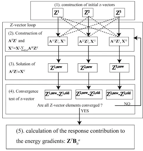
Equation(37), using definitions in Eqs.(34),(38),(40), and (41)gives the final formulation of the terms that are required to complete the FMO analytic gradient. The solution of these equations is accomplished as follows, illustrated in Fig. 1. By taking the I diagonal blocks of matrix A and solving
AI,ITZI =XI, one finds the initial ZI. XI is computed to solve Eq.(40). The external unknownsZK
kl in the last term of Eq.(39)are frozen, and this equation is decoupled for each fragmentI.Zis obtained by solving Eq.(40)for all fragments independently, and thenXI is updated with these new values ofZK for the next step; the calculations are then repeated until all elements in theZ-vector are self-consistent. This is simi-lar in both procedure and computational cost to the SCC pro-cedure in the monomer energy calculation (and it also bears a similarity to SCF), so it will be called the self-consistent Z-vector (SCZV) method. The preconditioned conjugate gra-dient method is applied to solve Eq. (40). The convergence test is made for allZ-vector elements. If the root-mean-square deviation ofZI,new−ZI,old is larger than a threshold, the pro-cedure returns to step 2 in Fig.1.
[image:8.612.312.558.49.310.2]The SCZV method is parallelized using the generalized distributed data interface (GDDI).89 Because of its iterative
FIG. 1. Schematic diagram of the SCZV procedure.
decoupled nature, the computation time of SCZV is compara-ble to that of SCC.
D. Application to the electrostatic dimer approximation
The previous subsection presented a derivation in which the analytic FMO gradient was derived with no approxima-tions. In this subsection, the electrostatic dimer (ES-DIM) ap-proximation for the fully analytic energy gradients is intro-duced, and it is shown that the response terms arising from the ES-DIM approximation need not be considered, because they cancel out with the response term from Eq.(19).
For separated fragmentsIandJ, if the distanceRI J (de-fined as the distance between the closest atoms inIandJ di-vided by the sum of their van der Waals atomic radii) is larger than the threshold valueLES−DIMin the ES-DIM
approxima-tion, the internal pair interaction energy, i.e., the correspond-ing summand in the second sum on the right-hand side of Eq. (1)can be replaced by
EI J −EI −EJ ≈Tr(DIuJ)+Tr(DJuI)
+
μν∈I
λσ∈J
DμνI DλσJ (μν|λσ)+ENRI J,
(42)
where the NR termENRI J =ENRI J −ENRI −ENRJ . In addition, the corresponding IJterm in the third sum of Eq. (1) can-cels out because DI J =0. The differentiation of Eq. (42) with respect to nuclear coordinatea without considering the response term is given elsewhere.83Therefore, it is sufficient
here to discuss how the unknown orbital response terms in the FMO gradient are formulated. The collection of the response
terms in the FMO gradient yields
Ua+ a = − N
I
Ua,I,I − N
I>J
Ua,I J,I J −Ua,I,I −Ua,J,J
+ N
I>J
Ua,I J,I J −Ua,I,I J −Ua,J,I J
+4 N
I>J
K=I J
μν∈I J vir
r∈K occ
i∈K
DμνI JUr ia,K(μν|r i).
(43)
As mentioned before,Ua =0 only if there are no approx-imations to the ESPs. In the case of the ES-DIM approxima-tion, Eq.(43)should be reformulated.
When the ES-DIM approximation is applied to avoid SCF calculations for dimers separated by more thanLES−DIM,
Uain Eq.(19)can be rewritten as
Ua = − N
I Ua,I,I
−
N
I>J(RI J≤LES−DIM)
Ua,I J,I J −Ua,I,I −Ua,J,J
+
N
I>J(RI J≤LES−DIM)
Ua,I J,I J −Ua,I,I J−Ua,J,I J
= − N
I
Ua,I,I +
N
I>J(RI J≤LES−DIM)
Ua,I,I(J)+Ua,J,J(I)
=0, (44)
where the partial terms
Ua,X,X(Y)=4
occ
i∈X vir
r∈X
Ur ia,Xur iY +vr iY, (45)
describe the contribution of a single fragment denotedYto the full sum over allYinUa,X,X.
Also, the following relation can be used:
Ua,I,I−Ua,I,I J =Ua,I,I(J), (46)
because [see Eq. (14)] the ESP for I J (VI J) runs over all fragments excludingIandJ, whereas the ESP forIexcludes the contribution from I. Therefore, in the difference expres-sion onlyJterms remain:
Vr iI −Vr iI J =Vr iI,I(J)≡ur iJ +vr iJ. (47)
Ua in Eq.(44)is in general nonzero and can be further simplified to
Ua = − N
I
Ua,I,I +
N
I>J(RI J≤LES−DIM)
Ua,I,I(J)+Ua,J,J(I)
= − N
I>J(RI J>LES−DIM)
Ua,I,I(J)+Ua,J,J(I), (48)
where the completeness relation is used:
N
I
Ua,I,I = N
I N
J=I
Ua,I,I(J)= N
I>J
Ua,I,I(J)+Ua,J,J(I).
(49)
For the derivatives of Eq.(42)the collection of response terms for allIJis
N
I>J(RI J>LES−DIM)
Tr
∂DI ∂a u
J
+Tr
∂DJ ∂a u
I + μν∈I λσ∈J ∂DμνI
∂a D J
λσ(μν|λσ)
+ μν∈I
λσ∈J
DμνI ∂D J λσ
∂a (μν|λσ)
=
N
I>J(RI J>LES−DIM)
Ua,I,I(J)+Ua,J,J(I)
−2
N
I=J(RI J>LES−DIM) occ
i j∈I
Saj i,IuJj i+vJj i. (50)
The first term on the right-hand side of Eq.(50)cancels out withUain Eq.(48). Since the derivative terms of Eq.(42) are already implemented,83 one can obtain the fully analytic
energy gradients for the ES-DIM approximation by calculat-ing the followcalculat-ing response contribution to the gradient:
Ua+ a
= 4
N
I>J(RI J≤LES−DIM)
K=I J
μν∈I J vir
r∈K occ
i∈K
DμνI JUr ia,K(μν|r i).
(51)
E. Implementation
To further facilitate solution of the SCZV equations, it is useful to reformulate them in the AO basis, thereby avoiding the expensive integral transformation.90 Examining
Eqs. (39), (32), and(33), the main computational effort is spent on two-electron integral terms like kl(kl|r i)Z
K kl in Eq.(39). By utilizing the MOi expansion over AOsμ,
|i = μ
Cμi|μ. (52)
The two-electron integral terms in Eq.(39)can be trans-formed according to
vir
k∈K occ
l∈K
(kl|r i)ZklK =
vir
k∈K occ
l∈K
CμKk∗CνKl(μν|r i)ZklK
= μν
(μν|r i) ˜ZμνK, (53)
124115-7 Fully analytic energy gradient in FMO J. Chem. Phys.134, 124115 (2011)
where
˜ ZμνK =
vir
k∈K occ
l∈K
CμKk∗ZklKCνKl. (54)
Using Eq. (53) avoids the full transformation of the two-electron integrals to the MO basis, which leads to a significant reduction of the computation time and memory. However, ˜ZμνI is not symmetric; this is inconvenient and can be further im-proved by symmetrizing it:
ZμνI =1 2
˜
ZμνI +Z˜νμI . (55)
It is possible to rewrite the SCZV equations [Eq. (40)] using the symmetrized localZ-vector elementZKμν.ZμνK cor-responds to the density matrix element Dμν in typical inte-gral programs, and therefore the SCZV method can be imple-mented using standard CPHF codes.
The Cauchy–Schwarz inequality, which estimates the value of (μν|ρσ) based on the values of a smaller set of integrals with repeated indices, can be used in the SCZV to obtain a further reduction of computation time. The Cauchy–Schwarz inequality screening is usually applied to
the maximum element of the factor by which the integrals of interest are multiplied. The SCZV procedure is more ef-ficient because theZ-vector elements normally have smaller values than the density matrix elements, and therefore, the Cauchy–Schwarz integral screening can skip more terms. In the implementation of the response contribution, Eq. (37), the direct (AO basis) algorithm and the Cauchy–Schwarz inequality for the calculation of the two-electron integrals are included. As a result, the calculations do not need a large amount of disk space or memory.
III. COMPUTATIONAL DETAILS
To verify that the response contribution that has been derived and implemented in this study makes the FMO en-ergy gradients fully analytic, analytic gradients are compared with numerical gradients for molecular systems taken from previous studies:80,91,92 (H
2O)64, the α-helix conformation
of the alanine decamer (ALA)10 capped with –OCH3 and
–NHCH3 groups, chignolin (PDB ID: 1UAO) solvated by
[image:10.612.61.553.332.722.2]157 water molecules, and the Trp-cage miniprotein construct (PDB ID: 1L2Y). The structures of (ALA)10 and 1L2Y were
FIG. 2. Geometric structures of (a) (H2O)64, (b) (ALA)10capped with CH3CO– and –NHCH3groups, (c) chignolin solvated by 157 water molecules, and (d)
1L2Y [colored by chemical elements as light grey (H), dark grey (C), blue (N), and red (O)].
taken from earlier works.83,92 Numerical gradients were computed with double differencing and a coordinate step of 0.005 Å [except for (H2O)64with 6–311G(d), where a 0.0005
Å step was used].
For the fragmentation of a system that does not require fragmenting covalent bonds, such as a water cluster, the HOP operator is not needed. For the first test calculation, a water molecule in (H2O)64is assigned to a fragment. The
geomet-rical structure of (H2O)64 was modeled byHYPERCHEM,
op-timized by AMBER94,93 and then reoptimized at the
FMO-RHF/6–31G level.80 The optimized structure of (H 2O)64 is
depicted in Fig.2(a).
For molecular systems in which fragmentation occurs across covalent bonds, the hybrid orbital operator contributes to the gradients both directly and via the response term from the Fock derivative, Eq. (25). The α-helix conformation of (ALA)10 with some intramolecular hydrogen bonds [shown
in Fig.2(b)] is chosen because in the case of incomplete ana-lytic gradients it is expected to have large errors in the gradi-ents compared to theβ-strand or extended structures. Because this system is relatively small, the validity of the analytic gra-dients without approximations can also be accessed.
The FMO method has been interfaced with the ef-fective fragment potential (EFP) method, which explicitly treats solvent molecules by adding a one-electron potential to the Hamiltonian.91,94 Chignolin is immersed in 157 water
molecules described by EFPs, and its structure is optimized using the combined FMO/EFP method at the RHF/cc-pVDZ level.91 The optimized structure in Fig. 2(c)reproduces the
PDB NMR structure well.80
Figure2(d)depicts the structure of 1L2Y. Because 1L2Y is the largest system treated with the FMO method in this study, it is an appropriate test case for the application of the electrostatic dimer approximation which is necessary for effi-cient computations of large systems. In this calculation, the threshold for the ES-DIM approximation LES−DIM was set to the default value, 2.0 and all other approximations were turned off.34
For systems fragmented across covalent bonds, i.e., (ALA)10, chignolin and 1L2Y, a one residue/one fragment
partition was adopted. The gradient calculations for (H2O)64,
(ALA)10, hydrated chignolin, and 1L2Y were performed at
the RHF/6–31G(d) level and diffuse functions were added to the carboxyl groups of 1L2Y. Additionally, RHF/6–311G(d) was also used to calculate the gradients for (H2O)64.
[image:11.612.53.296.677.750.2]The computation time of the SCZV procedure is ex-pected to be comparable to that of the SCC calculation. Thus, the timings of the calculations of fully analytic gradients in which both the SCC and SCZV steps were included were measured and compared. The timing calculations used the 32
TABLE I. The number of GDDI groups used in dividing 31 nodes.
Monomer step Dimer step
(H2O)64 16 16
(ALA)10 5 15
Hydrated chignolin 5 15
1L2Y 10 15
nodeSOROBANcluster with Intel Pentium 4 central process-ing unit (CPU) 3.2 GHz nodes connected by Gigabit Ethernet. TableIlists separately for monomers and dimers the number of GDDI groups in the gradient calculation for each system (in GDDI, in order to improve parallel efficiency, all computer nodes are divided into groups and individual monomer and dimer calculations are distributed dynamically among these groups). Note that the number of GDDI groups in the SCZV step is the same as in the SCC step. The parallel efficiency is calculated for the gradient and SCZV calculations for (H2O)64
using 1, 2, 4, 8, 16, and 32 nodes of theSOROBANcluster. For this calculation, the number of GDDI groups is equal to the number of nodes.
IV. RESULTS AND DISCUSSION
A. Fully analytic energy gradients without approximations
In this subsection, the fully analytic gradients without approximations are discussed. It is important to numerically verify that the gradients are fully analytic using Ua=0 [Eq.(19)].
As mentioned previously, for (H2O)64, the energy
gradi-ents do not involve the HOP term and only the response term contributes to the analytic gradients. In Table II, the root-mean-square (RMS) value in the numerical gradients became identical with the new analytic gradients (0.005997 a.u.). However, the RMS value in the old (conventional) analytic gradients, in which only the response contribution is ne-glected, deviates by 0.0001 a.u. from the numerical and the analytic ones. For the maximum absolute gradient values (MAX grad.), the new analytic gradient value is in good agreement with the corresponding numerical value, while the conventional value differs by 0.00025 a.u. The latter is not a negligible error when aiming for fully analytic gradients. The RMS of the errors for the new analytic gradient relative to the numerical gradient (the RMS error in the analytic gradients) is negligibly small (0.000011 a.u.), which is an improvement by a factor of 20 over the RMS error in the old analytic gradients (0.000231 a.u.). This improvement is visualized in Fig. 3(a), which plots the errors of the new analytic gradient and the old analytic gradient relative to the numeric gradient against the total 576 gradient elements. The new analytic gradient values converge to zero, while the old analytic gradient values have large deviations.
For systems fragmented across covalent bonds, the HOP contribution to the response term must be considered. (ALA)10is such a system and due to its size is a good test for
calculating numerical gradients without approximations at a relatively moderate computational cost. Note that the old an-alytic gradient method that is illustrated here did include the direct contribution of HOP derivatives to the gradients, since this contribution was introduced in a previous study.84TableII shows that the three types of gradients are in good agreement. Even though the RMS value in the old analytic gradients is very close to that of numerical gradients, the RMS errors and maximum absolute gradient error for the old analytic gradient deviates by significant amounts (0.000160 and 0.000580 a.u., respectively). On the other hand, the very small errors
124115-9 Fully analytic energy gradient in FMO J. Chem. Phys.134, 124115 (2011)
TABLE II. The RMS and the maximum absolute values (MAX grad.) of the gradient elements for FMO2–RHF. RMS of the errors of the analytic gradients relative to the numeric gradients (RMS error) and the error in the maximum absolute gradient values (MAX error). All values are in a.u.
Gradient RMS MAX grad. RMS error MAX error
(H2O)64without approximations, 6–31G(d)
Numeric 0.005997 0.014090 . . . .
Analytic 0.005997 0.014094 0.000011 0.000035
Conventional 0.006132 0.014347 0.000231 0.000961
(H2O)64withLES−DIM=2.0, 6–31G(d)
Numeric 0.005997 0.014090 . . . .
Analytic 0.005997 0.014094 0.000011 0.000034
Conventional 0.006132 0.014347 0.000232 0.000975
(H2O)64withLES−DIM=2.0, 6–311G(d)
Numeric 0.007467 0.018020 . . . .
Analytic 0.007469 0.018029 0.000003 0.000010
Conventional 0.007745 0.018507 0.000433 0.002280
(ALA)10without approximations, 6–31G(d)
Numeric 0.011658 0.043197 . . . .
Analytic 0.011664 0.043222 0.000009 0.000039
Conventional 0.011655 0.043169 0.000160 0.000580
Hydrated (EFP) chignolin without approximations, 6–31G(d)
Numeric 0.000284 0.002010 . . .
Fully analytic 0.000280 0.001995 0.000017 0.000092
Conventional 0.000215 0.001542 0.000191 0.001501
1L2Y withLES−DIM=2.0, 6–31G(d)
Numeric 0.019779 0.047540 . . . .
Analytic 0.019780 0.047543 0.000015 0.000037
Conventional 0.019822 0.047418 0.000335 0.001001
in the new analytic gradient values indicate that they are fully analytic, and that the HOP contribution to the response term is properly included. In Fig. 3(b), as in Fig. 3(a), one can see that the new analytic gradients are fully analytic for every gradient element. Comparing Fig.3(b)((ALA)10) with
Fig.3(a)(the water cluster), the former has smaller gradient errors for the old analytic gradients. Since the response term is related to the ESPs, the environmental potential affects the water clusters more significantly than the polypeptide.
Most biological processes occur in aqueous solution. To model one of these processes, one may consider a protein in a water droplet. For molecular dynamics and geometry opti-mization processes, an accurate solvent model must be com-bined with the application of FMO to the solute. As the first test calculation toward this goal, hydrated chignolin is chosen for the FMO/EFP framework. In order to obtain the fully ana-lytic energy gradients in this framework, it is necessary to add the EFP derivatives to the Fock derivative term, Eq.(25)and probably to modify the Amatrix in Eq.(38). In this study, however, the EFP-related many-body polarization contribu-tion to the FMO ESP response term was neglected. There-fore, the FMO/EFP energy gradients are not fully analytic. So, the accuracy of the FMO/EFP new energy gradients is shown only for the solute (FMO) molecule (chignolin). As seen in TableII, the accuracy of the FMO/EFP new energy gradients is similar to that for the full treatment of FMO, but the max-imum absolute gradient error is larger (0.000092 a.u.) than those for the other test systems, and there are slight deviations
in the FMO/EFP new analytic gradients in Fig.3(c). Never-theless, the maximum absolute new analytic gradient error is improved by a factor of 16 compared to the old analytic gradi-ent value. This encouraging result provides motivation to de-velop the fully analytic energy gradients for FMO/EFP as well as FMO combined with the polarizable continuum model.92,95
For the chosen systems, the wall clock times required for the SCC, the SCZV, and the total FMO calculation were measured. Table III shows that for the gradient calculation without approximations for (H2O)64, the SCC calculation
took 24.3 s, which is comparable to 29.5 s. in the correspond-ing SCZV calculation. These times are small relative to the total computational time of over 400 s. For (ALA)10, the
SCZV calculation takes only 64% of the computation time of the corresponding SCC calculation. For hydrated chignolin, the SCZV calculation requires a similar percentage of the computation time. These results illustrate why theZ-vectors converge more rapidly; the calculation of two-electron integrals is faster because the Cauchy–Schwarz inequality is more efficient when applied to the Z-vectors rather than to the monomer densities (used in ESPs or two-electron integrals for monomers).
B. Fully analytic energy gradients in the ES dimer approximation
The FMO energy gradients have been shown to be fully analytic by introducing the response contribution. The putation time in the calculation of the response term is
FIG. 3. Errors of the analytic gradient elements relative to the numeric gradient elements for (a) (H2O)64, (b) (ALA)10capped with CH3O– and –NHCH3
groups, (c) chignolin solvated by 157 water molecules, (d) 1L2Y, all calculated at the RHF/6–31G(d) level, and (e) (H2O)64at the RHF/6–311G(d) [all the
gradient elements for (a)–(c), (e), and the representative elements for (d)]. Black diamond: fully analytic energy gradients. Yellow square: the conventional gradients.
parable to or less than that required for the SCC calculation. This implies that although it is practical to calculate the re-sponse term itself, it is still expensive to calculate the fully analytic energy gradients for a larger molecule because of the difficulty in performing a large number of dimer SCF calcu-lations without approximations.
As discussed above, the fully analytic energy gradients with the ES-DIM approximation have been derived. The
pur-pose of this subsection is to check numerically that the FMO energy gradients are fully analytic within the ES-DIM approx-imation and to discuss the timings.
The ES-DIM approximation was first applied to (H2O)64
using both the 6–31G(d) and 6–311(d) basis sets. Table II shows that withLES−DIM=2.0, the RMS value, the MAX gra-dient value, and the RMS error for the new analytic gragra-dients are identical to those without approximations. Additionally,
124115-11 Fully analytic energy gradient in FMO J. Chem. Phys.134, 124115 (2011)
TABLE III. Wall clock time in the SCC, SCZV, and the total computa-tion using a 31 single 3.2 GHz Pentium 4 cluster (all in seconds), FMO2-RHF/6–31G(d).
SCC SCZV TOTAL
(H2O)64without approximations
Analytic 24.3 29.5 467.2
Conventional 23.0 . . . 431.4
(H2O)64withLES−DIM=2.0
Analytic 29.4 28.1 261.0
Conventional 24.3 . . . 227.8
(ALA)10without approximations
Analytic 359.7 230.4 1240.3
Conventional 358.4 . . . 1016.3
hydrated chignolin without approximations
Analytic 1383.6 883.2 7299.8
Conventional 1382.4 . . . 6419.2
1L2Y withLES−DIM=2.0
Analytic 3429.1 2320.7 12942.1
Conventional 3380.4 . . . 10597.1
the maximum gradient error is negligibly small. These results imply that the ES-DIM approximation is a suitable choice for this system.
The errors for the old analytic gradient increase with the basis set, as can be seen in Table II. For example, the maximum gradient error increases from 0.000975 to 0.002280 when going from 6–31G(d) to 6–311(d). The error in the new analytic versus numeric gradient is about 15 times smaller and is probably due to the error in the numerical gradient itself. There is also no basis set effect on the error when the new analytic gradient is employed. The pictorial representations of the errors in Figs. 3(a)and 3(e) demonstrate the quality of the gradients.
For another system requiring fragmentation across cova-lent bonds, consider 1L2Y, which consists of 20 amino acid residues. Since the calculation of numerical gradients for such a relatively large molecule is time consuming, a subsystem is chosen, i.e., the 38 atoms defining 19 detached bonds be-tween 20 fragments (for which atoms the error in the old an-alytic gradient is the largest as found in the earlier study84).
With LES−DIM=2.0, there are 92 SCF and 98 approximated (ES-DIM) dimers. In Table II[see also Fig. 3(d)], the cor-responding RMS value and the maximum absolute gradient value show that the new analytic gradients are fully analytic in comparison to the numerical values. The corresponding RMS and MAX gradient errors are similar in accuracy to the fully analytic gradient values of the other systems. The errors are much improved compared to those from the old analytic gra-dient calculation, especially for the MAX gragra-dient which is more accurate by a factor of 27, indicating a significant con-tribution from the response term in this system.
As shown in TableIII, for (H2O)64, the total wall clock
[image:14.612.55.295.81.295.2]time for the fully analytic gradient calculation with the ap-proximation (261.0 s) is less than the timing without approx-imations (467.2 s). In comparing the SCZV and the SCC cal-culation for this water cluster, it is reasonable that the former took less computation time. When using the approximation,
FIG. 4. The parallel efficiency using the personal computer cluster of 1, 2, 4, 8, 16 and, 32 CPUs (Intel Pentium 4 3.2 GHz). Solid line: for the total gradient calculation. Dashed line: for the SCZV calculation.
the ratio of the computation time in SCZV to SCC is normally less than 1. This implies that the SCZV calculation is faster; this trend is independent of the ES-DIM approximation. For 1L2Y, the SCZV calculations took approximately 70% of the time required for the SCC calculations, and it is expected that this ratio will decrease for larger systems.
For (H2O)64, the parallel efficiencyS(n), shown in Fig.4,
was calculated using the following expression:
S(n)= T1 Tn
n ×100, (56)
where T1 and Tn represent the computation time using 1 node and n nodes, respectively. Hundred percent efficiency means that the calculation isn times faster onn nodes. The results show that for (H2O)64 the parallel efficiency is over
97.8% for all numbers of nodes (n=1, 2, 4, 8, 16, and 32) both in the total gradient calculation (solid line) and SCZV calculation (dashed line). Forn =16, the parallel efficiency in the SCZV calculation drops slightly from that forn =8. For (H2O)64, 64 SCZV calculations should be distributed
into 16 nodes (divided into 16 GDDI groups). However, each SCZV calculation takes a different amount of time, because the number of iterations and the integral screening depend upon the fragment; the GDDI calculations are dynamically divided over groups, and there is some granularity (i.e., some groups finish ahead of others). This is why the parallel efficiency drops atn=16. The superlinear scaling over 100% for a small number of nodes is also observed in FMO–RHF calculations89 and is thought to originate from external factors like CPU cache efficiency.
V. CONCLUSIONS
The CPHF equations and the Z-vector equations in the FMO framework have been derived to compute the fully an-alytic energy gradients. One outcome of this study is the derivation and implementation of the SCZV equations, by which the time-consuming Z-vector equations of the whole system reduce to those of the monomer fragments. Addi-tionally, the SCZV procedure is parallelized by the use of
GDDI.89 It was shown that the FMO energy gradients are fully analytic in the electrostatic dimer approximation. This leads to a significant reduction of the total computation time. Nearly fully analytic energy gradients have been successfully implemented for the combined FMO/EFP method as well.
The use of the SCZV procedure is not limited to the gradient calculation. The calculation of the second derivative (Hessian) matrix is necessary to calculate important prop-erties such as the IR spectrum, Raman spectrum, and NMR chemical shifts. To calculate the fully analytic Hessian, one must solve the CPHF equations, and the SCZV procedure would play an essential role. The SCZV procedure could also be found useful in other fragmentation methods that require the response term (some methods87,96 do not need it with
respect to the field, although the Mulliken charge derivatives do require it97,80).
The analytic gradient equations have been derived at the Hartree–Fock level of theory. For proteins, dispersion is crucial for determining the folded structure58 and for protein-ligand binding. Therefore, the fully analytic energy gradient should be extended to electron correlation methods such as MP2. For practical calculations, such as FMO–MD to study protein folding, it will be necessary to develop the fully analytic gradient with the point charge (ESP–PTC) approximation.
As mentioned earlier, MD simulations are an important application of FMO; however, FMO–MD has been limited mainly to molecular clusters.70–72,75–78As found in this study,
with the introduction of fully analytic energy gradients, re-liable MD simulation with perfect energy conservation will now be possible.
ACKNOWLEDGMENTS
This work has been supported by the Next Generation Super Computing Project, Nanoscience Program (MEXT, Japan), and by a US National Science Foundation Petascale Applications grant. K.B. is supported by a US Department of Energy Computational Science Graduate Fellowship.
1D. A. Pearlman, D. A. Case, J. W. Caldwell, W. S. Ross, T. E. Cheatham,
S. Debolt, D. Ferguson, G. Seibel, and P. Kollman, Comput. Phys. Commun.91, 1 (1995).
2P. Kollman, I. Massova, C. Reyes, B. Kuhn, S. H. Huo, L. Chong, M. Lee,
T. Lee, Y. Duan, W. Wang, O. Donini, P. Cieplak, J. Srinivasan, D. A. Case, and T. E. Cheatham,Acc. Chem. Res.33, 889 (2000).
3D. Bashford and D. A. Case,Annu. Rev. Phys. Chem.51, 129 (2000). 4J. Gao and D. Truhlar,Annu. Rev. Phys. Chem.53, 467 (2002). 5A. D. Mackerell,J. Comput. Chem.25, 1584 (2004).
6W. Wang, O. Donini, C. M. Reyes, and P. A. Kollman,Annu. Rev. Biophys. Biomol. Struct.30, 211 (2001).
7A. Warshel,Annu. Rev. Biophys. Biomol. Struct.32, 425 (2003). 8R. Car and M. Parrinello,Phys. Rev. Lett.55, 2471 (1985). 9J. L. Gao,J. Phys. Chem. B101, 657 (1997).
10J. L. Gao,J. Chem. Phys.109, 2346 (1998).
11H. B. Schlegel, J. M. Millam, S. S. Iyengar, G. A. Voth, A. D. Daniels, G.
E. Scuseria, and M. J. Frisch,J. Chem. Phys.114, 9758 (2001).
12W. Xie and J. Gao,J. Chem. Theory Comput.3, 1890 (2007).
13W. Xie, M. Orozco, D. G. Truhlar, and J. Gao,J. Chem. Theory Comput. 5, 459 (2009).
14S. Y. Wu and C. S. Jayanthi,Phys. Rep.358, 1 (2002).
15S. Goedecker and G. E. Scuseria,Comput. Sci. Eng.5, 14 (2003).
16D. Hankins, J. W. Moskowitz, and F. H. Stillinger,J. Chem. Phys.53, 4544
(1970).
17K. Morokuma,J. Chem. Phys.55, 1236 (1971).
18K. Ohno and H. Inokuchi,Theor. Chim. Acta26, 331 (1972). 19P. Otto and J. Ladik,Chem. Phys.8, 192 (1975).
20H. Stoll and H. Preuß,Theor. Chim. Acta46, 11 (1977). 21Z. Barandiaran and L. Seijo,J. Chem. Phys.89, 5739 (1988).
22H. Kubota, Y. Aoki, and A. Imamura, Bull. Chem. Soc. Jpn 67, 13
(1994).
23H. R. Leverentz and D. G. Truhlar, J. Chem. Theory Comput.5, 1573
(2009).
24M. S. Gordon, J. M. Mullin, S. R. Pruitt, L. B. Roskop, L. V. Slipchenko,
and J. A. Boatz,J. Phys. Chem. B113, 9646 (2009).
25R. A. Mata, H. Stoll, and B. J. C. Cabral,J. Chem. Theory Comput.5, 1829
(2009).
26L. Huang, L. Massa, I. Karle, and J. Karle,Proc. Natl. Acad. Sci. U.S.A. 106, 3664 (2009).
27Y. Tong, Y. Mei, J. Z. H. Zhang, L. L. Duan, and Q. G. Zhang,J. Theor. Comput. Chem.8, 1265 (2009).
28P. Söderhjelm and U. Ryde,J. Phys. Chem. A113, 617 (2009). 29S. D. Yeole and S. Gadre,J. Chem. Phys.132, 094102 (2010).
30A. Pomogaeva, F. L. Gu, A. Imamura, and Y. Aoki,Theor. Chem. Acc.125,
453 (2010).
31T. Touma, M. Kobayashi, and H. Nakai, Chem. Phys. Lett. 485, 247
(2010).
32X. He and K. M. Merz,J. Chem. Theory Comput.6, 405 (2010). 33K. Kitaura, E. Ikeo, T. Asada, T. Nakano, and M. Uebayasi,Chem. Phys.
Lett.313, 701 (1999).
34T. Nakano, T. Kaminuma, T. Sato, K. Fukuzawa, Y. Akiyama, M. Uebayasi,
and K. Kitaura,Chem. Phys. Lett.351, 475 (2002).
35D. G. Fedorov and K. Kitaura,J. Phys. Chem. A111, 6904 (2007). 36The Fragment Molecular Orbital Method: Practical Applications to Large
Molecular Systems, edited by D. G. Fedorov and K. Kitaura (CRC Press, Boca Raton, FL, 2009).
37D. G. Fedorov and K. Kitaura,Chem. Phys. Lett.433, 182 (2006). 38J. L. Pascual and L. Seijo,J. Chem. Phys.102, 5368 (1995).
39Q. Cui, M. Elstner, E. Kaxiras, T. Frauenheim, and M. Karplus,J. Phys. Chem. B105, 569 (2001).
40D. G. Fedorov and K. Kitaura,J. Chem. Phys.121, 2483 (2004). 41Y. Mochizuki, K. Yamashita, K. Fukuzawa, K. Takematsu, H. Watanabe, N.
Taguchi, Y. Okiyama, M. Tsuboi, T. Nakano, and S. Tanaka,Chem. Phys. Lett.493, 346 (2010).
42D. G. Fedorov and K. Kitaura,J. Chem. Phys.123, 134103/1 (2005). 43S.-I. Sugiki, N. Kurita, Y. Sengoku, and H. Sekino,Chem. Phys. Lett.382,
611 (2003).
44D. G. Fedorov and K. Kitaura,Chem. Phys. Lett.389, 129 (2004). 45D. G. Fedorov and K. Kitaura,J. Chem. Phys.122, 054108/1 (2005). 46Y. Mochizuki, S. Koikegami, S. Amari, K. Segawa, K. Kitaura, and T.
Nakano,Chem. Phys. Lett.406, 283 (2005).
47Y. Mochizuki, K. Tanaka, K. Yamashita, T. Ishikawa, T. Nakano, S. Amari,
K. Segawa, T. Murase, H. Tokiwa, and M. Sakurai,Theor. Chem. Acc.117, 541 (2007).
48M. Chiba, D. G. Fedorov, and K. Kitaura,Chem. Phys. Lett.444, 346
(2007).
49M. Chiba, D. G. Fedorov, and K. Kitaura,J. Chem. Phys.127, 104108
(2007).
50M. Chiba, D. G. Fedorov, and K. Kitaura,J. Comput. Chem.29, 2667
(2008).
51S. R. Pruitt, D. G. Fedorov, K. Kitaura, and M. S. Gordon,J. Chem. Theory Comput.6, 1 (2010).
52B. Auer, M. V. Pak, and S. Hammes-Schiffer,J. Phys. Chem. C114, 5582
(2010).
53I. Nakanishi, D. G. Fedorov, and K. Kitaura,Proteins: Struct., Funct., Bioinf.68, 145 (2007).
54T. Sawada, T. Hashimoto, H. Tokiwa, T. Suzuki, H. Nakano, H. Ishida, M.
Kiso, and Y. Suzuki,Glycoconjugate J.25, 805 (2008).
55T. Watanabe, Y. Inadomi, K. Fukuzawa, T. Nakano, S. Tanaka, L. Nilsson,
and U. Nagashima,J. Phys. Chem. B111, 9621 (2007).
56T. Sawada, D. G. Fedorov, and K. Kitaura,Int. J. Quantum Chem.109,
2033 (2009).
57T. Ishida, D. G. Fedorov, and K. Kitaura,J. Phys. Chem. B110, 1457
(2006).
58X. He, L. Fusti-Molnar, G. Cui, and K. M. J. Merz,J. Phys. Chem. B113,
5290 (2009).
![FIG. 2. Geometric structures of (a) (H2O)64, (b) (ALA)10 capped with CH3CO– and –NHCH3 groups, (c) chignolin solvated by 157 water molecules, and (d)1L2Y [colored by chemical elements as light grey (H), dark grey (C), blue (N), and red (O)].](https://thumb-us.123doks.com/thumbv2/123dok_us/8127261.241281/10.612.61.553.332.722/geometric-structures-chignolin-solvated-molecules-colored-chemical-elements.webp)


